Silly String Derivation of the Wave Equation

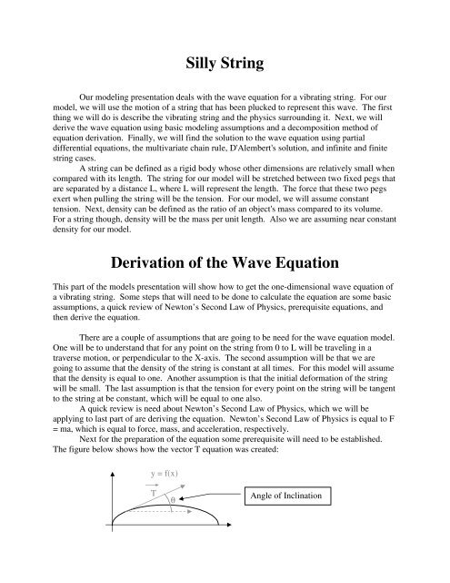
Silly StringOur modeling presentation deals with the wave equation for a vibrating string. For ourmodel, we will use the motion of a string that has been plucked to represent this wave. The firstthing we will do is describe the vibrating string and the physics surrounding it. Next, we willderive the wave equation using basic modeling assumptions and a decomposition method ofequation derivation. Finally, we will find the solution to the wave equation using partialdifferential equations, the multivariate chain rule, D'Alembert's solution, and infinite and finitestring cases.A string can be defined as a rigid body whose other dimensions are relatively small whencompared with its length. The string for our model will be stretched between two fixed pegs thatare separated by a distance L, where L will represent the length. The force that these two pegsexert when pulling the string will be the tension. For our model, we will assume constanttension. Next, density can be defined as the ratio of an object's mass compared to its volume.For a string though, density will be the mass per unit length. Also we are assuming near constantdensity for our model.Derivation of the Wave EquationThis part of the models presentation will show how to get the one-dimensional wave equation ofa vibrating string. Some steps that will need to be done to calculate the equation are some basicassumptions, a quick review of Newton’s Second Law of Physics, prerequisite equations, andthen derive the equation.There are a couple of assumptions that are going to be need for the wave equation model.One will be to understand that for any point on the string from 0 to L will be traveling in atraverse motion, or perpendicular to the X-axis. The second assumption will be that we aregoing to assume that the density of the string is constant at all times. For this model will assumethat the density is equal to one. Another assumption is that the initial deformation of the stringwill be small. The last assumption is that the tension for every point on the string will be tangentto the string at be constant, which will be equal to one also.A quick review is need about Newton’s Second Law of Physics, which we will beapplying to last part of are deriving the equation. Newton’s Second Law of Physics is equal to F= ma, which is equal to force, mass, and acceleration, respectively.Next for the preparation of the equation some prerequisite will need to be established.The figure below shows how the vector T equation was created:y = f(x)TθAngle of Inclination

T= 1+1dydx2i+1+dydxdydx2jTNext a small chunk of the string is needed to calculate the one-dimensional wave equation. Asshow in the diagram below:Horizontal∆SForcesVerticalForcesSince all points on the string are going in a vertical motion the horizontal force of the vector Tcan be dropped. Hence, from all the information calculated so far the following equation can beestablished:T ∂u∂x ∂u1+ ∂x( x + ∆x,t)( x + ∆x,t)2−∂u∂x ∂u1+ ∂x( x,t)2((x,t) ∂u∂uAlso since the initial deformation of the string was small the ( x + ∆x,t)and the ((x,t)will∂x∂xget small, and since there squared they will go to zero faster. Plus, the tension T and the densityρ is equal to one, they can be dropped by the equation. This will then give us the equation:∂u∂x∂u∂x( x + ∆xt) − ( x,t) = ∆s( x,t)∂,22∂tuNet forcemassacceleration

Hence Newton’s Second Law of Physics is show here. The last thing that is needed to be doneis divide both sides by ∆x, which will then equal the one-dimensional wave equation:∂2∂xu2( )∂ ux, t = ( x,t)∂t22Derivation of two-dimensional wave equationThe next part of our modeling is coming up with the basis for our two-dimensional waveequation. The model is based on a second order homogeneous partial differential equation in theform of:222∂ y ∂ y ∂ y ∂y∂yA + B + C + D + E + Fy = 022∂x∂x∂y∂t∂x∂tThere are three different classifications of partial differential equations. Using the equationabove if ∆ = B*B – AC, and ∆>0 the equation is Hyperbolic, If ∆

That gives:F = f +2 2( u,v)= uv uLooking at a Variable Dependency Diagram you will see that:∂F∂f∂g∂f∂u= +∂x∂u∂x∂v∂xWhich is equal tox(( v 2 + 2u)(y cos( x))+ (2uv)eWith substitution this is broken down tox 2x x( e ) + 2ysin( x)(y cos( x))+ 2( y sin( x)e eThat shows the multivariable chain rule for the first derivative. The multivariable chain rule forthe second derivative is very close to that so we will use the same explanation to show it.The partial differential equation that we are going to work with is set up in the following matter:ξ = x – t and η = x + tSo therefore ξ + η = 2x and η - ξ = 2tNow using the Multi-Variable Chain Rule which we just established we have∂u∂u∂u= − +∂t∂ξ ∂ηSo therefore the partial of that is equal to2∂ u ∂ ∂u∂u= [ − + ]2∂t∂t∂ξ ∂ηUsing algebra to simplify this you get2∂ u2∂t=2∂ u2∂ξ2∂ u− 2 =∂η∂ξ2∂ u2∂ηAnd now with respect to x∂u∂u∂u= − +∂x∂ξ ∂ηSo therefore the partial of this equation is equal to2∂ u ∂ ∂u∂u= [ − + ]2∂t∂t∂ξ ∂ηUsing algebra to simplify this equation you get2∂ u2∂x=2∂ u2∂ξ2∂ u+ 2 =∂η∂ξ2∂ u2∂η

Now if you substitute2 2∂ u ∂ u=2 2∂x∂tYou end up getting that2∂ u4 = 0∂η∂ξSo we finally come up with2∂ u= 0∂η∂ξWhen ξ = x - t and η = x + tD’Alambert’s SolutionD’Alambart’s solution is a general solution to the one-dimensional wave equation found earlier.In order to find D’Alambert’s solution, two substitutions that we will be making will be thatη = x + tξ = x – tIn order to find D’Alambert’s solution we need to find the second partial of U with respect totime and second partial of U with respect to x, which were also found earlier. Substituting thesecond partial of U with respect to time and x back into the one-dimension wave equation gives22 2∂ u ∂ u ∂ u− 2 +22∂ε∂ndε∂n22 2∂ u ∂ u ∂ u= + 2 +22∂ε∂ndε∂nCanceling like terms and simplifying gives2∂ u= 0∂η∂εIf we integrate with respect to Ada, we get the partial of U with respect to Xi.∂u = k (ε )∂εIf we integrate then with respect to Xi, and simplify, we getu ( ε,η)= k(ε ) + c(η)

Relabeling in more conventional terms givesu ( ε,η)= f ( η)+ g(ε)Then substituting gives us D’Alambart’s Solution.u( x,t)= f ( x + t)+ g(x − t)Infinite String ProblemNext, we will find a solution to the infinite string problem. First we set some reasonable initialconditions.∂u( x,0)= 0∂tu( x,0)= φ(x)Next find the partial of U with respect to time∂u∂tand,=f '(x + t)− g'( x − t)∂u( x,0)= f '( x)− g'( x)∂tso,∂u( x,0)= f '( x)− g'( x)= 0∂tand also,u( x,t)= f ( x + t)+ g(x − t)remembering initial conditionsu( x,0)= f ( x)+ g(x)= φ(x)which gives us

f ( x)+ g(x)= φ(x)Now using the previous two equations, we have to solve for f and g. When we do solve for f andg, we get,c +φ(x)f ( x)=( x2) − cg(x)2= φ 2Now to find the solution to the Infinite String Problem, we need to plug f and g back into U, weget,φ(x + t)+ φ(x − t)U ( x,t)=Which is the solution to the Infinite String Problem.Infinite String ProblemNext we will find a solution to the finite string problem. In this example we will consider astring with endpoints 0 and L. For the finite string problem we will start out with the two initialconditions from the infinite string problem plus two others.u( x,0)= φ(x)∂u( x,0)= 0∂tu( 0, t)= 0u( L,t)= 0Using the solution to the infinite string problem, we can considerφ(t)+ φ(−t)u( 0, t)== 02φ(L + t)+ φ(L − t)u( L,t)== 02Now we can simplify these two equations by multiplying each side by two. Now take theequation u (0,t) and let b stand for t. Now through manipulation, we get the equationφ(b)= −φ( −b)

Then substitute L-t back in for b and come up with this equation.φ( L − t)= −φ( t − L)Which equalsφ( L + t)−φ(t − L)= 0Manipulating this equation gives usφ(x + 2L)−φ(x)= 0Which is the solution to the finite string problem. Now this is a periodic function with a periodof 2L. Because this function is periodic, it is often modeled using a series of sine and cosine's,which is more commonly known as the Fourier series.

Silly StringBy: Michael JanssenJeffery RogersNathaniel SmithZebulon ZielieMay 17, 2000

References:S.L. Sobolev. Partial Differential Equations of Mathematical Physics.Steve Deckelman. Math Models II Professor