Forecasting with ARIMA models

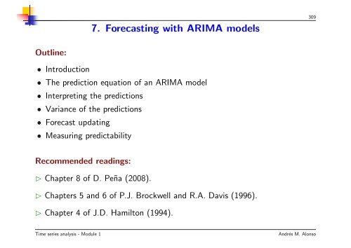
7. Forecasting with ARIMA models309Outline:• Introduction• The prediction equation of an ARIMA model• Interpreting the predictions• Variance of the predictions• Forecast updating• Measuring predictabilityRecommended readings:⊲ Chapter 8 of D. Peña (2008).⊲ Chapters 5 and 6 of P.J. Brockwell and R.A. Davis (1996).⊲ Chapter 4 of J.D. Hamilton (1994).Time series analysis - Module 1Andrés M. Alonso

Introduction310⊲ We will look at forecasting using a known ARIMA model. We will define theoptimal predictors as those that minimize the mean square prediction errors.⊲ We will see that the prediction function of an ARIMA model has a simplestructure:• The non-stationary operators, that is, if the differences and the constantexist they determine the long-term prediction.• The stationary operators, AR and MA, determine short-term predictions.⊲ Predictions are of little use without a measurement of their accuracy, andwe will see how to obtain the distribution of the prediction errors and how tocalculate prediction confidence intervals.⊲ Finally we will study how to revise the predictions when we receive newinformation.Time series analysis - Module 1

The prediction equation of an ARIMA model311Conditional expectation as an optimal predictor⊲ Suppose we have observed a realization of length T in a time seriesz T = (z 1 , ..., z T ), and we wish to forecast a future value k > 0 periods ahead,z T +k .⊲ We let ẑ T (k) be a predictor of z T +k obtained as a function of the T valuesobserved, that is, with the forecast origin in T , and the forecast horizon at k.⊲ Specifically, we will study linear predictors, which are those constructed asa linear combination of the available data:ẑ T (k) = α 1 z T + α 2 z T −1 + ... + α T z 1 .⊲ The predictor is well defined when the constants α 1 , ..., α T used to constructit are known.Time series analysis - Module 1

Conditional expectation as an optimal predictor312⊲ We denote by e T (k) the prediction error of this predictor, given by:e T (k) = z T +k − ẑ T (k)and we want this error to be as small as possible.⊲ Since the variable z T +k is unknown, it is impossible to know a priori theerror that we will have when we predict it.⊲ Nevertheless, if we know its probability distribution, that is, its possible valuesand probabilities, with a defined predictor we can calculate the probability ofits error being among the given values.⊲ To compare predictors we specify the desired objective by means of acriterion and select the best predictor according to this criterion.Time series analysis - Module 1

Conditional expectation as an optimal predictor313⊲ If the objective is to obtain small prediction errors and it does not matter ifthey are positive or negative we can eliminate the error sign using the criterionof minimizing the expected value of a symmetric loss function of the error,such as:l(e T +k ) = ce 2 T (k) or l(e T (k)) = c |e T (k)| ,where c is a constant.⊲ Nevertheless, if we prefer the errors in one direction,, we minimize theaverage value of an asymmetric loss function of the error which takes intoaccount our objectives. For example,l(e T (k)) ={c1 |e T (k)| , if e T (k) ≥ 0c 2 |e T (k)| , if e T (k) ≤ 0}(130)for certain positive c 1 and c 2 . In this case, the higher the c 2 /c 1 ratio the morewe penalize low errors.Time series analysis - Module 1

314Example 66. The figure compares the three above mentioned loss functions.The two symmetric functionsl 1 (e T (k)) = e 2 T (k), y l 2 (e T (k)) = 2 |e T (k)| ,and the asymmetric (130) have been represented using c 1 = 2/3 and c 2 = 9/2.12108642l 1(symmetric)l 2(symmetric)l 3(asymmetric)0-3 -2 -1 0 1 2 3⊲ Comparing the two symmetricfunctions, we see that thequadratic one places lessimportance on small values thanthe absolute value function,whereas it penalizes large errorsmore.⊲ The asymmetric function giveslittle weight to positive errors,but penalizes negative errorsmore.Time series analysis - Module 1

Conditional expectation as an optimal predictor315⊲ The most frequently utilized loss function is the quadratic, which leads tothe criterion of minimizing the mean square prediction error (MSPE) of z T +kgiven the information z T . We have to minimize:MSP E(z T +k |z T ) = E [ (z T +k − ẑ T (k)) 2 |z T]= E[e2T (k)|z T]where the expectation is taken with respect to the distribution of the variablez T +k conditional on the observed values z T .⊲ We are going to show that the predictor that minimizes this mean squareerror is the expectation of the variable z T +k conditional on the availableinformation.⊲ Therefore, if we can calculate this expectation we obtain the optimalpredictor without needing to know the complete conditional distribution.Time series analysis - Module 1

Conditional expectation as an optimal predictor316⊲ To show this, we letµ T +k|T = E [z T +k |z T ]be the mean of this conditional distribution. Subtracting and adding µ T +k|Tin the expression of MSP E(z T +k ) expanding the square we have:MSP E(z T +k |z T ) = E [ (z T +k − µ T +k|T ) 2 |z T]+ E[(µT +k|T − ẑ T (k)) 2 |z T]since the double product is cancelled out.(131)⊲ Indeed, the term µ T +k|T − ẑ T (k) is a constant, since ẑ T (k) is a function ofthe past values and we are conditioning on them and:thus we obtain (131).E [ (µ T +k|T − ẑ T (k))(z T +k − µ T +k|T )|z T]== (µ T +k|T − ẑ T (k))E [ (z T +k − µ T +k|T )|z T]= 0Time series analysis - Module 1

Conditional expectation as an optimal predictor317⊲ This expression can be written:MSP E(z T +k |z T ) = var(z T +k |z T ) + E [ (µ T +k|T − ẑ T (k)) 2 |z T].⊲ Since the first term of this expression does not depend on the predictor, weminimize the MSP E of the predictor setting the second to zero. This willoccur if we take:ẑ T (k) = µ T +k|T = E [z T +k |z T ] .⊲ We have shown that the predictor that minimizes the mean square predictionerror of a future value is obtained by taking its conditional expectation on theobserved data.Time series analysis - Module 1

318Conditional expectation as an optimal predictor - ExampleExample 67. Let us assume that we have 50 data points generated byan AR(1) process: z t = 10 + 0.5 1 z t−1 + a t . The last two values observedcorrespond to times t = 50, and t = 49, and are z 50 = 18, and z 49 = 15. Wewant to calculate predictions for the next two periods, t = 51 and t = 52.The first observation that we want to predict is z 51 . Its expression is:z 51 = 10 + 0.5z 50 + a 51and its expectation, conditional on the observed values, is:ẑ 50 (1) = 10 + 0.5(18) = 19.For t = 52, the expression of the variable is:z 52 = 10 + 0.5z 51 + a 52and taking expectations conditional on the available data:ẑ 50 (2) = 10 + 0.5ẑ 50 (1) = 10 + 0.5(19) = 19.5.Time series analysis - Module 1

The prediction equation of an ARIMA modelPrediction estimations319⊲ Let us assume that we have a realization of size T, z T = (z 1 , ..., z T ),of an ARIMA (p, d, q) process, where φ (B) ∇ d z t = c + θ(B)a t , with knownparameters. We are going to see how to apply the above result to computethe predictions.⊲ Knowing the parameters we can obtain all the innovations a t fixing someinitial values. For example, if the process is ARMA(1,1) the innovations,a 2 , ..., a T , are computed recursively using the equation:a t = z t − c − φz t−1 + θa t−1,The innovation for t = 1 is given by:a 1 = z 1 − c − φz 0 + θa 0t = 2, ..., Tand neither z 0 nor a 0 are known, so we cannot obtain a 1 . We can replaceit with its expectation E(a 1 ) = 0, and calculate the remaining a t using thisinitial condition.Time series analysis - Module 1

Prediction estimations320⊲ As a result, we assume from here on that both the observations as well asthe innovations are known up to time T .⊲ The prediction that minimizes the mean square error of z T +k , which forsimplicity from here on we will call the optimal prediction of z T +k , is theexpectation of the variable conditional on the observed values.⊲ We defineẑ T (j) = E [z T +j |z T ] j = 1, 2, ...â T (j) = E [a t+j |z T ] j = 1, 2, ...where the subindex T represents the forecast origin, which we assume is fixed,and j represents the forecast horizon, which will change to generate predictionsof different future variables from origin T .Time series analysis - Module 1

Prediction estimations321⊲ Letting ϕ h (B) = φ p (B) ∇ d be the operator of order h = p + d whichis obtained multiplying the stationary AR(p) operator and differences, theexpression of the variable z T +k is:z T +k = c + ϕ 1 z t+k−1 + ... + ϕ h z T +k−h + a T +k − θ 1 a T +k−1 − ... − θ q a T +k−q .(132)⊲ Taking expectations conditional on z T in all the terms of the expression, weobtain:ẑ T (k) = c + ϕ 1 ẑ T (k − 1) + ... + ϕ h ẑ T (k − h)−θ 1 â T (k − 1) − ... − â T (k − q) (133)⊲ In this equation some expectations are applied to observed variables andothers to unobserved.• When i > 0 the expression ẑ T (i) is the conditional expectation of thevariable z T +i that has not yet been observed.• When i ≤ 0, ẑ T (i) is the conditional expectation of the variable z T −|i| ,which has already been observed and is known, so this expectation willcoincide with the observation and ẑ T (− |i|) = z T −|i| .Time series analysis - Module 1

Prediction estimations322⊲ Regarding innovations, the expectations of future innovations conditionedon the history of the series is equal to its absolute expectation, zero, since thevariable a T +i is independent of z T , and we conclude that for i > 0, â T (i) arezero.• When i ≤ 0, the innovations a T −|i| are known, thus their expectationscoincide with the observed values and â T (− |i|) = a T −|i| .⊲ This way, we can calculate the predictions recursively, starting with j = 1and continuing with j = 2, 3, ..., until the desired horizon has been reached.⊲ We observe that for k = 1, subtracting (132) from (133) results in:a T +1 = z T +1 − ẑ T (1),and the innovations can be interpreted as one step ahead prediction errorswhen the parameters of the model are known.Time series analysis - Module 1

Prediction estimations323⊲ Equation (133) indicates that after q initial values the moving averageterms disappear, and the prediction will be determined exclusively by theautoregressive part of the model.⊲ Indeed, for k > q all the innovations that appear in the prediction equationare unobserved, their expectancies are zero and they will disappear from theprediction equation.⊲ Thus the predictions of (133) for k > q satisfy the equation:ẑ T (k) = c + ϕ 1 ẑ T (k − 1) + ... + ϕ h ẑ T (k − h). (134)⊲ We are going to rewrite this expression using the lag operator in order tosimplify its use. In this equation the forecast origin is always the same but thehorizon changes. Thus, we now say that the operator B acts on the forecasthorizon such that:Bẑ T (k) = ẑ T (k − 1)whereas B does not affect the forecast origin, T , which is fixed.Time series analysis - Module 1

Prediction estimations324⊲ With this notation, equation (134) is written:(1 − ϕ1 B − ... − ϕ h B h) ẑ T (k) = φ (B) ∇ d ẑ T (k) = c, k > q. (135)⊲This equation is called the final prediction equation because it establisheshow predictions for high horizons are obtained when the moving average partdisappears.⊲ We observe that the relationship between the predictions is similar to thatwhich exists between autocorrelations of an ARMA stationary process, althoughin the predictions in addition to the stationary operator φ (B) a non-stationaryoperator ∇ d also appears, and the equation is not equal to zero, but rather tothe constant, c.Time series analysis - Module 1

Prediction estimations - Examples325Example 68. Let us assume an AR(1) process z t = c + φ 1 z t−1 + a t . Theprediction equation for one step ahead is:ẑ T (1) = c + φ 1 z T ,and for two steps:ẑ T (2) = c + φ 1 ẑ T (1) = c(1 + φ 1 ) + φ 2 1z T .⊲ Generalizing, for any period k > 0 we have:ẑ T (k) = c + φ 1 ẑ T (k − 1) = c(1 + φ 1 + .... + φ k 1) + φ k 1z T .⊲ For large k since |φ 1 | < 1 the term φ k 1z T is close to zero and the predictionis c(1 + φ 1 + .... + φ k 1) = c/(1 − φ 1 ), which is the mean of the process.⊲ We will see that for any stationary ARMA (p, q) process, the forecast for alarge horizon k is the mean of the process, µ = c/(1 − φ 1 − ... − φ p ).⊲ As a particular case, if c = 0 the long-term prediction will be zero.Time series analysis - Module 1

Example 69. Let us assume a random walk: ∇z t = c + a t . The one stepahead prediction with this model is obtained using:z t = z t−1 + c + a t .⊲ Taking expectations conditional on the data up to T , we have, for T + 1:ẑ T (1) = c + z T ,and for T + 2: ẑ T (2) = c + ẑ T (1) = 2c + z T ,and for any horizon k:ẑ T (k) = c + ẑ T (k − 1) = kc + z T .⊲ Since the prediction for the following period is obtained by always adding thesame constant, c, we conclude that the predictions will continue in a straightline with slope c. If c = 0 the predictions for all the periods are equal to thelast observed value, and will follow a horizontal line.⊲ We see that the constant determines the slope of the prediction equation.Nevertheless, the forecast origin is always the last available information.326Time series analysis - Module 1

327Example 70. Let us assume the model ∇z t = (1 − θB)a t . Given theobservations up to time T the next observation is generated byz T +1 = z T + a T +1 − θa Tand taking conditional expectations, its prediction is:ẑ T (1) = z T − θa T .For two periods ahead, since z T +2 = z T +1 + a T +2 − θa T +1 , we haveẑ T (2) = ẑ T (1)and, in generalẑ T (k) = ẑ T (k − 1), k ≥ 2.Time series analysis - Module 1

⊲ To see the relationship between these predictions and those generated bysimple exponential smoothing, we can invert operator (1 − θB) and write:∇(1 − θB) −1 = 1 − (1 − θ)B − (1 − θ)θB 2 − (1 − θ)θ 2 B 3 − . . .so that the process is:z T +1 = (1 − θ) ∑ ∞j=0 θj z T −j + a T +1 .⊲ This equation indicates that the future value, z T +1 , is the sum of theinnovation and an average of the previous values with weights that decreasegeometrically.⊲ The prediction is:ẑ T (1) = (1 − θ) ∑ ∞and it is easy to prove that ẑ T (2) = ẑ T (1).j=0 θj z T −j328Time series analysis - Module 1

329Example 71. We are going to look at the seasonal model for monthly data∇ 12 z t = (1 − 0.8B 12 )a t . The forecast for any month in the following year, j,where j = 1, 2, ..., 12, is obtained by taking conditional expectations of thedata in:z t+j = z t+j−12 + a t+j − 0.8a t+j−12 .For j ≤ 12, the result is:ẑ T (j) = z T +j−12 − 0.8a T +j−12−1 , j = 1, ..., 12and for the second year, since the disturbances a t are no longer observed:ẑ T (12 + j) = ẑ T (j).⊲ This equation indicates that the forecasts for all the months of the secondyear will be identical to those of the first. The same occurs with later years.⊲ Therefore, the prediction equation contains 12 coefficients that repeat yearafter year.Time series analysis - Module 1

330⊲ To interpret them, letz T (12) = 112∑ 12j=1 ẑT (j) = 112∑ 12j=1 z T +j−12 − 0.8 112∑ 12j=1 a T +j−12−1denote the mean of the forecasts for the twelve months of the first year. Wedefine:S T (j) = ẑ T (j) − z T (12)as seasonal coefficients. By their construction they add up to zero, and thepredictions can be written:ẑ T (12k + j) = z T (12) + S T (j), j = 1, ..., 12; k = 0, 1, ..⊲ The prediction with this model is the sum of a constant level, estimated byz T (12), plus the seasonal coefficient of the month.⊲ We observe that the level is approximately estimated using the average levelof the last twelve months, with a correction factor that will be small, since∑ 12j=1 a T +j−12−1 will be near zero since the errors have zero mean.Time series analysis - Module 1

Interpreting the predictions331Non-seasonal processes⊲ We have seen that for non-seasonal ARIMA models the predictions carriedout from origin T with horizon k satisfy, for k > q, the final prediction equation(135).⊲Let us assume initially the simplest case of c = 0. Then, the equation thatpredictions must satisfy is:φ (B) ∇ d ẑ T (k) = 0, k > q (136)⊲ The solution to a difference equation that can be expressed as a productof prime operators is the sum of the solutions corresponding to each of theoperators.⊲ Since the polynomials φ(B) and ∇ d from equation (136) are prime (theyhave no common root), the solution to this equation is the sum of the solutionscorresponding to the stationary operator, φ(B), and the non-stationary, ∇ d .Time series analysis - Module 1

Interpreting the predictions - Non-seasonal processes332⊲ We can write:ẑ T (k) = P T (k) + t T (k) (137)where these components must satisfy:∇ d P T (k) = 0, (138)φ (B) t T (k) = 0. (139)⊲ It is straightforward to prove that (137) with conditions (138) and (139) isthe solution to (136). We only need to plug the solution into the equation andprove that it verifies it.⊲ The solution generated by the non-stationary operator, P T (k), representsthe permanent component of the prediction and the solution to the stationaryoperator, t T (k), is the transitory component.Time series analysis - Module 1

Interpreting the predictions - Non-seasonal processes333⊲ It can be proved that the solution to (138), is of form:P T (k) = β (T )0 + β (T )1 k + ... + β (T )d−1 k(d−1) (140)where the parameters β (T )j are constants to determine, which depend on theorigin T , and are calculated using the last available observations.⊲ The transitory component, solution to (139), provides the short-termpredictions and is given by:t T (k) =P∑A i G k ii=1with G −1i being the roots of the AR stationary operator. This componenttends to zero with k, since all the roots are |G i | ≤ 1, thus justifying the nametransitory component.Time series analysis - Module 1

Interpreting the predictions - Non-seasonal processes334⊲ As a result, the final prediction equation is valid for k > max(0, q − (p + d))and is the sum of two components:1 A permanent component, or predicted trend, which is a polynomial of orderd − 1 with coefficients that depend on the origin of the prediction;2 A transitory component, or short-term prediction, which is a mixture ofcyclical and exponential terms (according to the roots of φ (B) = 0) andthat tend to zero with k.⊲ To determine the coefficients β (k)j of the predicted trend equation, thesimplest method is to generate predictions using (133) for a large horizon kuntil:(T )(a) if d = 1, they are constant. Then, this constant is β 0 ,(b) if d = 2, it is verified that the difference between predictions,ẑ T (k) − ẑ T (k − 1) is constant. Then the predictions are ina straight line, and their slope is β (T )1 = ẑ T (k) − ẑ T (k − 1) ,which adapts itself according to the available observations.Time series analysis - Module 1

Interpreting the predictions - Non-seasonal processes335⊲ We have assumed that the stationary series has zero mean. If this is notthe case, the final prediction equation is:φ (B) ∇ d ẑ T (k) = c. (141)⊲ This equation is not equal to zero and we have seen that the solution to adifference equation that is not homogeneous is the solution to the homogeneousequation (the equation that equals zero), plus a particular solution.⊲ A particular solution to (141) must have the property whereby differentiatingd times and applying term φ (B) we obtain the constant c.⊲ For this to occur the solution must be of type β d k d , where the lag operatoris applied to k and β d is a constant obtained by imposing the condition thatthis expression verifies the equation, that is:φ (B) ∇ d (β d k d ) = c.Time series analysis - Module 1

Interpreting the predictions - Non-seasonal processes336⊲ To obtain the constant β d we are first going to prove that applying theoperator ∇ d to β d k d yields d!β d , where d! = (d − 1)(d − 2)...2.⊲ We will prove it for the usual values of d. If d = 1 :and for d = 2 :(1 − B)β d k = β d k − β d (k − 1) = β d(1 − B) 2 β d k 2 = (1 − 2B + B 2 )β d k 2 = β d k 2 − 2β d (k − 1) 2 + β d (k − 2) 2 = 2β d⊲ Since when we apply φ (B) to a constant we obtain φ (1) multiplying thatconstant, we conclude that:φ (B) ∇ d (β d k d ) = φ (B) d!β d = φ (1) d!β d = cwhich yields: cβ d =φ (1) d! = µ d! , (142)since c = φ (1) µ, where µ is the mean of the stationary series.Time series analysis - Module 1

Interpreting the predictions - Non-seasonal processes337⊲ Since a particular solution is permanent, and does not disappear with thelag, we will add it to the permanent component (140), thus we can now write:P T (k) = β (T )0 + β (T )1 k + ... + β d k d .⊲ This equation is valid in all cases since if c = 0, β d = 0, and we return toexpression (140).⊲ There is a basic difference between the coefficients of the predicted trendup to order d − 1, which depend on the origin of the predictions and changeover time, and the coefficient β d , given by (142), which is constant for anyforecast origin because it depends only on the mean of the stationary series.⊲ Since long-term behavior will depend on the term of the highest order, longtermforecasting of a model with constant are determined by that constant.Time series analysis - Module 1

338Example 72. We are going to generate predictions for the population seriesof people over 16 in Spain. Estimating this model, with the method that wewill described in next session, we obtain: ∇ 2 z t = (1 − 0.65B)a t .The predictions generated by this model for the twelve four-month terms aregiven the figure. The predictions follow a line with a slope of 32130 additionalpeople each four-month period.3.40E+07Dependent Variable: D(POPULATIONOVER16,2)Method: Least SquaresDate: 02/07/08 Time: 10:59Sample (adjusted): 1977Q3 2000Q4Included observations: 94 after adjustmentsConvergence achieved after 10 iterationsBackcast: 1977Q2Variable Coefficient Std. Error t-Statistic Prob.MA(1) -0.652955 0.078199 -8.349947 0.0000R-squared 0.271014 Mean dependent var -698.8085Adjusted R-squared 0.271014 S.D. dependent var 17165.34S.E. of regression 14655.88 Akaike info criterion 22.03365Sum squared resid 2.00E+10 Schwarz criterion 22.06071Log likelihood -1034.582 Durbin-Watson stat 1.901285Inverted MA Roots .653.30E+073.20E+073.10E+073.00E+072.90E+072.80E+072.70E+072.60E+072.50E+0778 80 82 84 86 88 90 92 94 96 98 00 02 04POPULATIONFSpanish population over 16 years of ageTime series analysis - Module 1

339Example 73. Compare the long-term prediction of a random walk with drift,∇z t = c + a t , with that of model ∇ 2 z t = (1 − θB) a t .⊲ The random walk forecast is, according to the above, a line with slope cwhich is the mean of the stationary series w t = ∇z t and is estimated usingĉ = 1T − 1∑ t=Tt=2 ∇z t = z T − z 1T − 1 .⊲ Sinceẑ T (k) = ĉ + ẑ T (k − 1) = kĉ + z T ,the future growth prediction in a period, ẑ T (k) − ẑ T (k − 1), will be equal tothe average growth observed in the whole series ĉ and we observe that thisslope is constant.⊲ The model with two differences if θ → 1 will be very similar to ∇z t = c + a t ,since the solution to∇ 2 z t = ∇a tis∇z t = c + a t .Time series analysis - Module 1

340⊲ Nevertheless, when θ is not one, although it is close to one, the predictionof both models can be very different in the long-term. In the model with twodifferences the final prediction equation is also a straight line, but with a slopethat changes with the lag, whereas in the model with one difference and aconstant the slope is always constant.⊲ The one step ahead forecast from the model with two differences is obtainedfromz t = 2z t−1 − z t−2 + a t − θa t−1and taking expectations:ẑ T (1) = 2z T − z T −1 − θa T = z T + ̂β Twhere we have let̂β T = ∇z T − θa Tbe the quantity that we add to the last observation, which we can consider asthe slope appearing at time T .Time series analysis - Module 1

341⊲ For two periodsẑ T (2) = 2ẑ T (1) − z T = z T + 2̂β Tand we see that the prediction is obtained by adding that slope twice, thus z T ,ẑ T (1) and ẑ T (2) are in a straight line.⊲ In the same way, it is easy to prove that:ẑ T (k) = z T + k ̂β Twhich shows that all the predictions follow a straight line with slope ̂β T .⊲ We observe that the slope changes over time, since it depends on the lastobserved growth, ∇z T , and on the last forecasting error committed a T .Time series analysis - Module 1

342⊲ Replacing a T = (1 − θB) −1 ∇ 2 z T in the definition of ̂β T , we can writêβ T = ∇z T − θ(1 − θB) −1 ∇ 2 z T = (1 − θ(1 − θB) −1 ∇)∇z T ,and the resulting operator on ∇z T is1 − θ(1 − θB) −1 ∇ = 1 − θ(1 − (1 − θ)B − θ(1 − θ)B 2 − ....)so that ̂β T can be written̂β T = (1 − θ) ∑ T −1i=0 θi ∇z T −i .⊲ This expression shows that the slope of the final prediction equation is aweighted mean of all observed growth, ∇z T −i , with weights that decreasegeometrically.⊲ We observe that if θ is close to one this mean will be close to the arithmeticmean, whereas if θ is close to zero the slope is estimated only with the lastobserved values.◮ This example shows the greater flexibility of the model with two differencescompared to the model with one difference and a constant.Time series analysis - Module 1

343Example 74. Compare these models with a deterministic one that alsogenerates predictions following a straight line. Let us look at the deterministiclinear model:ẑ T (k) = a + b R (T + k)⊲ We assume to simplify the analysis that T = 5, and we write t =(−2, −1, 0, 1, 2) such that t = 0. The five observations are (z −2 , z −1 , z 0 , z 1 , z 2 ).The slope of the line is estimated by least squares withand this expression can be written as:b R = −2z −2 − z −1 + z −1 + 2z 210b R = .2(z −1 − z −2 ) + .3(z 0 − z −1 ) + .3(z 1 − z 0 ) + .2(z 2 − z 1 )which is a weighted mean of the observed growth but with minimum weightgiven to the last one.Time series analysis - Module 1

344⊲ It can be proved that in the general case the slope is writtenb R = ∑ Tt=2 w t∇z twhere ∑ w t = 1 and the weights are symmetric and their minimum valuecorresponds to the growth at the beginning and end of the sample.⊲ Remember that:• The random walk forecast is a line with slope c which is the mean of thestationary series w t = ∇z t and is estimated usingĉ = 1 ∑ t=TT − 1∇z t.t=2• The two differences model forecast is ẑ T (k) = z T + k ̂β T̂β T that changes over time.where the slope◮ This example shows the limitations of the deterministic models for forecastingand the greater flexibility that can be obtained by taking differences.Time series analysis - Module 1

Interpreting the predictions - Seasonal processes345⊲ If the process is seasonal the above decomposition is still valid: the finalprediction equation will have a permanent component that depends on the nonstationaryoperators and the mean µ of the stationary process, and a transitorycomponent that encompasses the effect of the stationary AR operators.⊲ In order to separate the trend from seasonality in the permanent component,the operator associated with these components cannot have any roots incommon. If the series has a seasonal difference such as:∇ s = (1 − B s ) = ( 1 + B + B 2 + ... + B s−1) (1 − B)the seasonal operator (1 − B s ) incorporates two operators:• The difference operator, 1 − B, and the pure seasonal operator, given by:S s (B) = 1 + B + ... + B s−1 (143)which produces the sum of s consecutive terms.Time series analysis - Module 1

Interpreting the predictions - Seasonal processes346⊲ Separating the root B = 1 from the operator ∇ s , the seasonal model,assuming a constant different from zero, can be written:Φ (B s ) φ (B) S s (B) ∇ d+1 z t = c + θ (B) Θ (B s ) a twhere now the four operators Φ (B s ) , φ (B) , S s (B) and ∇ d+1 have no rootsin common.⊲ The final prediction equation then is:Φ (B s ) φ (B) S s (B) ∇ d+1 ẑ t (k) = c (144)an equation that is valid for k > q + sQ and since it requires d + s + p + sPinitial values (maximum order of B in the operator on the right), it can beused to calculate predictions for k > q + sQ − d − s − p − sP .Time series analysis - Module 1

Interpreting the predictions - Seasonal processes347⊲ Since the stationary operators, S s (B) and ∇ d+1 , now have no roots incommon, the permanent component can be written as the sum of the solutionsof each operator.⊲ The solution to the homogeneous equation is:ẑ t (k) = T T (k) + S T (k) + t T (k)where T T (k) is the trend component that is obtained from the equation:∇ d+1 T T (k) = 0and is a polynomial of degree d with coefficients that adapt over time.⊲ The seasonal component, S T (k) , is the solution to:S s (B) S T (k) = 0 (145)whose solution is any function of period s with coefficients that add up tozero.Time series analysis - Module 1

Interpreting the predictions - Seasonal processes348⊲ In fact, an S T (k) sequence is a solution to (145) if it verifies:s∑S T (j) =j=1∑2ss+1S T (j) = 0and the coefficients S T (1), ..., S T (s) obtained by solving this equation arecalled seasonal coefficients.⊲ Finally, the transitory component will include the roots of polynomialsΦ (B s ) and φ (B) and its expression ist T (k) =p+P∑i=1A i G k iwhere the G −1i are the solutions of the equations Φ (B s ) = 0 and φ (B) = 0.Time series analysis - Module 1

Interpreting the predictions - Seasonal processes349⊲ A particular solution to equation (144) is β d+1 k d+1 , where the constantβ d+1 is determined by the conditionΦ (1) φ(1)s(d + 1)!β d+1 = csince the result of applying the operator ∇ d+1 to β d+1 k d+1 is (d + 1)!β d+1and if we apply the operator S s (B) to a constant we obtain it s times (or: stimes this constant).⊲ Since the mean of the stationary series is µ = c/Φ (1) φ(1) the constantβ d+1 iscβ d+1 =Φ (1) φ(1)s(d + 1)! = µs(d + 1)! .which generalizes the results of the model with constant but without seasonality.This additional component is added to the trend term.Time series analysis - Module 1

Interpreting the predictions - Seasonal processes350⊲ To summarize, the general solution to the final prediction equation of aseasonal process has three components:1. The forecasted trend, which is a polynomial of degree d thatchanges over time if there is no constant in the model and apolynomial of degree d + 1 with the coefficient of the highestorder β d+1 deterministic and given by µ/s(d + 1)! , with µbeing the mean of the stationary series.2. The forecasted seasonality, which will change with the initialconditions.3. A short-term transitory term, which will be determined by theroots of the regular and seasonal AR operators.⊲ The general solution above can be utilized to obtain predictions for horizonsk > q + sQ − d − s − p − sP.Time series analysis - Module 1

Interpreting the predictions - Airline passenger model351⊲ The most often used ARIMA seasonal model is called the airline passengermodel:∇∇ s z t = (1 − θB)(1 − ΘB 12 )a twhose equation for calculating predictions, for k > 0, isẑ t (k) = ẑ t (k − 1) + ẑ t (k − 12) − ẑ t (k − 13) −−θâ t (k − 1) − Θâ t (k − 12) + θΘâ t (k − 13) .⊲ Moreover, according to the above results we know that the prediction ofthis model can be written as:ẑ t (k) = β (t)0 + β (t)1 k + S(k) t . (146)⊲ This prediction equation has 13 parameters. This prediction is the sum ofa linear trend - which changes with the forecast origin - and eleven seasonalcoefficients, which also change with the forecast origin, and add up to zero.Time series analysis - Module 1

Interpreting the predictions - Airline passenger model352⊲ Equation (146) is valid for k > q + Qs = 13, which is the future momentwhen the moving average terms disappear, but as we need d + s = 13 initialvalues to determine it, the equation is valid for k > q + Qs − d − s = 0, thatis, for the whole horizon.⊲ To determine the coefficients β (t)0 and β (t)1 corresponding to a given originand the seasonal coefficients, we can solve the system of equations obtained bysetting the predictions for thirteen periods equal to structure (146), resultingin:ẑ t (1) = ̂β(t) (t)0 + ̂β 1 + S (t)1. . .(t)ẑ t (12) = ̂β 0 + 12̂β (t)1 + S (t)12(t)ẑ t (13) = ̂β 0 + 13̂β (t)1 + S (t)1and with these equations we can obtain β (t)0 and β (t)1 with therestriction ∑ S (t)j = 0.Time series analysis - Module 1

Interpreting the predictions - Airline passenger model353⊲ Subtracting the first equation from the last and dividing by 12:̂β (t)1 = ẑt (13) − ẑ t (1)(147)12and the monthly slope is obtained by dividing expected yearly growth, computedby the difference between the predictions of any month in two consecutiveyears.⊲ Adding the first 12 equations the seasonal coefficients are cancelled out,giving us:z t = 1 ∑( )1212 j=1 ẑt(t) (t) 1 + ... + 12(j) = ̂β 0 + ̂β 112which yields:̂β(t) 0 = z t − 13 (t) ̂β 12 .⊲ Finally, the seasonal coefficients are obtained by differenceS (t)j= ẑ t (j) −̂β(t)0 −̂β(t)1 jand it is straightforward to prove that they add up to zero within the year.Time series analysis - Module 1

354Example 75. We are going to calculate predictions using the airline passengerdata from the book of Box and Jenkins (1976). The model estimated for thesedata is:∇∇ 12 ln z t = (1 − .40B)(1 − .63B 12 )a tand we are going to generate predictions for three years assuming that thisis the real model for the series. These predictions are shown in the figuretogether with the observed data.6.8Dependent Variable: D(LAIR,1,12)Method: Least SquaresDate: 02/07/08 Time: 15:34Sample (adjusted): 1950M02 1960M12Included observations: 131 after adjustmentsConvergence achieved after 10 iterationsBackcast: 1949M01 1950M01Variable Coefficient Std. Error t-Statistic Prob.MA(1) -0.404855 0.080238 -5.045651 0.0000SMA(12) -0.631572 0.069841 -9.042955 0.0000R-squared 0.371098 Mean dependent var 0.000291Adjusted R-squared 0.366223 S.D. dependent var 0.045848S.E. of regression 0.036500 Akaike info criterion -3.767866Sum squared resid 0.171859 Schwarz criterion -3.723970Log likelihood 248.7952 Durbin-Watson stat 1.933726Inverted MA Roots .96 .83-.48i .83+.48i .48+.83i.48-.83i .40 .00+.96i -.00-.96i-.48+.83i -.48-.83i -.83-.48i -.83+.48i-.966.46.05.65.24.84.41950 1952 1954 1956 1958 1960 1962LAIRFAirline passenger numbers - LogsTime series analysis - Module 1

355⊲ The prediction function is a straight line plus seasonal coefficients. Tocalculate these parameters the table gives the predictions for the first 13 datapoints.YEAR J F M A M J61 6.11 6.05 6.18 6.19 6.23 6.36YEAR J A S O N D61 6.50 6.50 6.32 6.20 6.06 6.17YEAR J62 6.20⊲ To calculate the yearly slope of the predictions we take the prediction forJanuary, 1961, ẑ 144 (1) = 6.11, and that of January, 1962, ẑ 144 (13) = 6.20.Their difference is 0.09, which corresponds to an annual growth rate of 9.00%.The slope of the straight line is the monthly growth, which is 0.09/12 = 0.0075.⊲ The seasonal factors are obtained by subtracting the trend from eachprediction.Time series analysis - Module 1

356⊲ The intercept is:̂β 0 = (6.11 + 6.05 + ... + 6.17)/12 − 13 2(0.0075) = 6.1904.⊲ The series trend follows the line: P 144 (k) = 6.1904 + 0.0075k. Subtractingthe value of the trend from each prediction we obtain the seasonal factors,which are shown in the table:J F M A M JP 144 (k) 6.20 6.21 6.21 6.22 6.23 6.24ẑ 144 (k) 6.11 6.05 6.18 6.19 6.23 6.36Seasonal coef. −0.09 −0.16 −0.03 −0.03 0.00 0.12J A S O N DP 144 (k) 6.24 6.25 6.26 6.27 6.27 6.28ẑ 144 (k) 6.50 6.50 6.32 6.20 6.06 6.17Seasonal coef. 0.26 0.25 0.06 −0.07 −0.21 −0.11⊲ Notice that the lowest month is November, with a drop of 21% with respectto the yearly mean, and the two highest months are July and August, 26% and25% higher than the yearly mean.Time series analysis - Module 1

Variance of the predictions357⊲ The variance of the predictions is easily calculated for MA(q) processes.Indeed, if z t = θ q (B) a t , we have:z T +k = a T +k − θ 1 a T +k−1 − ... − θ q a T +k−qand taking conditional expectations on the observations up to time T andassuming that q > k, the unobserved innovations are cancelled due to havingzero expectation, giving usẑ T (k) = −θ k a T − θ k+1 a T −1 − ... − θ q a T +k−q .⊲ Subtracting these last two equations gives us the forecasting error:e T (k) = z T +k − ẑ t (k) = a T +k − θ 1 a T +k−1 − ... − θ k−1 a T +1 (148)Time series analysis - Module 1

Variance of the predictions358⊲ Squaring the expression (148) and taking expectations we obtain theexpected value of the square prediction error of z T +k , which is equal to thevariance of its distribution conditional on the observations until time T :MSP E(z T +k |z T = MSP E(e T (k)) = (149)= E [ (z T +k − z T (k)) 2 ]|z T = σ2 ( 1 + θ1 2 + ... + θk−12 )⊲ This idea can be extended to any ARIMA process as follows: Let z t =ψ (B) a t be the MA(∞) representation of the process. Then:z T +k = ∑ ∞0 ψ ia T +k−i (ψ 0 = 1) , (150)⊲ The optimal prediction is, taking conditional expectations on the first Tobservations,ẑ T (k) = ∑ ∞ψ k+ja T −j (151)0Time series analysis - Module 1

Variance of the predictions359⊲ Subtracting (151) from (150) the prediction error is obtained.e T (k) = z T +k − ẑ T (k) = a T +k + ψ 1 a T +k−1 + ... + ψ k−1 a T +1whose variance is:V ar (e T (k)) = σ 2 ( 1 + ψ 2 1 + ... + ψ 2 k−1). (152)⊲ This equation shows that the uncertainty of a prediction is quite differentfor stationary and non-stationary models:• In a stationary model ψ k → 0 if k → ∞, and the long-term variance ofthe prediction converges at a constant value, the marginal variance of theprocess. This is a consequence of the long-term prediction being the meanof the process.• For non-stationary models the series ∑ ψi 2 is non-convergent and the longtermuncertainty of the prediction increases without limit. In the long-termwe cannot predict the behavior of a non-stationary process.Time series analysis - Module 1

Distribution of the predictions360⊲ If we assume that the distribution of the innovations is normal the aboveresults allow us to calculate confidence intervals for the prediction.⊲ Thus z T +k is a normal variableof mean ẑ T (k) and variancegiven by (152), and we can obtainthe interval(√ )ẑ T (k) ± λ 1−α V ar (eT (k))where λ 1−α are the percentiles ofthe standard normal distribution.Datafile airline.wf17.27.06.86.66.46.26.05.861M01 61M07 62M01 62M07 63M01 63M07LAIRFTime series analysis - Module 1

361Example 76. Given model ∇z t = (1 − θB) a t , calculate the variance of thepredictions to different periods.⊲ To obtain the coefficients of the MA(∞) representation, writing z t =ψ (B) a t , as in this model a t = (1 − θB) −1 ∇z t , we havez t = ψ (B) (1 − θB) −1 ∇z tthat is,(1 − θB) = ψ (B) ∇ = 1 + (ψ 1 − 1)B + (ψ 2 − ψ 1 )B 2 + ...from which we obtain: ψ 1 = 1 − θ, ψ 2 = ψ 1 , ..., ψ k = ψ k−1 .⊲ Therefore:V ar (e T (k)) = σ 2 (1 + (k − 1)(1 − θ 2 ))and the variance of the prediction increases linearly with the horizon.Time series analysis - Module 1

362Example 77.Given the ARIMA model:(1 − 0.2B) ∇z t = (1 − 0.8B) a tusing σ 2 = 4, and assuming that z 49 = 30, z 48 = 25, a 49 = z 49 − ẑ 49/48 = −2,obtain predictions starting from the last observed value for t = 49 and constructconfidence intervals assuming normality.⊲ The expansion of the AR part is:and the model can be written:(1 − 0.2B)(1 − B) = 1 − 1.2B + 0.2B 2z t = 1.2z t−1 − 0.2z t−2 + a t − 0.8a t−1 .Time series analysis - Module 1

363⊲ Thus:ẑ 49 (1) = 1.2 (30) − 0.2(25) − 0.8(−2) = 32.6,ẑ 49 (2) = 1.2(32.6) − 0.2(30) = 33.12,ẑ 49 (3) = 1.2(33.12) − 0.2(32.6) = 33.25,ẑ 49 (4) = 1.2(33.25) − 0.2(33.12) = 33.28.⊲ The confidence intervals of these forecasts require calculation of thecoefficients ψ(B). Equating the operators used in the MA(∞) we have(1 − 1.2B + 0.2B 2 ) −1 (1 − 0.8B) = ψ(B), which implies:(1 − 1.2B + 0.2B 2 )(1 + ψ 1 B + ψ 2 B 2 + ...) = (1 − 0.8B)operating in the first member:1 − B (1.2 − ψ 1 ) − B 2 (1.2ψ 1 − 0.2 − ψ 2 ) −−B 3 (1.2ψ 2 − 0.2ψ 1 − ψ 3 ) − ... = (1 − 0.8B) .and equating the powers of B, we obtain ψ 1 = 0.4, ψ 2 = 0.28, ψ 3 = 0.33.Time series analysis - Module 1

364⊲ The variances of the prediction errors are:V ar(e 49 (1)) = σ 2 = 4,V ar(e 49 (2)) = σ 2 ( 1 + ψ1) 2 = 4 × 1.16 = 4.64,V ar(e 49 (3)) = σ 2 ( 1 + ψ1 2 + ψ2) 2 = 4.95,V ar(e 49 (4)) = σ 2 ( 1 + ψ1 2 + ψ2 2 + ψ3) 2 = 5.38,⊲ Assuming normality, the approximate intervals of the 95% for the fourpredictions are(32.6 ± 1.96 × 2) (33.12 ± 1.96 × √ 4.64)(33.25 ± 1.96 × √ 4.95) (33.28 ± 1.96 × √ 5.38).Time series analysis - Module 1

Forecast updating365⊲ Let us assume that predictions are generated from time T for future periodsT + 1, ...T + j. When value z T +1 is observed, we want to update our forecastsẑ T +2 , ..., ẑ T +j in light of this new information.⊲ According to (151) the prediction of z T +k using information until T is:ẑ T (k) = ψ k a T + ψ k+1 a T −1 + ...whereas on observing value z T +1 and obtaining the prediction error, a T +1 =z T +1 − ẑ T (1), the new prediction for z T +k , now from time T + 1, is:ẑ T +1 (k − 1) = ψ k−1 a T +1 + ψ k a T + ...⊲ Subtracting these two expressions, we have:ẑ T +1 (k − 1) − ẑ T (k) = ψ k−1 a T +1 .Time series analysis - Module 1

Forecast updating366⊲ Therefore, when we observe z T +1 and calculate a T +1 we can fit all thepredictions by means of:ẑ T +1 (k − 1) = ẑ T (k) + ψ k−1 a T +1 , (153)which indicates that the predictions are fitted by adding a fraction of the lastprediction error obtained to the previous predictions.⊲ If a T +1 = 0 the predictions do not change.⊲ Equation (153) has an interesting interpretation:• The two variables z T +1 and z T +k have, given the information up to T, ajoint normal distribution with expectations, ẑ T (1) and ẑ T (k), variances σ 2and σ 2 ( 1 + ψ 2 1 + . . . + ψ 2 k−1)and covariance:cov(z T +1 , z T +k ) = E [(z T +1 − ẑ T (1))(z T +k − ẑ T (k))] == E [a T +1 (a T +k + ψ 1 a T +k−1 + ...)] = σ 2 ψ k−1 .Time series analysis - Module 1

Forecast updating367• The best prediction of z T +k given z T +1 and the information up to T canbe calculated by regression, according to the expression:E(z T +k |z T +1 ) = E(z T +k )++cov(z T +1 , z T +k )var −1 (z T +1 )(z T +1 − E(z T +1 ))where, to simplify the notation, we have not included the conditioning factorin all the terms for the information up to T , since it appears in all of them.• Substituting, we obtain:which is equation (153).ẑ T +1 (k − 1) = ẑ T (k) + (σ 2 ψ k−1 )σ −2 a T +1Time series analysis - Module 1

Forecast updating - Example368Example 78. Adjust the predictions from Example 77 assuming that weobserve the value z 50 equal to 34. Thus:and the new predictions are,a 50 = z 50 − ẑ 49 (1) = 34 − 32.6 = 1.4,ẑ 50 (1) = ẑ 49 (2) + ψ 1 a 50 = 33.12 + 0.4 × 1.4 = 33.68,ẑ 50 (2) = ẑ 49 (3) + ψ 2 a 50 = 33.25 + 0.28 × 1.4 = 33.64,ẑ 50 (3) = ẑ 49 (4) + ψ 3 a 50 = 33.28 + 0.33 × 1.4 = 33.74,with new confidence intervals (33.68 ± 1.96 × 2), (33.64 ± 1.96 × √ 4.64) and(33.74 ± 1.96 × √ 4.95).⊲ We observe that by committing an error of underpredicting in the predictionof z 50 , the following predictions are revised upwardly.Time series analysis - Module 1

Measuring predictability369⊲ Any stationary ARMA processes, z t , can be decomposed in this way:z t = ẑ t−1 (1) + a t ,which expresses the value of the series at each moment as a sum of the twoindependent components:• the one step ahead prediction, knowing the past values and the parametersof the process, and• the innovations, which are independent of the past of the series.⊲ As a result, we can write:σ 2 z = σ 2 ẑ + σ2which decomposes the variance of the series, σ 2 z, into two independent sourcesof variability:• that of the predictable part, σ 2 ẑ , and• that of the unpredictable part, σ 2 .Time series analysis - Module 1

Measuring predictability370⊲ Box and Tiao (1977) proposed measuring the predictability of a stationaryseries using the quotient between the variance of the predictable part and thetotal variance:P = σ2 ẑ= 1 − σ2. (154)σ 2 z⊲ This coefficient indicates the proportion of variability of the series that canbe predicted from its history.⊲ As in an ARMA process σz 2 = σ 2 ∑ ψi 2 , coefficient P can be written as:σ 2 zP = 1 − ( ∑ ψ 2 i ) −1 .⊲ For example, for an AR(1) process, since σ 2 z = σ 2 /(1 − φ 2 ), we have:P = 1 − (1 − φ 2 ) = φ 2 ,and if φ is near zero the process will tend to white noise and the predictabilitywill be close to zero, and φ is near one, the process will tend to a randomwalk, and P will be close to one.Time series analysis - Module 1

Measuring predictability371⊲ The measure P is not helpful for integrated, non-stationary ARIMA processesbecause then the marginal variance tends to the infinite and the value of P isalways one.⊲ A more general definition of predictability by relaxing the forecast horizonin the numerator and denominator:• instead of assuming a forecast horizon of one we can assume a generalhorizon k;• instead of putting the prediction error with infinite horizon in thedenominator we can plug in the prediction error with horizon k + h, forcertain values of h ≥ 1.⊲ Then, we define the predictability of a time series with horizon k obtainedthrough h additional observations using:P (k, h) = 1 −var(e t(k))var(e t (k + h)) .Time series analysis - Module 1

Measuring predictability372⊲ For example, let us assume an ARIMA process and for convenience sake wewill write it as z t = ψ(B)a t , although in general the series ∑ ψi2 will not beconvergent.⊲ Nevertheless, using (151) we can write:P (k, h) = 1 −∑ ki=0 ψ2 i∑ k+hi=0 ψ2 i=∑ k+hi=k+1 ψ2 i∑ k+hi=0 ψ2 i.⊲ This statistic P (k, h) measures the advantages of having h additionalobservations for the prediction with horizon k. Specifically, for k = 1 andh = ∞ the statistic P defined in (154) is obtained.Time series analysis - Module 1

Measuring predictability - Example373Example 79. Calculate the predictability of the process ∇z t = (1 − .8B)a tfor one and two steps ahead as a function of h.⊲ The one step ahead prediction is:P (1, h) =∑ h+1i=2 ψ2 i∑ h+1i=0 ψ2 i=.04h1 + .04(h + 1) .⊲ This function indicates that if h = 1, P (1, 1) = .04/1.08 = .037, and havingan additional observation, or going from two steps to one in the prediction,reduces the prediction error 3.7%.⊲ If we have 10 more observations, the error reduction for h = 10 isof P (1, 10) = .4/(1.44) = .2778, 27.78%. If h = 30, then P (1, 30) =1.2/(2.24) = .4375, and when h → ∞, then P (1, h) → 1.Time series analysis - Module 1