
You also want an ePaper? Increase the reach of your titles
YUMPU automatically turns print PDFs into web optimized ePapers that Google loves.
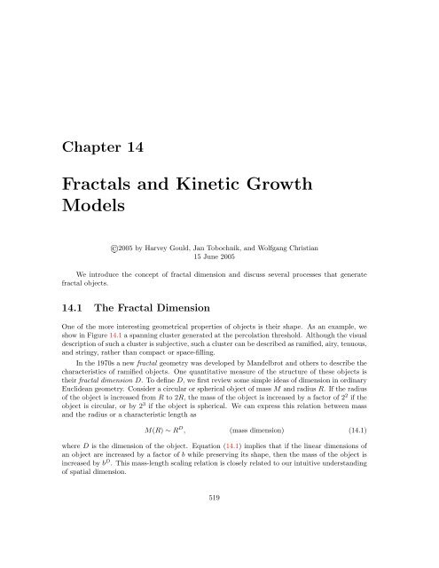
<strong>Chapter</strong> 14Fractals and Kinetic GrowthModels©2005 by Harvey Gould, Jan Tobochnik, and Wolfgang Christian15 June 2005We introduce the concept of fractal dimension and discuss several processes that generatefractal objects.14.1 The Fractal DimensionOne of the more interesting geometrical properties of objects is their shape. As an example, weshow in Figure 14.1 a spanning cluster generated at the percolation threshold. Although the visualdescription of such a cluster is subjective, such a cluster can be described as ramified, airy, tenuous,and stringy, rather than compact or space-filling.In the 1970s a new fractal geometry was developed by Mandelbrot and others to describe thecharacteristics of ramified objects. One quantitative measure of the structure of these objects istheir fractal dimension D. To define D, we first review some simple ideas of dimension in ordinaryEuclidean geometry. Consider a circular or spherical object of mass M and radius R. If the radiusof the object is increased from R to 2R, the mass of the object is increased by a factor of 2 2 if theobject is circular, or by 2 3 if the object is spherical. We can express this relation between massand the radius or a characteristic length asM(R) ∼ R D , (mass dimension) (14.1)where D is the dimension of the object. Equation (14.1) implies that if the linear dimensions ofan object are increased by a factor of b while preserving its shape, then the mass of the object isincreased by b D . This mass-length scaling relation is closely related to our intuitive understandingof spatial dimension.519
CHAPTER 14. FRACTALS AND KINETIC GROWTH MODELS 520Figure 14.1: Example of a spanning percolation cluster generated at p = 0.5927 on a L = 124square lattice. The other occupied sites are not shown.If the dimension of the object, D, and the dimension of the Euclidean space in which theobject is embedded, d, are identical, then the mass density ρ = M/R d scales asρ(R) ∝ M(R)/R d ∼ R 0 , (14.2)that is, its density is constant. An example of a two-dimensional object is shown in Figure 14.2.An object whose mass-length relation satisfies (14.1) with D = d is said to be compact.Equation (14.1) can be generalized to define the fractal dimension. We denote objects asfractals if they satisfy (14.1) with a value of D different from the spatial dimension d. If an objectsatisfies (14.1) with D < d, its density is not the same for all R, but scales asρ(R) ∝ M/R d ∼ R D−d . (14.3)Because D < d, we see that a fractal object becomes less dense at larger length scales. The scaledependence of the density is a quantitative measure of the ramified or stringy nature of fractalobjects. In addition, another characteristic of fractal objects is that they have holes of all sizes.This property follows from (14.3) because if we replace R by Rb, where b is some constant, weobtain the same power law dependence for ρ(R). Thus, it does not matter what scale of length isused, and thus all hole sizes must be present.Another important characteristic of fractal objects is that they look the same over a rangeof length scales. This property of self-similarity or scale invariance means that if we take part ofa fractal object and magnify it by the same magnification factor in all directions, the magnifiedpicture is similar to the original. This property follows from the scaling argument given for ρ(R).
CHAPTER 14. FRACTALS AND KINETIC GROWTH MODELS 522c. If you have not already done Problem <strong>13</strong>.8a, compute D by determining the mean size (mass)M of the spanning cluster at p = p c as a function of the linear dimension L of the lattice.Consider L = 11, 21, 41, and 61 and estimate D from a log-log plot of M versus L.∗ Problem 14.2. Renormalization group calculation of the fractal dimensionCompute ⟨M 2 ⟩, the average of the square of the number of occupied sites in the spanning clusterat p = p c , and the quantity ⟨M ′2 ⟩, the average of the square of the number of occupied sites in thespanning cluster on the renormalized lattice of linear dimension L ′ = L/b. Because ⟨M 2 ⟩ ∼ L 2Dand ⟨M ′2 ⟩ ∼ (L/b) 2D , we can obtain D from the relation b 2D = ⟨M 2 ⟩/⟨M ′2 ⟩. Choose the lengthrescaling factor to be b = 2 and adopt the same blocking procedure as was used in Section <strong>13</strong>.5. Anaverage over ten spanning clusters for L = 16 and p = 0.5927 is sufficient for qualitative results.In Problems 14.1 and 14.2 we were interested only in the properties of the spanning clusters.For this reason, our algorithm for generating percolation configurations by randomly occupyingeach site is inefficient because it generates many clusters. A more efficient way of generatingsingle percolation clusters is due independently to Hammersley, Leath, and Alexandrowicz. Thisalgorithm, commonly known as the Leath or the single cluster growth algorithm, is equivalent tothe following steps (see Figure 14.3):1. Occupy a single seed site on the lattice. The nearest neighbors (four on the square lattice)of the seed represent the perimeter sites.2. For each perimeter site, generate a uniform random number r in the unit interval. If r ≤ p,the site is occupied and added to the cluster; otherwise the site is not occupied. In orderthat sites be unoccupied with probability 1 − p, these sites are not tested again.3. For each site that is occupied, determine if there are any new perimeter sites, that is, untestedneighbors. Add the new perimeter sites to the perimeter list.4. Continue steps 2 and 3 until there are no untested perimeter sites to test for occupancy.Class SingleCluster implements this algorithm and computes the number of occupied siteswithin a radius r of the seed particle. The seed site is placed at the center of a square lattice.Two one-dimensional arrays, pxs and pys, store the x and y positions of the perimeter sites.The status of a site is stored in the byte array s with s(x,y) = (byte) 1 for an occupied site,s(x,y) = (byte) 2 for a perimeter site, and s(x,y) = (byte)-1 for a site that has already beentested and not occupied, and s(x,y) = (byte) 0 for an untested and unvisited site. To avoidchecking for the boundaries of the lattice, we add extra rows and columns at the boundaries andset these sites equal to (byte)-1. We use a byte array because the array s will be sent to theLatticeFrame class which uses byte arrays.Listing 14.1: Class SingleCluster generates and analyzes a single percolation cluster.package org . o p e n s o u r c e p h y s i c s . s i p . ch<strong>13</strong> . c l u s t e r ;public class S i n g l e C l u s t e r {public byte s i t e [ ] [ ] ;public int [ ] xs , ys , pxs , pys ;
CHAPTER 14. FRACTALS AND KINETIC GROWTH MODELS 523ggggxggggxggggggxggggggggggggggggggggxgxxggxgxggxgxggxggFigure 14.3: An example of the growth of a percolation cluster. Sites are occupied with probabilityp. Occupied sites are represented by a shaded square, growth or perimeter sites are labeled by g,and tested unoccupied sites are labeled by x. Because the seed site is occupied but not tested,we have represented it differently than the other occupied sites. The growth sites are chosen atrandom.public int L ;public double p ; // s i t e occupation p r o b a b i l i t yint occupiedNumber ;int perimeterNumber ;int nx [ ] = {1 , −1, 0 , 0 } ; // r e l a t i v e change in x to n e a r e s t n e i g h b o r sint ny [ ] = {0 , 0 , 1 , −1}; // r e l a t i v e change in y to n e a r e s t n e i g h b o r sdouble mass [ ] ; // mass o f ring , index i s d i s t a n c e from c e n t e r o f masspublic void i n i t i a l i z e ( ) {s i t e = new byte [ L+2][L+2]; // g i v e s s t a t u s o f each s i t exs = new int [ L*L ] ; // l o c a t i o n o f occupied s i t e sys = new int [ L*L ] ;pxs = new int [ L*L ] ; // l o c a t i o n o f perimeter s i t e spys = new int [ L*L ] ;for ( int i = 0 ; i
CHAPTER 14. FRACTALS AND KINETIC GROWTH MODELS 524}pys [ n ] = ys [0]+ ny [ n ] ;s i t e [ pxs [ n ] ] [ pys [ n ] ] = ( byte ) 2 ;}perimeterNumber = 4 ;public void s t e p ( ) {i f ( perimeterNumber >0) {int p e r i m e t e r = ( int ) (Math . random ( ) * perimeterNumber ) ;int x = pxs [ p e r i m e t e r ] ;int y = pys [ p e r i m e t e r ] ;perimeterNumber −−;pxs [ p e r i m e t e r ] = pxs [ perimeterNumber ] ;pys [ p e r i m e t e r ] = pys [ perimeterNumber ] ;i f (Math . random()
CHAPTER 14. FRACTALS AND KINETIC GROWTH MODELS 526}plotFrame . append ( 0 , Math . l o g ( r ) , Math . l o g ( massEnclosed ) ) ;r P r i n t *= 2 ;}}plotFrame . s e t V i s i b l e ( true ) ;public void r e s e t ( ) {c o n t r o l . setValue ( "L" , 6 1 ) ;c o n t r o l . setValue ( "p" , 0 . 5 9 2 7 ) ;s e t S t e p s P e r D i s p l a y ( 1 0 ) ;enableStepsPerDisplay ( true ) ;}}public s t a t i c void main ( S t r i n g [ ] a r g s ) {SimulationControl . createApp (new SingleClusterApp ( ) ) ;}We will use the Leath or single cluster growth algorithm in Problem 14.3 to generate a spanningcluster at the percolation threshold. The fractal dimension is determined by counting the numberof sites M in the cluster within a distance r of the center of mass of the cluster. The center ofmass is defined byr cm = 1 ∑r i , (14.4)Nwhere N is the total number of particles in the cluster. A typical plot of ln M(r) versus ln r isshown in Figure 14.4. Because the cluster cannot grow past the edge of the lattice, we do notinclude data for r ≈ L.Problem 14.3. Single cluster growth and the fractal dimensiona. Explain how the Leath algorithm generates single clusters in a way that is equivalent to themultiple clusters that are generated by visiting all sites. More precisely, the Leath algorithmgenerates percolation clusters with a distribution of cluster sizes equal to sn s . For example, ifyou grow 10 clusters of size s = 2, then n s = 10/2 = 5. The additional factor of s is due to thefact that each site of the cluster has an equal chance of being the seed of the cluster, and hencethe same cluster can be generated in s ways.b. Grow as large a spanning cluster as you can and look at it on different length scales. Oneway to do so is to divide the screen into four windows, each of which magnifies a part of thecluster shown in the previous window. Does the part of the cluster shown in each window lookapproximately self-similar?c. Choose p = 0.5927 and L ≥ 61 and generate at least ten configurations of spanning clusters.Determine the number of occupied sites M(r) within a distance r of the seed site of each cluster.(Better results can be found by choosing the origin to be the center of mass of each cluster.)Average M(r) over the spanning clusters. Estimate D from the log-log plot of M versus r (seeFigure 14.4). If time permits, generate percolation clusters on larger lattices.i
CHAPTER 14. FRACTALS AND KINETIC GROWTH MODELS 527108ln M64200 1 2 3 4 5ln rFigure 14.4: Plot of ln M versus ln r for a single spanning percolation cluster generated at p =0.5927 on a L = 129 square lattice. The straight line is a linear least squares fit to the data. Theslope of this line is 1.91 and is an estimate of the fractal dimension D. The exact value of D for apercolation cluster at p = p c in two dimensions is D = 91/48 ≈ 1.896.d. Generate clusters at p = 0.65, a value of p greater than p c , for L = 101. Make a log-log plot ofM(r) versus r. Is the slope approximately equal to the value of D found in part (c)? Does theslope increase or decrease for larger r? Repeat for p = 0.80. Is a spanning cluster generated atp > p c a fractal?e. The fractal dimension of percolation clusters is not an independent exponent, but satisfies thescaling relation,D = d − β/ν, (14.5)where β and ν are defined in Table <strong>13</strong>.1. The relation (14.5) can be understood by the followingfinite-size scaling argument. The number of sites in the spanning cluster on a lattice of lineardimension L is given byM(L) ∼ P ∞ (L)L d , (14.6)where P ∞ is the probability that an occupied site belongs to the spanning cluster and L d is thetotal number of sites in the lattice. In the limit of an infinite lattice and p near p c , we knowthat P ∞ (p) ∼ (p − p c ) β and ξ(p) ∼ (p − p c ) −ν independent of L. Hence for L ∼ ξ, we have thatP ∞ (L) ∼ L −β/ν (see (<strong>13</strong>.11)), and we can writeM(L) ∼ L −β/ν L d ∼ L D . (14.7)The relation (14.5) follows. Use the exact values of β and ν from Table <strong>13</strong>.1 to find the exactvalue of D for d = 2. Is your estimate for D consistent with this value?
CHAPTER 14. FRACTALS AND KINETIC GROWTH MODELS 528(a)(b)Figure 14.5: The first three stages (a)–(c) of the generation of a self-similar Koch curve. At eachstage the displacement of the middle third of each segment is in the direction that increases thearea under the curve. The curves were generated using Class KochApp. The Koch curve is anexample of a continuous curve for which there is no tangent defined at any of its points. The Kochcurve is self-similar on each length scale.(c)f. ∗ Rewrite the SingleCluster class so that the lattice is stored as a one-dimensional array as isdone for class Clusters in <strong>Chapter</strong> <strong>13</strong>.g. ∗ Estimate the fractal dimension for percolation clusters on a simple cubic lattice. Take p c =0.3117.14.2 Regular FractalsAs we have seen, one characteristic of random fractal objects is that they look the same on arange of length scales. To gain a better understanding of the meaning of self-similarity, considerthe following example of a regular fractal, a mathematical object that is self-similar on all lengthscales. Begin with a line one unit long (see Figure 14.5a). Remove the middle third of the line andreplace it by two lines of length 1/3 each so that the curve has a triangular bump in it and the totallength of the curve is 4/3 (see Figure 14.5b). In the next stage, each of the segments of length 1/3is divided into lines of length 1/9 and the procedure is repeated as shown in Figure 14.5c. Whatis the length of the curve shown in Figure 14.5c?The three stages shown in Figure 14.5 can be extended an infinite number of times. Theresulting curve is infinitely long and contains an infinite number of infinitesimally small segments.Such a curve is known as the triadic Koch curve. A Java class that uses a recursive procedure (seeSection 7.3) to draw this curve is given in Listing 14.3. Note that method iterate calls itself. Useclass KochApp to generate the curves shown in Figure 14.5.Listing 14.3: Class for drawing the Koch curve.package org . o p e n s o u r c e p h y s i c s . s i p . ch<strong>13</strong> ;
CHAPTER 14. FRACTALS AND KINETIC GROWTH MODELS 530d = 1 d = 2Figure 14.6: Examples of one-dimensional and two-dimensional objects.}c o n t r o l . setValue ( "Number of iterations " , 3 ) ;}public s t a t i c void main ( S t r i n g a r g s [ ] ) {C a l c u l a t i o n C o n t r o l . createApp (new KochApp ( ) ) ;}How can we determine the fractal dimension of the Koch and similar mathematical objects?There are several generalizations of the Euclidean dimension that lead naturally to a definition ofthe fractal dimension (see Section 14.5). Here we consider a definition based on counting boxes.Consider a one-dimensional curve of unit length that has been divided into N equal segmentsof length l so that N = 1/l (see Figure 14.6). As l decreases, N increases linearly, which isthe expected result for a one-dimensional curve. Similarly if we divide a two-dimensional squareof unit area into N equal subsquares of length l, we have N = 1/l 2 , the expected result for atwo-dimensional object (see Figure 14.6). In general, we have N = 1/l D , where D is the fractaldimension of the object. If we take the logarithm of both sides of this relation, we can express thefractal dimension asD =log N . (box dimension) (14.8)log(1/l)Now let us apply this definition to the Koch curve. Each time the length l of our measuringunit is reduced by a factor of 3, the number of segments is increased by a factor of 4. If we use thesize of each segment as the size of our measuring unit, then at the nth iteration we have N = 4 nand l = (1/3) n , and the fractal dimension of the triadic Koch curve is given byD =log 4nlog 3 n = n log 4 ≈ 1.2619. (triadic Koch curve) (14.9)n log 3From (14.9) we see that the Koch curve has a fractal dimension between that of a line and a plane.Is this statement consistent with your visual interpretation of the degree to which the triadic Kochcurve fills space?Problem 14.4. The recursive generation of regular fractalsa. Recursion is used in method iterate in KochApp and is one of the more difficult programmingconcepts. Explain the nature of recursion and the way it is implemented .
CHAPTER 14. FRACTALS AND KINETIC GROWTH MODELS 531(a)(b)(c)Figure 14.7: (a) The first few iterations of the quadric Koch curve; (b) The first few iterations ofthe Sierpiński gasket; (c) The first few iterations of the Sierpiński carpet.b. Regular fractals can be generated from a pattern that is used in a self-replicating manner.Write a program to generate the quadric Koch curve shown in Figure 14.7a. What is its fractaldimension?c. What is the fractal dimension of the Sierpiński gasket shown in Figure 14.7b? Write a programthat generates the next several iterations.d. What is the fractal dimension of the Sierpiński carpet shown in Figure 14.7c? How does thefractal dimension of the Sierpiński carpet compare to the fractal dimension of a percolationcluster? Are the two fractals visually similar?14.3 Kinetic Growth ProcessesMany systems in nature exhibit fractal geometry. Fractals have been used to describe the irregularshapes of such varied objects as coastlines, clouds, coral reefs, and the human lung. Why arefractal structures so common? How do fractal structures form? In this section we discuss severalgrowth models that generate structures that show a remarkable similarity to forms observed innature. The first two models are already familiar to us and exemplify the flexibility and utility ofkinetic growth models.Epidemic model. In the context of the spread of disease, we usually want to know theconditions for an epidemic. A simple lattice model of the spread of a disease can be formulated
CHAPTER 14. FRACTALS AND KINETIC GROWTH MODELS 532as follows. Suppose that an occupied site corresponds to an infected person. Initially there is asingle infected person and the four nearest neighbor sites (on the square lattice) correspond tosusceptible people. At the next time step, we visit the four susceptible sites and occupy (infect)each site with probability p. If a susceptible site is not occupied, we say that the site is immuneand we do not test it again. We then find the new susceptible sites and continue until either thedisease is controlled or reaches the boundary of the lattice. Convince yourself that this growthmodel of a disease generates a cluster of infected sites that is identical to a percolation cluster atprobability p. The only difference is that we have introduced a discrete time step into the model.Some of the properties of this model are explored in Problem 14.5.Problem 14.5. A simple epidemic modela. Explain why the simple epidemic model discussed in the text generates the same clusters as inthe percolation model. What is the minimum value of p necessary for an epidemic to occur?Recall that in one time step, all susceptible sites are visited simultaneously and infected withprobability p. Determine how n, the number of infected sites, depends on the time t (thenumber of time steps) for various values of p. A straightforward way to proceed is to modifyclass SingleCluster so that all susceptible sites are visited and occupied with probability pbefore new susceptible sites are found. In <strong>Chapter</strong> 15 we will learn that this model is an exampleof a cellular automaton.b. What are some ways that you could modify the model to make it more realistic? For example,the infected sites might recover after a certain time.Eden model. An even simpler example of a growth model was proposed by Eden in 1958to simulate the growth of tumors or a bacterial colony. Although we will find that the resultantmass distribution is not a fractal, the description of the Eden model illustrates the general natureof the fractal growth models we will discuss.Choose a seed site at the center of the lattice for simplicity. The unoccupied nearest neighborsof the occupied sites are the perimeter or growth sites. In the simplest version of the model, agrowth site is chosen at random and occupied. The newly occupied site is removed from the list ofgrowth sites and the new growth sites are added to the list. This process is repeated many timesuntil a large cluster of occupied sites is formed. The difference between this model and the simpleepidemic model is that all tested sites are occupied. In other words, no growth sites ever become“immune.” Some of the properties of Eden clusters are investigated in Problem 14.6.Problem 14.6. The Eden modela. Modify class SingleCluster so that clusters are generated on a square lattice according tothe Eden model. A straightforward procedure is to occupy perimeter sites with probabilityp = 1. The simulation should be stopped when the cluster just reaches the edge of the lattice.What would happen if we were to occupy perimeter sites indefinitely? Follow the procedure ofProblem 14.3 and determine the number of occupied sites M(r) within a distance r of the seedsite. Assume that M(r) ∼ r D for sufficiently large r, and estimate D from the slope of a log-logplot of M versus r. A typical log-log plot is shown in Figure 14.8 for L = 61. Can you concludefrom your data that Eden clusters are compact?
CHAPTER 14. FRACTALS AND KINETIC GROWTH MODELS 533108ln M64200 1 2 3 4ln rFigure 14.8: Plot of ln M versus ln r for a single Eden cluster generated on a L = 61 square lattice.A least squares fit from r = 2 to r = 32 yields a slope of approximately 2.01.b. Modify your program so that only the perimeter or growth sites are shown. Where are themajority of the perimeter sites relative to the center of the cluster? Grow as big a cluster astime permits.Invasion percolation. A dynamical process known as invasion percolation has been used tomodel the shape of the oil-water interface that occurs when water is forced into a porous mediumcontaining oil. The goal is to use the water to recover as much oil as possible. In this processa water cluster grows into the oil through the path of least resistance. Consider a lattice of sizeL x × L y , with the water (the invader) initially occupying the left edge (see Figure 14.9). Theresistance to the invader is given by assigning to each lattice site a uniformly distributed randomnumbers between 0 and 1; these numbers are fixed throughout the invasion. Sites that are nearestneighbors of the invader sites are the perimeter sites. At each time step, the perimeter site withthe lowest random number is occupied by the invader and the oil (the defender) is displaced. Theinvading cluster grows until a path of occupied sites connects the left and right edges of the lattice.After this path forms, there is no need for the water to occupy any additional sites. To minimizeboundary effects, periodic boundary conditions are used for the top and bottom edges and allquantities are measured only over a central region for from the left and right edges of the lattice.Class Invasion implements the invasion percolation algorithm. The two-dimensional arrayelement site[i][j] initially stores a random number for the site at (i,j). If the site at (i,j)is occupied, then site[i][j] is set equal to 1. If the site at (i,j) is a perimeter site, thensite[i][j] is increased by 2. In this way we know which sites are perimeter sites and the valueof the random number is associated with the perimeter site. A new perimeter site is inserted intoits proper ordered position in the lists perimeterListX and perimeterListY. The perimeter listsare ordered so that the site with the largest random number is at the beginning.
CHAPTER 14. FRACTALS AND KINETIC GROWTH MODELS 5340.55 0.22 0.61 0.34 0.720.70 0.<strong>13</strong> 0.04 0.89 0.590.10 0.07 0.84 0.42 0.64t = 00.55 0.22 0.61 0.34 0.720.70 0.<strong>13</strong> 0.04 0.89 0.590.10 0.07 0.84 0.42 0.64t = 10.55 0.22 0.61 0.34 0.720.70 0.<strong>13</strong> 0.04 0.89 0.590.10 0.07 0.84 0.42 0.64t = 20.55 0.22 0.61 0.34 0.720.70 0.<strong>13</strong> 0.04 0.89 0.590.10 0.07 0.84 0.42 0.64t = 30.55 0.22 0.61 0.34 0.720.70 0.<strong>13</strong> 0.04 0.89 0.590.10 0.07 0.84 0.42 0.64t = 40.55 0.22 0.61 0.34 0.720.70 0.<strong>13</strong> 0.04 0.89 0.590.10 0.07 0.84 0.42 0.64t = 50.55 0.22 0.61 0.34 0.720.70 0.<strong>13</strong> 0.04 0.89 0.590.10 0.07 0.84 0.42 0.64t = 60.55 0.22 0.61 0.34 0.720.70 0.<strong>13</strong> 0.04 0.89 0.590.10 0.07 0.84 0.42 0.64t = 7Figure 14.9: Example of a cluster formed by invasion percolation on a 5 × 3 lattice. The lattice att = 0 shows the random numbers that have been assigned to the sites. The darkly shaded sites areoccupied by the invader that occupies the perimeter site (lightly shaded) with the smallest randomnumber. The cluster continues to grow until a site in the right-most column is occupied.Two search methods are provided for determining the position of a new perimeter site inthe perimeter lists. In a linear search we go through the list in order until the random numberassociated with the new perimeter site is between two random numbers in the list. In a binarysearch we divide the list in two, and determine in which half the new random number belongs.
CHAPTER 14. FRACTALS AND KINETIC GROWTH MODELS 535Then we divide this half into half again and so on until the correct position is found. The linear andbinary search methods are compared in Problem 14.7d. The binary search is the default methodused in class Invasion.The main quantities of interest are the fraction of sites occupied by the invader, and theprobability P (r)∆r that a site with a random number between r and r + ∆r is occupied. Theproperties of invasion percolation are explored in Problem 14.7.Listing 14.4: Class for simulating invasion percolation.package org . o p e n s o u r c e p h y s i c s . s i p . ch<strong>13</strong> . i n v a s i o n ;import java . awt . Color ;import org . o p e n s o u r c e p h y s i c s . frames . * ;public class I n v a s i o n {public int Lx , Ly ;public double s i t e [ ] [ ] ;public int perimeterListX [ ] , perimeterListY [ ] ;public int numberOfPerimeterSites ;public boolean ok = true ;public LatticeFrame l a t t i c e ;public I n v a s i o n ( LatticeFrame l a t t i c e F r a m e ) {l a t t i c e = l a t t i c e F r a m e ;l a t t i c e . setIndexedColor ( 0 , Color . blue ) ;l a t t i c e . setIndexedColor ( 1 , Color . black ) ;}public void i n i t i a l i z e ( ) {Lx = 2*Ly ;s i t e = new double [ Lx ] [ Ly ] ;perimeterListX = new int [ Lx*Ly ] ;perimeterListY = new int [ Lx*Ly ] ;for ( int y = 0 ; y
CHAPTER 14. FRACTALS AND KINETIC GROWTH MODELS 53911/30 1/31/3t = 0t = 11/181/61/61/180002/3 05/180 7/1802/9t = 2t = 3Figure 14.10: The evolution of the probability distribution function W t (i) for three successive timesteps.displacement ⟨R 2 (t)⟩. How does ⟨R 2 (t)⟩ depend on p and t? We consider this question in Problem14.8.Problem 14.8. The ant in the labyrintha. For p = 1, the ants walk on a perfect lattice, and hence, ⟨R 2 (t)⟩ = 2dDt. Suppose that anant does a random walk on a spanning cluster with p > p c on a square lattice. Assume that⟨R 2 (t)⟩ → 4D s (p) t for p > p c and sufficiently long times. We have denoted the diffusioncoefficient by D s because we are considering random walks only on spanning clusters and arenot considering walks on the finite clusters that also exist for p > p c . Generate a cluster atp = 0.7 using the single cluster growth algorithm considered in Problem 14.3. Choose the initialposition of the ant to be the seed site and modify your program to observe the motion of theant on the screen. Use L ≥ 101 and average over at least 100 walkers for t up to 500. Wheredoes the ant spend much of its time? If ⟨R 2 (t)⟩ ∝ t, what is D s (p)/D(p = 1)?b. As in part (a) compute ⟨R 2 (t)⟩ for p = 1.0, 0.8, 0.7, 0.65, and 0.62 with L = 101. If timepermits, average over several clusters. Make a log-log plot of ⟨R 2 (t)⟩ versus t. What is thequalitative t-dependence of ⟨R 2 (t)⟩ for relatively short times? Is ⟨R 2 (t)⟩ proportional to t forlonger times? (Remember that the maximum value of ⟨R 2 ⟩ is bounded by the finite size of thelattice.) If ⟨R 2 (t)⟩ ∝ t, estimate D s (p). Plot D s (p)/D(p = 1) as a function of p and discuss itsqualitative dependence.c. Compute ⟨R 2 (t)⟩ for p = 0.4 and confirm that for p < p c , the clusters are finite, ⟨R 2 (t)⟩ isbounded, and diffusion is impossible.
CHAPTER 14. FRACTALS AND KINETIC GROWTH MODELS 540d. Because there is no diffusion for p < p c , we might expect that D s vanishes as p → p c fromabove, that is, D s (p) ∼ (p − p c ) µs for p p c . Extend your calculations of part (b) to larger L,more walkers (at least 1000) and more values of p near p c and estimate the dynamical exponentµ s .e. At p = p c , we might expect ⟨R 2 (t)⟩ to exhibit a different type of t-dependence, for example,⟨R 2 (t)⟩ → t 2/z for large t. Do you expect the exponent z to be greater or less than two? Doa simulation of ⟨R 2 (t)⟩ at p = p c and estimate z. Choose L ≥ 201 and average over severalspanning clusters.f. The algorithm we have been using corresponds to a “blind” ant, because the ant chooses fromfour outcomes even if some of these outcomes are not possible. In contrast, the “myopic” antcan look ahead and see the number q of nearest neighbor occupied sites. The ant then choosesone of the q possible outcomes and thus always takes a step. Redo the simulations in part (b).Does ⟨R 2 (t)⟩ reach its asymptotic linear dependence on t earlier or later compared to the blindant?g. ∗ The limitation of approach we have taken so far is that we have to average over differentrandom walks R 2 (t) on a given cluster and also average over different clusters. A more efficientway of treating random walks on a random lattice is to use an exact enumeration approach andto consider all possible walks on a given cluster. The idea of the exact enumeration methodis that W t+1 (i), the probability that the ant is at site i at time t + 1, is determined solely bythe probabilities of the ant being at the neighbors of site i at time t. Store the positions ofthe occupied sites in an array and introduce two arrays corresponding to W t+1 (i) and W t (i)for all sites i in the cluster. Use the probabilities W t (i) to obtain W t+1 (i) (see Figure 14.10).Spatial averages such as the mean square displacement can be calculated from the probabilitydistribution function at different times. The details of the method and the results are discussedin Majid et al., where walks of 5000 steps on clusters with ∼ 10 3 sites and averaged their resultsover 1000 different clusters.h. ∗ Another reason for the interest in diffusion in disordered media is that the diffusion coefficient isproportional to the electrical conductivity of the medium. One of Einstein’s many contributionswas to show that the mobility, the ratio of the mean velocity of the particles in a system to anapplied force, is proportional to the self-diffusion coefficient in the absence of the applied force(see Reif). For a system of charged particles, the mean velocity of the particles is proportionalto the electrical current and the applied force is proportional to the voltage. Hence the mobilityand the electrical conductivity are proportional, and the conductivity is proportional to theself-diffusion coefficient.The electrical conductivity σ vanishes near the percolation threshold as σ ∼ (p−p c ) µ , withµ ≈ 1.30 (see Section <strong>13</strong>.1). The difficulty of doing a direct Monte Carlo calculation of σ wasconsidered in Project <strong>13</strong>.18. We measured the self-diffusion coefficient D s by always placingthe ant on a spanning cluster rather than on any cluster. In contrast, the conductivity ismeasured for the entire system including all finite clusters. Hence, the self-diffusion coefficientD that enters into the Einstein relation should be determined by placing the ant at randomanywhere on the lattice, including sites that belong to the spanning cluster and sites thatbelong to the many finite clusters. Because only those ants that start on the spanning cluster
CHAPTER 14. FRACTALS AND KINETIC GROWTH MODELS 541Figure 14.11: A DLA cluster of 4284 particles on a square lattice with L = 300.can contribute to D, D is related to D s by D = P ∞ D s , where P ∞ is the probability that theant would land on a spanning cluster. Because P ∞ scales as P ∞ ∼ (p − p c ) β , we have that(p − p c ) µ ∼ (p − p c ) β (p − p c ) µs or µ = µ s + β. Use your result for µ s found in part (d) and theexact result β = 5/36 (see Table <strong>13</strong>.1) to estimate µ and compare your result to the criticalexponent µ for the dc electrical conductivity.i. ∗ We also can derive the scaling relation z = 2 + µ s /ν = 2 + (µ − β)ν, where z is defined inpart (e). Is it easier to determine µ s or z accurately from a Monte Carlo simulation on a finitelattice? That is, if your real interest is estimating the best value of the critical exponent µfor the conductivity, should you determine the conductivity directly or should we measure theself-diffusion coefficient at p = p c or at p > p c ? What is your best estimate of the conductivityexponent µ?Diffusion-limited aggregation. Many objects in nature grow by the random addition ofsubunits. Examples include snow flakes, lightning, crack formation along a geological fault, and thegrowth of bacterial colonies. Although it might seem unlikely that such phenomena have much incommon, the behavior observed in many models gives us clues that these and many other naturalphenomena can be understood in terms of a few unifying principles. A popular model that is agood example of how random motion can give rise to beautiful self-similar clusters is known asdiffusion limited aggregation or DLA.The first step is to occupy a site with a seed particle. Next, a particle is released at randomfrom a point on the circumference of a large circle whose center coincides with the seed. Theparticle undergoes a random walk until it reaches a perimeter site of the seed and sticks. Thenanother random walker is released from the circumference of a large circle and walks until it reachesa perimeter site of one of the two particles in the cluster and sticks. This process is repeated manytimes (typically on the order of several thousand to several million) until a large cluster is formed.A typical DLA cluster is shown in Figure 14.11. Some of the properties of DLA clusters areexplored in Problem 14.9.
CHAPTER 14. FRACTALS AND KINETIC GROWTH MODELS 542The following class provides a reasonably efficient simulation of DLA. Walkers begin justoutside a circle of radius startRadius enclosing the existing cluster and centered at the seed site.If the walker moves away from the cluster, the step size for the random walker increases. If thewalker wonders too far away (further than maxRadius), the walk is restarted.Listing 14.5: Class for simulating diffusion limited aggregation.package org . o p e n s o u r c e p h y s i c s . s i p . ch<strong>13</strong> ;import org . o p e n s o u r c e p h y s i c s . c o n t r o l s . * ;import org . o p e n s o u r c e p h y s i c s . frames . LatticeFrame ;import java . awt . Color ;public class DLAApp extends AbstractSimulation {LatticeFrame l a t t i c e F r a m e = new LatticeFrame ( "DLA" ) ;byte s [ ] [ ] ; // l a t t i c e on which c l u s t e r l i v e sint xOccupied [ ] , yOccupied [ ] ; // l o c a t i o n o f occupied s i t e sint L ; // l i n e a r dimension o f l a t t i c eint h a l f L ; // L/2int r i n g S i z e ; // r i n g s i z e in which w a l k e r s can moveint numberOfParticles ; // number o f p a r t i c l e s in c l u s t e rint s t a r t R a d i u s ; // r a d i u s o f c l u s t e r at which w a l k e r s are s t a r t e dint maxRadius ; // maximum r a d i u s walker can go to b e f o r e a new walk i s s t a rpublic void i n i t i a l i z e ( ) {l a t t i c e F r a m e . setMessage ( null ) ;numberOfParticles = 1 ;L = c o n t r o l . g e t I n t ( " lattice size" ) ;s t a r t R a d i u s = 3 ;h a l f L = L/2;r i n g S i z e = L/ 1 0 ;maxRadius = s t a r t R a d i u s+r i n g S i z e ;s = new byte [ L ] [ L ] ;s [ h a l f L ] [ h a l f L ] = Byte .MAX VALUE;l a t t i c e F r a m e . s e t A l l ( s ) ;}public void r e s e t ( ) {l a t t i c e F r a m e . setIndexedColor ( 0 , Color .BLACK) ;c o n t r o l . setValue ( " lattice size" , 3 0 0 ) ;s e t S t e p s P e r D i s p l a y ( 1 0 0 ) ;enableStepsPerDisplay ( true ) ;i n i t i a l i z e ( ) ;}public void stopRunning ( ) {c o n t r o l . p r i n t l n ( "Number of particles = "+numberOfParticles ) ;// add code to compute t h e mass d i s t r i b u t i o n here}public void doStep ( ) {int x = 0 , y = 0 ;
CHAPTER 14. FRACTALS AND KINETIC GROWTH MODELS 543}i f ( startRadius =h a l f L ) { // s t o p t h e s i m u l a t i o nc o n t r o l . c a l c u l a t i o n D o n e ( "Done" ) ;l a t t i c e F r a m e . setMessage ( "Done" ) ;}l a t t i c e F r a m e . setMessage ( "n = "+numberOfParticles ) ;public boolean walk ( int x , int y ) {do {double rSquared = ( x−halfL ) * ( x−h a l f L )+(y−h a l f L ) * ( y−h a l f L ) ;int r = 1+( int ) Math . s q r t ( rSquared ) ;i f ( r>maxRadius ) {return true ; // s t a r t new walker}i f ( ( r0)) {numberOfParticles++;s [ x ] [ y ] = 1 ;l a t t i c e F r a m e . setValue ( x , y , Byte .MAX VALUE) ;i f ( r>=s t a r t R a d i u s ) {s t a r t R a d i u s = r +2;}maxRadius = s t a r t R a d i u s+r i n g S i z e ;return f a l s e ; // walk i s f i n i s h e d} else { // t a k e a s t e pswitch ( ( int ) (4*Math . random ( ) ) ) { // s e l e c t d i r e c t i o n randomlycase 0 :x++;break ;case 1 :x−−;break ;case 2 :y++;break ;case 3 :y−−;}} // end e l s e i f} while ( true ) ; // end do l o o p}public s t a t i c void main ( S t r i n g [ ] a r g s ) {
CHAPTER 14. FRACTALS AND KINETIC GROWTH MODELS 544}}SimulationControl . createApp (new DLAApp ( ) ) ;Problem 14.9. Diffusion limited aggregationa. DLAApp generates diffusion limited aggregation clusters on a square lattice. Each walker beginsat a random site on a launching circle of radius r = R max + 2, where R max is the maximumdistance of any particle in the cluster from the origin. To save computer time, we remove awalker that reaches a distance 2R max from the seed site and place a new walker at random onthe circle of radius r. If the clusters appear to be fractals, make a visual estimate of the fractaldimension. Choose a lattice of linear dimension L ≥ 61. (Experts can make a visual estimateof D to within a few percent.) Modify DLAApp by color coding the sites in the cluster accordingto their time of arrival, for example, color the first group of sites white, the next group blue,the next group red, and the last group green. (Your choice of the size of the group depends inpart on the total size of your cluster.) Which parts of the cluster grow faster? Do any of thelate arriving green particles reach the center?b. At t = 0 the four perimeter (growth) sites on the square lattice each have a probability p i = 1/4of becoming part of the cluster. At t = 1, the cluster has mass two and six perimeter sites.Identify the perimeter sites and convince yourself that their growth probabilities are not thesame. Do a Monte Carlo simulation and verify that two perimeter sites have growth probabilitiesp = 2/9 and the other four have p = 5/36. We discuss a more direct way of determining thegrowth probabilities in Problem 14.10.c. DLAApp generates clusters inefficiently, because most of the CPU time is spent while the randomwalker is wandering far from the perimeter sites of the cluster. There are several ways ofmaking your program more efficient. One way is to let the walker take bigger steps the furtherit is from the cluster. For example, if the walker is a distance R > R max , a step of lengthgreater than or equal to R − R max − 1 may be permitted if this distance is greater than onelattice unit. If the walker is very close to the cluster, the step length is one lattice unit. Makethis modification to class DLA and estimate the fractal dimension of diffusion limited clustersgenerated on a square lattice by computing M(r), the number of sites in the cluster within aradius r centered at the seed site. Because very large clusters are needed to accurately estimatethe fractal dimension, you will obtain only approximate results. Other possible modificationsto make in the implementation of the algorithm are discussed in Project 14.17 and by Meakin(see references).d. ∗ Each time we grow a DLA cluster (and other clusters in which a perimeter site is selected atrandom), we obtain a slightly different cluster if we use a different random number sequence.One way of reducing this “noise” is to use “noise reduction,” that is, a perimeter site is notoccupied until it has been visited m times. Each time the random walker lands on a perimetersite, the number of visits for this site is increased by one until the number of visits equalsm and the site is occupied. The idea is that noise reduction accelerates the approach to theasymptotic scaling behavior. Consider m = 2, 3, 4, and 5 and grow DLA clusters on the squarelattice. Are there any qualitative differences between the clusters for different values of m?
CHAPTER 14. FRACTALS AND KINETIC GROWTH MODELS 545e. ∗ In <strong>Chapter</strong> <strong>13</strong> we found that the exponents describing the percolation transition are independentof the symmetry of the lattice, for example, the exponents for the square and triangularlattices are the same. We might expect that the fractal dimension of DLA clusters would alsoshow such universal behavior. However, the presence of a lattice introduces a small anisotropythat becomes apparent only when very large clusters with the order of 10 6 sites are grown.Modify your program so that DLA clusters are generated on a triangular lattice. Do the clustershave the same visual appearance as on the square lattice? Estimate the fractal dimensionand compare your estimate to your result for the square lattice. The best estimates of D forthe square and triangular lattices are D ≈ 1.5 and D ≈ 1.71 respectively. We are remindedof the difficulty of extrapolating the asymptotic behavior from finite clusters. We consider thegrowth of diffusion-limited aggregation clusters in the continuum in Project 14.16.∗ Laplacian growth model. As we discussed in Section 11.6, we can formulate the solutionof Laplace’s equation in terms of a random walk. We now do the converse and formulate theDLA algorithm in terms of a solution to Laplace’s equation. Consider the probability P (r) that arandom walker reaches a site r starting from the external boundary. This probability satisfies therelationP (r) = 1 ∑P (r + a), (14.10)4awhere the sum in (14.10) is over the four nearest neighbor sites (on a square lattice). If we setP = 1 on the boundary and P = 0 on the cluster, then (14.10) also applies to sites that areneighbors of the external boundary and the cluster. A comparison of the form of (14.10) with theform of (11.12) shows that the former is a discrete version of Laplace’s equation, ∇ 2 P = 0. HenceP (r) has the same behavior as the electrical potential between two electrodes connected to theouter boundary and the cluster, and the growth probability at a perimeter site of the cluster isproportional to the value of the potential at that site.∗ Problem 14.10. Laplacian growth modelsa. Solve the discrete Laplace equation (14.10) by hand for the growth probabilities of a DLAcluster of mass 1, 2, and 3. Set P = 1 on the boundary and P = 0 on the cluster. Compareyour results to your results in Problem 14.9b for mass 1 and 2.b. You are probably familiar with the random nature of electrical discharge patterns that occur inatmospheric lightning. Although this phenomenon, known as dielectric breakdown, is complicated,we will see that a simple model leads to discharge patterns that are similar to those thatare observed in nature. Because lightning occurs in an inhomogeneous medium with differencesin the density, humidity, and conductivity of air, we will develop a model of electrical dischargein an inhomogeneous insulator. We know that when an electrical discharge occurs, the electricalpotential ϕ satisfies Laplace’s equation ∇ 2 ϕ = 0. One version of the model (see Family et al.)is specified by the following steps:(i.) Consider a large boundary circle of radius R and place a charge source at the origin.Choose the potential ϕ = 0 at the origin (an occupied site) and ϕ = 1 for sites on thecircumference of the circle. The radius R should be larger than the radius of the growingpattern.
CHAPTER 14. FRACTALS AND KINETIC GROWTH MODELS 546(ii.) Use the relaxation method (see Section 11.5) to compute the values of the potential ϕ ifor (empty) sites within the circle.(iii.) Assign a random number r to each empty site within the boundary circle. The randomnumber r i at site i represents a breakdown coefficient and the random inhomogeneousnature of the insulator.(iv.) The growth sites are the nearest neighbor sites of the discharge pattern (the occupiedsites). Form the product r i ϕ a i for each growth site i, where a is an adjustable parameter.Because the potential for the discharge pattern is zero, ϕ i for growth site i can beinterpreted as the magnitude of the potential gradient at site i.(v.) The perimeter site with the maximum value of the product rϕ a breaks down, that is, setϕ for this site equal to zero.(vi.) Use the relaxation method to recompute the values of the potential at the remainingunoccupied sites and repeat steps (iv) and (v).Choose a = 1/4 and analyze the structure of the discharge pattern. Does the pattern appearqualitatively similar to lightning? Does the pattern appear to have a fractal geometry? Estimatethe fractal dimension by counting M(b), the average number of sites belonging to the dischargepattern that are within a b × b box. Consider other values of a, for example, a = 1/6 anda = 1/3, and show that the patterns have a fractal structure with a tunable fractal dimensionthat depends on the parameter a. Published results (Family et al.) are for patterns with 800occupied sites.c. Another version of the dielectric breakdown model associates a growth probability p i = ϕ a i / ∑ j ϕa jwith each growth site i, where the sum is over all the growth sites. One of the growth sites isoccupied with probability p i . That is, choose a growth site at random and generate a randomnumber r between 0 and 1. If r ≤ p i , the growth site i is occupied. As before, the exponent ais a free parameter. Convince yourself that a = 1 corresponds to diffusion-limited aggregation.(The boundary condition used in the latter corresponds to a zero potential at the growth sites.)To what type of cluster does a = 0 correspond? Consider a = 1/2, 1, and 2 and explore thedependence of the visual appearance of the clusters on a. Estimate the fractal dimension of theclusters.d. Consider a deterministic growth model for which all growth sites are tested for occupancy ateach growth step. Adopt the same geometry and boundary conditions as in part (b) and usethe relaxation method to solve Laplace’s equation for ϕ i . Then find the perimeter site with thelargest value of ϕ and set ϕ max equal to this value. Only those perimeter sites for which theratio ϕ i /ϕ max is larger than a parameter p become part of the cluster; ϕ i is set equal to unityfor these sites. After each growth step, the new growth sites are determined and the relaxationmethod is used to recompute the values of ϕ i at each unoccupied site. Choose p = 0.35 anddetermine the nature of the regular fractal pattern. What is the fractal dimension? Considerother values of p and determine the corresponding fractal dimension. These patterns have beentermed Laplace fractal carpets (see Family et al.).Surface growth models. The fractal objects we have discussed so far are self-similar, thatis, if we look at a small piece of the object and magnify it isotropically to the size of the original,the original and the magnified object look similar (on the average). In the following, we introduce
CHAPTER 14. FRACTALS AND KINETIC GROWTH MODELS 547some simple models that generate a class of fractals that are self-similar only for scale changes incertain directions.Suppose that we have a flat surface at time t = 0. How does the surface grow as a result ofvapor deposition and sedimentation? For example, consider a surface that is initially a line of Loccupied sites. Growth is in the vertical direction only (see Figure 14.12).As before, we simply choose a growth site at random and occupy it (the Eden model again).The average height of the surface is given byh = 1 ∑N sh i , (14.11)N swhere h i is the distance of the ith surface site from the substrate, and the sum is over all surfacesites N s . (The precise definition of a surface site is discussed in Problem 14.11.)Each time a particle is deposited, the time t is increased by unity. Our main interest is howthe width of the surface changes with t. We define the width of the surface byi=1w 2 = 1 ∑N s(h i − h) 2 . (14.12)N si=1In general, the width w, which is a measure of the surface roughness, depends on L and t. Forshort times we expect thatw(L, t) ∼ t β . (14.<strong>13</strong>)The exponent β describes the growth of the correlations with time along the vertical direction.Figure 14.12 illustrates the evolution of the surface generated according to the Eden model.After a characteristic time, the length over which the fluctuations are correlated becomes comparableto L, and the width reaches a steady state value that depends only on L. We writewhere α is known as the roughness exponent.w(L, t ≫ 1) ∼ L α , (14.14)From (14.14) we see that in the steady state, the width of the surface in the direction perpendicularto the substrate grows as L α . This scaling behavior of the width is characteristic ofa self-affine fractal. Such a fractal is invariant (on the average) under anisotropic scale changes,that is, different scaling relations exist along different directions. For example, if we rescale thesurface by a factor b in the horizontal direction, then the surface must be rescaled by a factor ofb α in the direction perpendicular to the surface to preserve the similarity along the original andrescaled surfaces.Note that on short length scales, that is, lengths shorter than the width of the interface, thesurface is rough and its roughness can be characterized by the exponent α. (Imagine an ant walkingon the surface.) For length scales much larger than the width of the surface, the surface appears tobe flat and, in our example, it is a one-dimensional object. The properties of the surface generatedby several growth models are explored in Problem 14.11.Problem 14.11. Growing surfaces
CHAPTER 14. FRACTALS AND KINETIC GROWTH MODELS 548Figure 14.12: Example of surface growth according to the Eden model. The surface site in columni is the perimeter site with the maximum value of h i . In the figure the average height of the surfaceis 20.46 and the width is 2.33.a. In the Eden model a perimeter site is chosen at random and occupied. The growth rule isthe same as the usual Eden model, but the growth is started from a line of length L ratherthan a single site. Hence, there can be “overhangs” as shown in Figure 14.12. Use periodicboundary conditions in the horizontal direction to determine the perimeter sites. The heighth i corresponds to the height of column i. Consider L = 64. Describe the visual appearance ofthe surface as the surface grows. Is the surface well-defined visually? Where are most of theperimeter sites?b. To estimate the exponents α and β, plot the width w(t) as a function of t for L = 32, 64, and128 on the same graph. What type of plot is most appropriate? Does the width initially growas a power law? If so, estimate the exponent β. Is there a L-dependent crossover time afterwhich the width of the surface approaches its steady state value? How can you estimate theexponent α? The best numerical estimates for β and α are consistent with the exact valuesβ = 1/3 and α = 1/2.c. ∗ The dependence of w(L, t) on t and L can be combined into the scaling formwherew(L, t) ≈ L α f(t/L α/β ), (14.15)f(x) ={Ax β x ≪ 1constant, x ≫ 1(14.16)where A is a constant. Verify the existence of the scaling form (14.15) by plotting the ratiow(L, t)/L α versus t/L α/β for the different values of L considered in part (b). If the scalingforms holds, the results for w for the different values of L should fall on a universal curve. Useeither the estimated values of α and β that you found in part (b) or the exact values.d. The Eden model is not really a surface growth model, because any perimeter site can becomepart of the cluster. In the simplest random deposition model, a column is chosen at randomand a particle is deposited at the top of the column of already deposited particles. There isno horizontal correlation between neighboring columns. Do a simulation of this growth modeland visually inspect the surface of the interface. Show that the heights of the columns follow aPoisson distribution (see (8.30)) and that h ∼ t and w ∼ t 1/2 . This structure does not dependon L and hence α = 0.
CHAPTER 14. FRACTALS AND KINETIC GROWTH MODELS 549Figure 14.<strong>13</strong>: Example of the growth of a surface according to the ballistic deposition model. Notethat if column one is chosen, the next site that would be occupied (not shaded) would leave anunoccupied site below it.e. In the ballistic deposition model a column is chosen at random and a particle is assumed tofall vertically until it reaches the first perimeter site that is a nearest neighbor of a site thatalready is part of the surface. This condition allows for growth parallel to the substrate. Onlyone particle falls at a time. How do the rules for this growth model differ from those of theEden model? How does the surface compare to that of the Eden model? Suppose that insteadof the particle falling vertically, we let it do a random walk as in DLA. Would the resultantsurface be the same?14.4 Fractals and ChaosIn <strong>Chapter</strong> 7 we explored dynamical systems that exhibited chaos under certain conditions. Wefound that after an initial transient, the trajectory of such a dynamical system consists of a set ofpoints in phase space called an attractor. For chaotic motion this attractor often is an object thatcan be described as a fractal. Such attractors are called strange attractors.We first consider the familiar logistic map (see (7.1)), x n+1 = 4rx n (1 − x n ). For most valuesof the control parameter r > r ∞ = 0.892486417967 . . . , the trajectories are chaotic. Are thesetrajectories fractals?To calculate the fractal dimension for dynamical systems, we use the box counting methodintroduced in Section 14.2 in which space is divided into d-dimensional boxes of length l. Let N(l)equal the number of boxes that contain a piece of the trajectory. The fractal dimension is definedby the relationN(l) ∼ lim l −D . (box dimension) (14.17)l→0Equation (14.17) holds only when the number of boxes is much larger than N(l) and the numberof points on the trajectory is sufficiently large. If the trajectory moves through many dimensions,that is, the phase space is very large, box counting becomes too memory intensive because we needan array of size ∝ l −d . This array becomes very large for small l and large d.
CHAPTER 14. FRACTALS AND KINETIC GROWTH MODELS 550A more efficient approach is to compute the correlation dimension. In this approach we storein an array the position of N points on the trajectory. We compute the number of points N i (r),and the fraction of points f i (r) = N i (r)/(N − 1) within a distance r of the point i. The correlationfunction C(r) is defined byC(r) ≡ 1 ∑f i (r), (14.18)Nand the correlation dimension D c is defined byiC(r) ∼ limr→0r Dc . (correlation dimension) (14.19)From (14.19) we see that the slope of a log-log plot of C(r) versus r yields an estimate of thecorrelation dimension. In practice, small values of r must be discarded because we cannot sampleall the points on the trajectory, and hence there is a cutoff value of r below which C(r) = 0. In thelarge r limit, C(r) saturates to unity if the trajectory is localized as it is for chaotic trajectories.We expect that for intermediate values of r, there is a scaling regime where (14.19) holds.In Problems 14.12–14.14 we consider the fractal properties of some of the dynamical systemsthat we considered in <strong>Chapter</strong> 7.Problem 14.12. Strange attractor of the logistic mapa. Write a program that uses box counting to determine the fractal dimension of the attractor forthe logistic map. Compute N(l), the number of boxes of length l that have been visited by thetrajectory. Test your program for r < r ∞ . How does the number of boxes containing a piece ofthe trajectory change with l? What does this dependence tell you about the dimension of thetrajectory for r < r ∞ ?b. Compute N(l) for r = 0.9 using at least five different values of l, for example, 1/l = 100, 300,1000, 3000, . . . . Iterate the map at least 10000 times before determining N(l). What is thefractal dimension of the attractor? Repeat for r ≈ r ∞ , r = 0.95, and r = 1.c. Generate points at random in the unit interval and estimate the fractal dimension using thesame method as in part (b). What do you expect to find? Use your results to estimate theaccuracy of the fractal dimension that you found in part (b).d. Write a program to compute the correlation dimension for the logistic map and repeat thecalculations for parts (b) and (c).Problem 14.<strong>13</strong>. Strange attractor of the Hénon mapa. Use two-dimensional boxes of linear dimension l to estimate the fractal dimension of the strangeattractor of the Hénon map (see (7.32)) with a = 1.4 and b = 0.3. Iterate the map at least 1000times before computing N(l). Does it matter what initial condition you choose?b. Compute the correlation dimension for the same parameters used in part (a) and compare D cwith the box dimension computed in part (a).
CHAPTER 14. FRACTALS AND KINETIC GROWTH MODELS 551c. Iterate the Hénon map and view the trajectory on the screen by plotting x n+1 versus x n in onewindow and y n versus x n in another window. Do the two ways of viewing the trajectory looksimilar? Estimate the correlation dimension, where the ith data point is defined by (x i , x i+1 ) andthe distance r ij between the ith and jth data point is given by r ij 2 = (x i −x j ) 2 +(x i+1 −x j+1 ) 2 .d. Estimate the correlation dimension with the ith data point defined by x i , and r ij 2 = (x i − x j ) 2 .What do you expect to obtain for D c ? Repeat the calculation for the ith data point given by(x i , x i+1 , x i+2 ) and r ij 2 = (x i − x j ) 2 + (x i+1 − x j+1 ) 2 + (x i+2 − x j+2 ) 2 . What do you find forD c ?∗ Problem 14.14. Strange attractor of the Lorenz modela. Use three-dimensional graphics or three two-dimensional plots of x(t) versus y(t), x(t) versusz(t), and y(t) versus z(t) to view the structure of the Lorenz attractor. Use σ = 10, b = 8/3,r = 28, and the time step ∆t = 0.01. Compute the correlation dimension for the Lorenzattractor.b. Repeat the calculation of the correlation dimension using x(t), x(t + τ), and x(t + 2τ) insteadof x(t), y(t), and z(t). Choose the delay time τ to be at least ten times greater than the timestep ∆t.c. Compute the correlation dimension in the two-dimensional space of x(t) and x(t + τ). Do thesame calculation in four dimensions using x(t), x(t + τ), x(t + 2τ), and x(t + 3τ). What can youconclude about the results for the correlation dimension using two, three, and four-dimensionalspaces? What do you expect to see for d > 4?Problems 14.<strong>13</strong> and 14.14 illustrate a practical method for determining the underlying structureof systems when, for example, the data consists only of a single time series, that is, measurementsof a single quantity over time. The dimension D c (d) computed by increasing the dimensionof the space, d, using the delayed coordinate τ eventually saturates when d is approximately equalto the number of variables that actually determine the dynamics. Hence, if we have extensive datafor a single variable, for example, the atmospheric pressure or a stock market index, we can usethis method to determine the number of independent variables that determine the dynamics of thevariable. This information can then be used to help create models of the dynamics.14.5 Many DimensionsSo far we have discussed three ways of defining the fractal dimension: the mass dimension (14.1),the box dimension (14.17), and the correlation dimension (14.19). These methods do not alwaysgive the same results for the fractal dimension. Indeed, there are many other dimensions that wecould compute. For example, instead of just counting the boxes that contain a part of an object,we can count the number of points of the object in each box, n i , and compute p i = n i /N, whereN is the total number of points. A generalized dimension D q can be defined asD q = 1q − 1 liml→0ln ∑ N(l)i=1 pq i. (14.20)ln l
CHAPTER 14. FRACTALS AND KINETIC GROWTH MODELS 552The sum in (14.20) is over all the boxes and involves the probabilities raised to the qth power. Forq = 0, we haveln N(l)D 0 = − lim . (14.21)l→0 ln lIf we compare the form of (14.21) with (14.17), we can identify D 0 with the box dimension. Forq = 1, we need to take the limit of (14.20) as q → 1. Letu(q) = ln ∑ ip i q , (14.22)and do a Taylor-series expansion of u(q) about q = 1. We haveu(q) = u(1) + (q − 1) dudq + . . . (14.23)The quantity u(1) = 0 because ∑ i p i = 1. The first derivative of u(q) is given by∑dudq = i p i q ln p∑ ii p i q = ∑ p i ln p i , (14.24)iwhere the last equality follows by setting q = 1. If we use the above relations, we find that D 1 isgiven by∑iD 1 = limp i ln p i. (information dimension) (14.25)l→0 ln lD 1 is called the information dimension because of the similarity of the p ln p term in the numeratorof (14.24) to the information form of the entropy.It is possible to show that D 2 as defined by (14.20) is the same as the mass dimension defined in(14.1) and the correlation dimension D c . That is, box counting gives D 0 and correlation functionsgive D 2 (cf. Sander et al.).There are many objects in nature that differ in appearance but have similar fractal dimension.An example is the different visual appearance in three dimensions of diffusion-limited aggregationclusters and the percolation clusters at the percolation threshold. (Both objects have a fractaldimension of approximately 2.5.) In some cases this difference can be accounted for by the multifractalproperties of an object. For multifractals the various D q are different, in contrast tomonofractals for which the different measures are the same. Percolation clusters are an exampleof a monofractal, because p i ∼ l D0 , the number of boxes N(l) ∼ l −D0 , and from (14.20), D q = D 0for all q. Multifractals occur when the growth quantities are not the same throughout the object,as frequently happens for the strange attractors produced by chaotic dynamics. Diffusion-limitedaggregation is an example of a multifractal.14.6 ProjectsAlthough the kinetic growth models we have considered yield beautiful pictures, there is much wedo not understand. For example, the fractal dimension of DLA clusters can be calculated only byapproximate theories whose accuracy is unknown. Why do the fractal dimensions have the values
CHAPTER 14. FRACTALS AND KINETIC GROWTH MODELS 553that we estimated by various simulations? Can we trust our numerical estimates of the variousexponents, or is it necessary to consider much larger systems to obtain their true asymptotic values?Can we find unifying features for the many kinetic growth models that presently exist? What isthe relation of the various kinetic growth models to physical systems? What are the essentialquantities needed to characterize the geometry of an object?One of the reasons that kinetic growth models are difficult to understand is that the finalcluster typically depends on the history of the growth. We say that these models are examplesof “nonequilibrium behavior.” The combination of simplicity, beauty, complexity, and relevanceto many experimental systems suggests that the study of fractal objects will continue to involve awide range of workers in many disciplines.Project 14.15. The percolation cluster size distributionUse the Leath algorithm to determine the critical exponent τ of the cluster size distribution, n s ,for percolation clusters at p = p c :n s ∼ s −τ . (s ≫ 1) (14.26)Modify class SingleCluster so that many clusters are generated and n s is computed for a givenprobability p. Remember that the number of clusters of size s that are grown from a seed is theproduct sn s , rather than n s itself (see Problem 14.3a). Grow at least 100 clusters on a squarelattice with L ≥ 61. If time permits, use bigger lattices and average over more clusters, and alsoestimate the accuracy of your estimate of τ. See Grassberger for a discussion of an extension ofthis approach to estimating the value of p c in higher dimensions.Project 14.16. Continuum DLAa. In the continuum (off-lattice) version of diffusion-limited aggregation. the diffusing particlesare assumed to be disks of radius a. A disk executes a random walk until its center is withina distance 2a of the center of a disk that is already part of the DLA cluster. At each stepthe walker changes its position by (r cos θ, r sin θ), where r is the step size, and θ is a randomvariable between 0 and 2π. Modify your DLA program or class DLAApp to simulate continuumDLA.b. Compare the appearance of a continuum DLA cluster with a DLA cluster generated on asquare lattice. It is necessary to grow very large clusters (approximately 10 6 particles) to seethe differences.c. Use the mass dimension to estimate the fractal dimension of continuum DLA clusters andcompare its value with the value you found for the square lattice.Project 14.17. More efficient simulation of DLATo improve the efficiency of the algorithm, the walker in class DLAApp is restarted if it wonders toofar from the existing cluster. When the walker is within the distance startRadius of the seed,no optimization is used. Because there can be many unoccupied sites within this distance, it isdesirable to use an additional optimization technique (see Ball and Brady). The idea is to choose
CHAPTER 14. FRACTALS AND KINETIC GROWTH MODELS 554a simple geometrical object (a circle or square) centered at the walker such that none of the clusteris within the object. The walker moves in one step to a site on the boundary of the object. Fora circle the walker can move to any location with equal probability on the circumference. Forthe square we need the probability of moving to various locations on the boundary. To find thelargest object that does not contain a part of the DLA cluster, consider coarse grained lattices.For example, each 2 × 2 group of sites on the original lattice corresponds to one site on the coarserlattice; each 2 × 2 group of sites on the coarse lattice corresponds to a site on an even coarserlattice, etc. If a site is occupied, then any coarse grained site containing this site also is occupied.a. Because we have considered DLA clusters on a square lattice, we use squares centered at thewalker. We first find the probability p(∆x, ∆y, s) that a walker centered on a square of lengthl = 2s + 1, will be displaced by the (∆x, ∆y). This probability can be computed by simulatinga random walk starting at the origin and ending at a boundary site of the square. Repeat thissimulation for many walkers, and then for various values of s. The fraction of walkers thatreach the position (∆x, ∆y) is p(∆x, ∆y, s). Determine p(∆x, ∆y, s) for s = 1 to 16. Store yourresults in a file.b. We next determine the arrays such that for a given value of s and a uniform random numberr, we can quickly find (∆x, ∆y). One way to do so is to create four arrays. The first array liststhe probability determined from part (a) such that the values for s = 1 are listed first. Call thisarray p. For example, p[1] = p(−1, −1, 1), p(2) = p(1)+p(−1, 0, 1), p[3] = p[2]+p(−1, 1, 1),etc. The array start tells us where to start in the array p for each value of s. The arraysdx(i) and dy(i) give the values of ∆x and ∆y corresponding to p[i]. To see how these arraysare used, consider a walker located at (x, y), centered on a square of linear dimension 2s + 1.Generate a random number r and find i = start(s). If r < p[i], then the walker moves to(x + dx(i), y + dy(i)). If not, increment i by unity and check again. Repeat until r ≤ p[i].Write a program to create these four arrays and store them in a file.c. Write a method to determine the maximum value of the parameter s such that a square of size2s + 1 centered at the position of the walker does not contain any part of the DLA cluster. Usecoarse grained lattices to do this determination more efficiently. Modify class DLA to incorporatethis method and the arrays defined part (b). How much faster is your modified program thanthe original class DLA for clusters of 500 and 5000 particles?d. What is the largest cluster you can grow on your computer in a reasonable time? Does thecluster show any evidence for anisotropy? For example, does the cluster tend to extend furtheralong the axes or along any other direction?Project 14.18. Cluster-cluster aggregationIn DLA all the particles that stick to a cluster are the same size (the growth occurs by the additionof one particle at a time), and the cluster that is formed is motionless. In the following, weconsider a cluster-cluster aggregation (CCA) model in which the clusters do a random walk asthey aggregate.Suppose we begin with a dilute collection of N particles. Each of these particles is initially acluster of unit mass and does a random walk until two particles become nearest neighbors. Theythen stick together to form a cluster of two particles. This new cluster now moves as a single
CHAPTER 14. FRACTALS AND KINETIC GROWTH MODELS 555random walker with a smaller diffusion coefficient. As this process continues, the clusters becomelarger and fewer in number. For simplicity, we assume a square lattice with periodic boundaryconditions. The CCA algorithm can be summarized as follows:i. Place N particles at random positions on the lattice. Do not allow a site to be occupied bymore than one particle. Identify the ith particle with the ith cluster.ii. Check if any two clusters have particles that are nearest neighbors. If so, join these two clustersto form a single cluster.iii. Choose a cluster at random. Decide whether to move the cluster as discussed. If so, move itat random to one of the four possible directions. The details will be discussed in the following.iv. Repeat steps (ii) and (iii) for the desired number of steps or until there is only a single cluster.What rule should we use to decide whether to move a cluster? One possibility is to select acluster at random and simply move it. This possibility corresponds to all clusters having the samediffusion coefficient, regardless of their mass. A more realistic rule is to assume that the diffusioncoefficient of a cluster is inversely related to its mass s, for example, D s ∝ s −x with x ≠ 0.A common assumption is x = 1. If we assume that D s is inversely proportional to the lineardimension (radius) of the cluster, an assumption consistent with the Stokes-Einstein relation, thenx = 1/d, where d is the spatial dimension. However, because the resultant clusters are fractals, wereally should take x = 1/D, where D is the fractal dimension of the cluster.To implement the cluster-cluster aggregation algorithm, we need to store the position of eachparticle and the cluster to which each particle belongs. In class CCA, which can be downloadedfrom ch14 directory, the position of a particle is given by its x and y coordinates and stored in thearrays x and y respectively. The array element site[x][y] equals zero if there is no particle at(x, y); otherwise the element equals the label of the cluster to which the particle at (x, y) belongs.The labels of the clusters are found as follows. The array element firstParticle(k) gives theparticle label of the first particle in cluster k. To determine all the particles in a given cluster, we usea data structure called a linked list. We implement the linked list using the array nextParticle,so that the value of an element of this array is the index for the next element in the linkedlist. The array nextParticle contains a series of linked lists, one for each cluster, such thatnextParticle[i] equals the particle label of another particle in the same cluster as particle i. IfnextParticle[i] = −1, there are no more particles in the cluster. To see how these arrays work,consider three particles 5, 9, and 16 which constitute cluster 4. We have firstParticle[4] = 5,nextParticle[5] = 9, nextParticle[9] = 16, and nextParticle[16] = -1.As the clusters undergo a random walk, we need to check if any pair of particles in differentclusters have become nearest neighbors. If such a situation occurs, their respective clusters haveto be merged. The check for nearest neighbors is done in method checkNeighbors. If site[x][y]and site[x+1][y] are both nonzero and are not equal, then the two clusters associated with thesesites need to be combined. To do so, we add the particles of the smaller cluster to those of thelarger cluster. We use another array, lastParticle, to keep track of the last particle in a cluster.The merger can be accomplished by the following statements:// l i n k l a s t p a r t i c l e o f l a r g e r c l u s t e r to f i r s t p a r t i c l e o f s m a l l e r c l u s t e rn e x t P a r t i c l e [ l a s t p a r t i c l e [ l a r g e r C l u s t e r L a b e l ] ] = f i r s t P a r t i c l e [ s m a l l e r C l u s t e r L a b e l ] ;
CHAPTER 14. FRACTALS AND KINETIC GROWTH MODELS 556// s e t s t h e l a s t p a r t i c l e o f l a r g e r c l u s t e r to t h e l a s t p a r t i c l e o f s m a l l e r c l u s t e rl a s t P a r t i c l e [ l a r g e r C l u s t e r L a b e l ] = l a s t P a r t i c l e [ s m a l l e r C l u s t e r L a b e l ] ;// adds mass o f s m a l l e r c l u s t e r to t h e l a r g e r c l u s t e rmass [ l a r g e r C l u s t e r L a b e l ] += mass [ s m a l l e r C l u s t e r L a b e l ] ;To complete the merger, all the entries in site[x][y] corresponding to the smaller cluster arerelabeled with the label for the larger cluster, and the last cluster in the list is relabeled by thelabel of the small cluster, so that if there are n clusters they are labeled by 0, 1, . . . n − 1.a. Write a target class for class CCA. The class assumes that the diffusion coefficient is independentof the cluster mass. Choose L = 50 and N = 500 and describe the qualitative appearance ofthe clusters as they form. Do they appear to be fractals? Compare their appearance to DLAclusters.b. Compute the fractal dimension of the final cluster. Use the center of mass, r cm , as the originof the cluster, where r cm = (1/N) ( ∑ i x i, ∑ i y i)and (xi , y i ) is the position of the ith particle.Average your results over at least ten final clusters. Do the same for other values of L andN. Are the clusters formed by cluster-cluster aggregation more or less space filling than DLAclusters?c. Assume that the diffusion coefficient of a cluster of s particles varies as D s ∝ s −1/2 in twodimensions. Let D max be the diffusion coefficient of the largest cluster. Choose a randomnumber r between 0 and 1 and move the cluster if r < D s /D max . Repeat the simulations inpart (a) and discuss any changes in your results. What effect does the dependence of D on shave on the motion of the clusters?References and Suggestions for Further ReadingWe have considered only a few of the models that lead to self-similar patterns. Use your imaginationto design your own model of real-world growth processes. We encourage you to read the researchliterature and the many books on fractals.R. C. Ball and R. M. Brady, “Large scale lattice effect in diffusion-limited aggregation,” J. Phys. A18, L809–L8<strong>13</strong> (1985). The authors discuss the optimization algorithm used in Project 14.17.Albert-László Barabási and H. Eugene Stanley, Fractal Concepts in Surface Growth, CambridgeUniversity Press (1995).J. B. Bassingthwaighte, L. S. Liebovitch, and B. J. West, Fractal Physiology Oxford UniversityPress (1994).D. Ben-Avraham and S. Havlin, Diffusion and Reactions in Fractals and Disordered Systems,Cambridge University Press (2005).K. S. Birdi, Fractals in Chemistry, Geochemistry, and Biophysics, Plenum Press (1993).Armin Bunde and Shlomo Havlin, editors, Fractals and Disordered Systems, revised edition,Springer-Verlag (1996).
CHAPTER 14. FRACTALS AND KINETIC GROWTH MODELS 557Fereydoon Family and David P. Landau, editors, Kinetics of Aggregation and Gelation, North-Holland (1984). A collection of research papers that give a wealth of information, pictures,and references on a variety of growth models.Fereydoon Family, Daniel E. Platt, and Tamás Vicsek, “Deterministic growth model of patternformation in dendritic solidification,” J. Phys. A 20, L1177–L1183 (1987). The authors discussthe nature of Laplace fractal carpets.Fereydoon Family and Tamás Vicsek, editors, Dynamics of Fractal Surfaces, World Scientific(1991). A collection of reprints.Fereydoon Family, Y. C. Zhang, and Tamás Vicsek, “Invasion percolation in an external field:Dielectric breakdown in random media,” J. Phys. A. 19, L733–L737 (1986).Jens Feder, Fractals, Plenum Press (1988). This text discusses the applications as well as themathematics of fractals.Gary William Flake, The Computational Beauty of Nature, MIT Press (2000).J.-M. Garcia-Ruiz, E. Louis, P. Meakin, and L. M. Sander, editors, Growth Patterns in PhysicalSciences and Biology, NATO ASI Series B304, Plenum (1993).Peter Grassberger, “Critical percolation in high dimensions,” Phys. Rev. E 67, 036101-1–4 (2003).The author uses the Leath algorithm to estimate the value of p c .Thomas C. Halsey, “Diffusion limited aggregation: A model for pattern formation,” <strong>Physics</strong> Today53 (11), 36 (2000).J. M. Hammersley and D. C. Handscomb, Monte Carlo Methods, Methuen (1964). The chapteron percolation processes discusses a growth algorithm for percolation.H. J. Herrmann, “Geometrical cluster growth models and kinetic gelation,” <strong>Physics</strong> Reports <strong>13</strong>6,153–224 (1986).Robert C. Hilborn, Chaos and Nonlinear Dynamics, second edition, Oxford University Press(2000).Ofer Malcai, Daniel A. Lidar, Ofer Biham, and David Avnir, “Scaling range and cutoffs in empiricalfractals,” Phys. Rev. E, 56, 2817–2828 (1997). The authors show that experimentalreports of fractal behavior are typically based on a scaling range that spans only 0.5–2 decadesand discuss the possible implications of this limited scaling range.Benoit B. Mandelbrot, The Fractal Geometry of Nature, W. H. Freeman (1983). An influentialand beautifully illustrated book on fractals.Imtiaz Majid, Daniel Ben-Avraham, Shlomo Havlin, and H. Eugene Stanley, “Exact-enumerationapproach to random walks on percolation clusters in two dimensions,” Phys. Rev. B 30, 1626(1984).
CHAPTER 14. FRACTALS AND KINETIC GROWTH MODELS 558Paul Meakin, Fractals, Scaling and Growth Far From Equilibrium, Cambridge University Press(1998). Also see P. Meakin, “The growth of rough surfaces and interfaces,” <strong>Physics</strong> Reports235, 189–289 (1993). The author has written many seminal articles on DLA and similarmodels.L. Niemeyer, L. Pietronero, and H. J. Wiesmann, “Fractal dimension of dielectric breakdown,”Phys. Rev. Lett. 52, 1033 (1984).H. O. Peitgen and P. H. Richter, The Beauty of Fractals, Springer-Verlag (1986).Luciano Pietronero and Erio Tosatti, editors, Fractals in <strong>Physics</strong>, North-Holland (1986). A collectionof research papers, many of which are accessible to the motivated reader.Raissa M. D’Souza, “Anomalies in simulations of nearest neighbor ballistic deposition,” Int. J.Mod. Phys. C 8 (4), 941–951 (1997). The author finds that ballistic deposition is a sensitivephysical test for correlations present in pseudorandom sequences.F. Reif, Fundamentals of Statistical and Thermal <strong>Physics</strong>, McGraw-Hill (1965). Einstein’s relationbetween the diffusion and mobility is discussed in <strong>Chapter</strong> 15.John C. Russ, Fractal Surfaces, Plenum Press (1994).Evelyn Sander, Leonard M. Sander, and Robert M. Ziff, “Fractals and Fractal Correlations,”Computers in <strong>Physics</strong> 8, 420–425 (1994). An introduction to fractal growth models and thecalculation of their properties.H. Eugene Stanley and Nicole Ostrowsky, editors, On Growth and Form, Martinus Nijhoff Publishers,Netherlands (1986). A collection of research papers at the same level as the 1984Family and Landau collection.Hideki Takayasu, Fractals in the Physical Sciences, John Wiley & Sons (1990).David D. Thornburg, Discovering Logo, Addison-Wesley (1983). The book is more accuratelydescribed by its subtitle, An Invitation to the Art and Pattern of Nature. The nature ofrecursive procedures and fractals are discussed using many simple examples.Donald L. Turcotte, Fractals and Chaos in Geology and Geophysics, Cambridge University Press(1992).Tamás Vicsek, Fractal Growth Phenomena, second edition, World Scientific Publishing (1992).This book contains an accessible introduction to diffusion limited and cluster-cluster aggregation.Bruce J. West, Fractal Physiology and Chaos in Medicine, World Scientific Publishing (1990).David Wilkinson and Jorge F. Willemsen, “Invasion percolation: A new form of percolation theory,”J. Phys. A 16, 3365–3376 (1983).Yu-Xia Zhang, Jian-Ping Sang, Xian-Wu Zou, and Zhun-Zhi Jin, “Random walk on percolationunder an external field,” Physica A 350, 163–172 (2005). The authors consider random walkswith a drift.