Chapter 4 Fourier Analysis

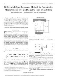
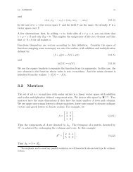
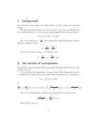
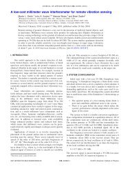
104 CHAPTER 4. FOURIER ANALYSIS4.2 The Fourier SeriesSo, the motivation for further study of such a Fourier superposition is clear. But thereare other important reasons as well. For instance, consider the data shown in Figure 4.1.These are borehole tiltmeter measurements. A tiltmeter is a device that measures thelocal tilt relative to the earth’s gravitational field. The range of tilts shown here isbetween -40 and 40 nanoradians! (There are 2 π radians in 360 degrees, so this rangecorresponds to about 8 millionths of a degree.) With this sensitivity, you would expectthat the dominant signal would be due to earth tides. So buried in the time-series on thetop you would expect to see two dominant frequencies, one that was diurnal (1 cycle perday) and one that was semi-diurnal (2 cycles per day). If we somehow had an automaticway of representing these data as a superposition of sinusoids of various frequencies,then might we not expect these characteristic frequencies to manifest themselves inthe size of the coefficients of this superposition? The answer is yes, and this is one ofthe principle aims of Fourier analysis. In fact, the power present in the data at eachfrequency is called the power spectrum. Later we will see how to estimate the powerspectrum using a Fourier transform.You’ll notice in the tiltmeter spectrum that the two peaks (diurnal and semi-diurnalseem to be split; i.e., there are actually two peaks centered on 1 cycle/day and twopeaks centered on 2 cycles/day. Consider the superposition of two sinusoids of nearlythe same frequency:sin((ω − ɛ)t) + sin((ω + ɛ)t).Show that this is equal to2 cos(ɛt) sin(ωt).Interpret this result physically, keeping in mind that the way we’ve set the problemup, ɛ is a small number compared to ω. It might help to make some plots. Onceyou’ve figured out the interpretation of this last equation, do you see evidence of thesame effect in the tiltmeter data?There is also a drift in the tiltmeter. Instead of the tides fluctuating about 0 tilt, theyslowly drift upwards over the course of 50 days. This is likely a drift in the instrumentand not associated with any tidal effect. Think of how you might correct the data forthis drift.As another example Figure 4.2 shows 50 milliseconds of sound (a low C) made by asoprano saxophone and recorded on a digital oscilloscope. Next to this is the estimatedpower spectrum of the same sound. Notice that the peaks in the power occur at integermultiples of the frequency of the first peak (the nominal frequency of a low C).

4.2. THE FOURIER SERIES 10540Measured Borehole TiltTilt (nradians)200−20Power Spectral Density (dB/Hz)−400 5 10 15 20 25 30 35 40 45 50time (days)500MTM PSD Estimate−500 0.5 1 1.5 2 2.5 3 3.5 4 4.5 5Frequency (cycles/day)Figure 4.1: Borehole tiltmeter measurements. Data courtesy of Dr. Judah Levine (see[6] for more details). The plot on the top shows a 50 day time series of measurements.The figure on the bottom shows the estimated power in the data at each frequencyover some range of frequencies. This is known as an estimate of the power spectrumof the data. Later we will learn how to compute estimates of the power spectrum oftime series using the Fourier transform. Given what we know about the physics of tilt,we should expect that the diurnal tide (once per day) should peak at 1 cycle per day,while the semi-diurnal tide (twice per day) should peak at 2 cycles per day. This sortof analysis is one of the central goals of Fourier theory.

106 CHAPTER 4. FOURIER ANALYSISLow C on soprano saxophoneLow C on soprano saxophone−20−40Power (db)−60−800.000 0.010 0.020 0.030 0.040 0.050Time (sec)−1000 1000 2000 3000 4000 5000 6000Frequency (Hz)Figure 4.2: On the left is .05 seconds of someone playing low C on a soprano saxophone.On the right is the power spectrum of these data. We’ll discuss later how this computationis made, but essentially what you’re seeing the power as a function of frequency.The first peak on the right occurs at the nominal frequency of low C. Notice that allthe higher peaks occur at integer multiples of the frequency of the first (fundamental)peak.Definition of the Fourier SeriesFor a function periodic on the interval [−l, l], the Fourier series is defined to be:or equivalently,f(x) = a 02 + ∞ ∑n=1f(x) =a n cos(nπx/l) + b n sin(nπx/l). (4.1)∞∑n=−∞c n e inπx/l . (4.2)We will see shortly how to compute these coefficients. The connection between the realand complex coefficients is:c k = 1 2 (a k − ib k ) c −k = 1 2 (a k + ib k ). (4.3)In particular notice that the sine/cosine series has only positive frequencies, while theexponential series has both positive and negative. The reason is that in the former caseeach frequency has two functions associated with it. If we introduce a single complexfunction (the exponential) we avoid this by using negative frequencies. In other words,any physical vibration always involves two frequencies, one positive and one negative.Later on you will be given two of the basic convergence theorems for Fourier series.Now let’s look at some examples.

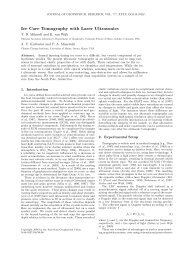
4.2. THE FOURIER SERIES 10710.80.60.40.24.2.1 Examples-1 -0.5 0.5 1Figure 4.3: Absolute value function.Let f(x) = abs(x), as shown in Figure 4.3. The first few terms of the Fourier series are:1 4 cos(π x) 4 cos(3 π x) 4 cos(5 π x)− − − (4.4)2 π 2 9 π 2 25 π 2This approximation is plotted in Figure 4.3.ObservationsNote well that the convergence is slowest at the origin, where the absolute value functionis not differentiable. (At the origin, the slope changes abruptly from -1 to +1. So theleft derivative and the right derivative both exist, but they are not the same.) Also, asfor any even function (i.e., f(x) = f(−x)) only the cosine terms of the Fourier seriesare nonzero.Suppose now we consider an odd function (i.e., f(x) = −f(−x)), such as f(x) = x.The first four terms of the Fourier series are2 sin(π x)π−sin(2 π x)π+2 sin(3 π x)3 π−sin(4 π x)2 π(4.5)Here you can see that only the sine terms appear, and no constant (zero-frequency)term. A plot of this approximation is shown in Figure 4.5.So why the odd behavior at the endpoints? It’s because we’ve assume the function isperiodic on the interval [−1, 1]. The periodic extension of f(x) = x must therefore have

108 CHAPTER 4. FOURIER ANALYSIS0.80.60.40.2-1 -0.5 0.5 1Figure 4.4: First four nonzero terms of the Fourier series of the function f(x) = abs(x).10.5-1 -0.5 0.5 1-0.5-1Figure 4.5: First four nonzero terms of the Fourier series of the function f(x) = x.

4.3. SUPERPOSITION AND ORTHOGONAL PROJECTION 10910.80.60.40.20.5 1 1.5 2 2.5 3Figure 4.6: Periodic extension of the function f(x) = x relative to the interval [0, 1].a sort of sawtooth appearance. In other words any non-periodic function defined on afinite interval can be used to generate a periodic function just by cloning the functionover and over again. Figure 4.6 shows the periodic extension of the function f(x) = xrelative to the interval [0, 1]. It’s a potentially confusing fact that the same functionwill give rise to different periodic extensions on different intervals. What would theperiodic extension of f(x) = x look like relative to the interval [−.5, .5]?4.3 Superposition and orthogonal projectionNow, recall that for any set of N linearly independent vectors x i in R N , we can representan arbitrary vector z in R N as a superpositionwhich is equivalent to the linear systemz = c 1 x 1 + c 2 x 2 + · · · + c N x N , (4.6)z = X · c (4.7)where X is the matrix whose columns are the x i vectors and c is the vector of unknownexpansion coefficients. As you well know, matrix equation has a unique solution c ifand only if the x i are linearly independent. But the solution is especially simple if thex i are orthogonal. Suppose we are trying to find the coefficients ofz = c 1 q 1 + c 2 q 2 + · · · + q N , (4.8)when q i · q j = δ ij . In this case we can find the coefficients easily by projecting onto theorthogonal directions:c i = q i · z, (4.9)

110 CHAPTER 4. FOURIER ANALYSISor, in the more general case where the q vectors are orthogonal but not necessarilynormalizedc i = q i · zq i · q i. (4.10)We have emphasized throughout this course that functions are vectors too, they justhappen to live in an infinite dimensional vector space (for instance, the space of squareintegrable functions). So it should come as no surprise that we would want to considera formula just like 4.8, but with functions instead of finite dimensional vectors; e.g.,f(x) = c 1 q 1 (x) + c 2 q 2 (x) + · · · + c n q n (x) + · · · . (4.11)In general, the sum will require an infinite number of coefficients c i , since a functionhas an infinite amount of information. (Think of representing f(x) by its value at eachpoint x in some interval.) Equation 4.11 is nothing other than a Fourier series if theq(x) happen to be sinusoids. Of course, you can easily think of functions for whichall but a finite number of the coefficients will be zero; for instance, the sum of a finitenumber of sinusoids.Now you know exactly what is coming. If the basis functions q i (x) are “orthogonal”,then we should be able to compute the Fourier coefficients by simply projecting thefunction f(x) onto each of the orthogonal “vectors” q i (x). So, let us define a dot (orinner) product for functions on an interval [−l, l] (this could be an infinite interval)(u, v) ≡∫ l−lu(x)v(x)dx. (4.12)Then we will say that two functions are orthogonal if their inner product is zero.Now we simply need to show that the sines and cosines (or complex exponentials) areorthogonal. Here is the theorem. Let φ k (x) = sin(kπx/l) and ψ k (x) = cos(kπx/l).Then(φ i , φ j ) = (ψ i , ψ j ) = lδ ij (4.13)(φ i , ψ j ) = 0. (4.14)The proof, which is left as an exercise, makes use of the addition formulae for sines andcosines. (If you get stuck, the proof can be found in [2], Chapter 10.) A similar resultholds for the complex exponential, where we define the basis functions as ξ k (x) = e ikπx/l .Using Equations 4.13 and 4.14 we can compute the Fourier coefficients by simply projectingf(x) onto each orthogonal basis vector:anda n = 1 l∫ l−l∫ lf(x) cos(nπx/l)dx = 1 l (f, ψ n), (4.15)b n = 1 f(x) sin(nπx/l)dx = 1 l −ll (f, φ n). (4.16)Or, in terms of complex exponentialsc n = 1 2l∫ l−lf(x)e −inπx/l dx. (4.17)

4.4. THE FOURIER INTEGRAL 1114.4 The Fourier IntegralFor a function defined on any finite interval, we can use the Fourier series, as above.For functions that are periodic on some other interval than [−l, l] all we have to doto use the above formulae is to make a linear change of variables so that in the newcoordinate the function is defined on [−l, l]. And for functions that are not periodic atall, but still defined on a finite interval, we can fake the periodicity by replicating thefunction over and over again. This is called periodic extension.OK, so we have a function that is periodic on an interval [−l, l]. Looking at its Fourierseries (either Equation 4.1 or 4.2) we see straight away that the frequencies present inthe Fourier synthesis aref 1 = 1 2l , f 2 = 2 2l , f 3 = 3 2l , · · · , f k = k 2l · · · (4.18)Suppose we were to increase the range of the function to a larger interval [−L, L] triviallyby defining it to be zero on [−L, −l] and [l, L]. To keep the argument simple, let ussuppose that L = 2l. Then we notice two things straight away. First, the frequenciesappearing in the Fourier synthesis are nowf 1 = 12L , f 2 = 22L , f 3 = 32L , · · · , f k = k2L · · · (4.19)So the frequency interval is half what it was before. And secondly, we notice that half ofthe Fourier coefficients are the same as before, with the new coefficients appearing midwaybetween the old ones. Imagine continuing this process indefinitely. The Fouriercoefficients become more and more densely distributed, until, in the limit that L → ∞,the coefficient sequence c n becomes a continuous function. We call this function theFourier transform of f(x) and denote it by F (k). In this case, our Fourier seriesbecomesf(x) =∞∑n=−∞f(x) = 1 √2π∫ ∞−∞c n e inπx/lF (k)e ikx dk (4.20)with the “coefficient” function F (k) being determined, once again, by orthogonal projection:F (k) = √ 1 ∫ ∞f(x)e −ikx dx (4.21)2π−∞NormalizationA function f(t) is related to its Fourier transform f(ω) via:f(t) = 1 √2π∫ ∞−∞F (ω)e iωt dω (4.22)

112 CHAPTER 4. FOURIER ANALYSISandF (ω) = 1 √2π∫ ∞−∞f(t)e −iωt dt (4.23)It doesn’t matter how we split up the 2π normalization. For example, in the interest ofsymmetry we have defined both the forward and inverse transform with a 1/ √ 2π outfront. Another common normalization isandf(t) = 1 ∫ ∞F (ω)e iωt dω (4.24)2π −∞F (ω) =∫ ∞−∞f(t)e −iωt dt. (4.25)It doesn’t matter how we do this as long as we’re consistent. We could get rid of thenormalization altogether if we stop using circular frequencies ω in favor of f measuredin hertz or cycles per second. Then we haveg(t) =∫ ∞−∞G(f)e 2πift df (4.26)andG(f) =∫ ∞−∞g(t)e −2πift dt (4.27)Here, using time and frequency as variables, we are thinking in terms of time series,but we could just as well use a distance coordinate such as x and a wavenumber k:with the inverse transformation beingf(x) = 1 ∫ ∞F (k)e ikx dk (4.28)2π −∞F (k) =∫ ∞−∞f(x)e −ikx dx. (4.29)Invertibility: the Dirichlet KernelThese transformations from time to frequency or space to wavenumber are invertiblein the sense that if we apply one after the other we recover the original function. Tosee this plug Equation (4.29) into Equation (4.28):f(x) = 1 ∫ ∞2π −∞∫ ∞dk f(x ′ )e −ik(x′ −x) dx ′ . (4.30)−∞If we define the kernel function K(x − x ′ , µ) such thatK(x ′ − x, µ) = 1 ∫ µe −ik(x′ −x) dk = sin µ(x′ − x)2π −µπ(x ′ − x)(4.31)

114 CHAPTER 4. FOURIER ANALYSIS330220110-1 -0.5 0.5 1-1 -0.5 0.5 110 10030025020015010050-1 -0.5 0.5 1-50100030002500200015001000500-1 -0.5 0.5 110000Figure 4.7: The kernel sin µx/πx for µ = 10, 100, 1000, and 10000.This function is shown in Figure 4.8 and is just the Dirichlet kernel for µ = 1, centeredabout the origin. 1Here is a result which is a special case of a more general theorem telling us how theFourier transform scales. Let f(x) = e −x2 /a 2 . Here a is a parameter which correspondsto the width of the bell-shaped curve. Make a plot of this curve. When a is small, thecurve is relatively sharply peaked. When a is large, the curve is broadly peaked. Nowcompute the Fourier transform of f:F (k) ∝∫ ∞−∞e −x2 /a 2 e −ikx dx.The trick to doing integrals of this form is to complete the square on the exponentials.You want to write the whole thing as an integral of the form∫ ∞e −z2 dz.−∞As you’ll see shortly, this integral can be done analytically. The details will be left asan exercise, here we will just focus on the essential feature, the exponential.So the integral reduces toe −x2 /a 2 e −ikx = e −1/a2 [(x+ika 2 /2) 2 +(ka 2 /2) 2 ] .∫ ∞ae −k2 a 2 /4−∞e −z2 dz = √ πae −k2 a 2 /4 .1 To evaluate the limit of this function at k = 0, use L’Hôpital’s rule.

4.4. THE FOURIER INTEGRAL 11521.510.5-10 -5 5 10Figure 4.8: The Fourier transform of the box function.(The √ π will come next.) So we see that in the Fourier domain the factor of a 2 appearsin the numerator of the exponential, whereas in the original domain, it appeared inthe denominator. Thus, making the function more peaked in the space/time domainmakes the Fourier transform more broad; while making the function more broad inthe space/time domain, makes it more peaked in the Fourier domain. This is a veryimportant idea.Now the trick to doing the Gaussian integral. SinceThereforeSo H = √ π.[∫ ∞H 2 =H 2 =e −x2−∞∫ ∞ ∫ 2π00H =] [∫ ∞dx e −y2−∞∫ ∞e −x2−∞e −r2 r dr dθ = 1 2dx] ∫ ∞ ∫ ∞dy = e −(x2 +y 2) dx dy.−∞ −∞∫ ∞ ∫ 2π00e −ρ dρ dθ = π4.4.2 Some Basic Theorems for the Fourier TransformIt is very useful to be able think of the Fourier transform as an operator acting onfunctions. Let us define an operator Φ viaΦ[f] = F (4.33)whereF (ω) =∫ ∞−∞f(t)e −iωt dt. (4.34)

116 CHAPTER 4. FOURIER ANALYSISThen it is easy to see that Φ is a linear operatorNext, if f (k) denotes the k-th derivative of f, thenΦ[c 1 f 1 + c 2 f 2 ] = c 1 Φ[f 1 ] + c 2 Φ[f 2 ]. (4.35)Φ[f (k) ] = (iω) k Φ[f] k = 1, 2, . . . (4.36)This result is crucial in using Fourier analysis to study differential equations. Next,suppose c is a real constant, thenandΦ[f(t − c)] = e −icw Φ[f] (4.37)Φ[e ict f(t)] = F (t − c) (4.38)where F = Φ(f). And finally, we have the convolution theorem. For any two functionsf(t) and g(t) with F = Φ(f) and G = Φ(g), we havewhere “*” denotes convolution:[f ∗ g](t) =Φ(f)Φ(g) = Φ[f ∗ g] (4.39)∫ ∞−∞f(τ)g(t − τ)dτ. (4.40)The convolution theorem is one of the most important in time series analysis. Convolutionsare done often and by going to the frequency domain we can take advantage ofthe algorithmic improvements of the fast Fourier transform algorithm (FFT).The proofs of all these but the last will be left as an exercise. The convolution theoremis worth proving. Start by multiplying the two Fourier transforms. We will throwcaution to the wind and freely exchange the orders of integration. Also, let’s ignore thenormalization for the moment:∫ ∞∫ ∞F (ω)G(ω) = f(t)e −iωt dt g(t ′ )e −iωt′ dt ′ (4.41)===−∞∫ ∞ ∫ ∞−∞ −∞∫ ∞ ∫ ∞−∞ −∞∫ ∞ [∫ ∞e −iωτ−∞−∞−∞e −iω(t+t′) f(t)g(t ′ )dt dt ′ (4.42)e −iωτ f(t)g(τ − t)dt dτ (4.43)]f(t)g(τ − t)dt dτ. (4.44)This completes the proof, but now what about the normalization? If we put the symmetric1/ √ 2π normalization in front of both transforms, we end up with a left-overfactor of 1/ √ 2π because we started out with two Fourier transforms and we ended upwith only one and a convolution. On the other hand, if we had used an asymmetricnormalization, then the result would be different depending on whether we put the1/(2π) on the forward or inverse transform. This is a fundamental ambiguity since wecan divide up the normalization anyway we want as long as the net effect is 1/(2π).This probably the best argument for using f instead of ω since then the 2πs are in theexponent and the problem goes away.

4.5. THE SAMPLING THEOREM 1174.5 The Sampling TheoremNow returning to the Fourier transform, suppose the spectrum of our time series f(t) iszero outside of some symmetric interval [−2πf s , 2πf s ] about the origin. 2 In other words,the signal does not contain any frequencies higher than f s hertz. Such a function issaid to be band limited; it contains frequencies only in the band [−2πf s , 2πf s ]. Clearlya band limited function has a finite inverse Fourier transformf(t) = 12π∫ 2πfs−2πf sF (ω)e −iωt dω. (4.45)sampling frequencies and periodsf s is called the sampling frequency. Hence the sampling period is T s ≡ 1/f s . It issometimes convenient to normalize frequencies by the sampling frequency. Then themaximum normalized frequency is 1:ˆf = ˆω 2π = fT s = f/f s .Since we are now dealing with a function on a finite interval we can represent it as aFourier series:∞∑F (ω) = φ n e iωn/2fs (4.46)n=−∞where the Fourier coefficients φ n are to be determined byφ n = 14πf s∫ 2πfs−2πf sF (ω)e −iωn/2fs dω. (4.47)Comparing this result with our previous work we can see thatφ n = f(n/2f s)2f s(4.48)where f(n/2f s ) are the samples of the original continuous time series f(t). Putting allthis together, one can show that the band limited function f(t) is completely specifiedby its values at the countable set of points spaced 1/2f s apart:f(t) =14πf s∞ ∑n=−∞∫ 2πfsf(n/2f s ) e i(ωn/2fs−ωt) dω−2πf s2 In fact the assumption that the interval is symmetric about the origin is made without loss ofgenerality, since we can always introduce a change of variables which maps an arbitrary interval intoa symmetric one centered on 0.

118 CHAPTER 4. FOURIER ANALYSIS=∞∑n=−∞f(n/2f s ) sin(π(2f st − n)). (4.49)π(2f s t − n)The last equation is known as the Sampling Theorem. Notice that the functionsin x/x appears here too. Since this function appears frequently it is given a specialname, it is called the sinc function:sinc(x) = sinxx .And we know that the sinc function is also the Fourier transform of a box-shapedfunction. So the sampling theorem says take the value of the function, sampled every1/2f s , multiply it by a sinc function centered on that point, and then sum these up forall the samples.It is worth repeating for emphasis: any band limited function is completely determinedby its samples chosen 1/2f s apart, where f s is the maximum frequency contained inthe signal. This means that in particular, a time series of finite duration (i.e., any realtime series) is completely specified by a finite number of samples. It also means that ina sense, the information content of a band limited signal is infinitely smaller than thatof a general continuous function. So if our band-limited signal f(t) has a maximumfrequency of f s hertz, and the length of the signal is T , then the total number of samplesrequired to describe f is 2f s T .A sampling exerciseConsider the continuous sinusoidal signal:x(t) = A cos(2πft + φ)Suppose we sample this signal at a sampling period of T s . Let us denote the discretesamples of the signal with square brackets:x[n] ≡ x(nT s ) = A cos(2πfnT s + φ).Now consider a different sinusoid of the same amplitude and phase, but sampled at afrequency of f +lf s , where l is an integer and f s = 1/T s . Let the samples of this secondsinusoid be denoted by y[n]. Show that x[n] = y[n]. This is an example of aliasing.These two sinusoids have exactly the same samples, so the frequency of one appears tobe the same.

4.5. THE SAMPLING THEOREM 119The sampling theorem is due to Harry Nyquist, a researcher at Bell Labs in NewJersey. In a 1928 paper Nyquist laid the foundations for the sampling of continuoussignals and set forth the sampling theorem. Nyquist was born on February 7, 1889in Nilsby, Sweden and emigrated to the US in 1907. He got his PhD in Physics fromYale in 1917. Much of Nyquist’s work in the 1920’s was inspired by the telegraph. Inaddition to his work in sampling, Nyquist also made an important theoretical analysisof thermal noise in electrical systems. In fact this sort of noise is sometimes calledNyquist noise. Nyquist died on April 4, 1976 in Harlingen, Texas.A generation after Nyquist’s pioneering work Claude Shannon, alsoat Bell Labs, laid the broad foundations of modern communicationtheory and signal processing. Shannon (Born: April 1916 in Gaylord,Michigan; Died: Feb 2001 in Medford, Massachusetts) was the founderof modern information theory. After beginning his studies in electricalengineering, Shannon took his PhD in mathematics from MIT in 1940.Shannon’s A Mathematical Theory of Communication published in1948 in the Bell System Technical Journal, is one of the profoundly influential scientificworks of the 20th century. In it he introduced many ideas that became the basis forelectronic communication, such as breaking down information into sequences of 0’sand 1’s (this is where the term bit first appeared), adding extra bits to automaticallycorrect for errors and measuring the information or variability of signals. Shannon’spaper and many other influential papers on communication are compiled in the bookKey papers in the development of information theory [7].4.5.1 AliasingAs we have seen, if a time-dependent function contains frequencies up to f s hertz, thendiscrete samples taken at an interval of 1/2f s seconds completely determine the signal.Looked at from another point of view, for any sampling interval ∆, there is a specialfrequency (called the Nyquist frequency), given by f s = 1 . The extrema (peaks and2∆troughs) of a sinusoid of frequency f s will lie exactly 1/2f s apart. This is equivalent tosaying that critical sampling of a sine wave is 2 samples per wavelength.We can sample at a finer interval without introducing any error; the samples will beredundant, of course. However, if we sample at a coarser interval a very serious kindof error is introduced called aliasing. Figure 4.9 shows a cosine function sampled at aninterval longer than 1/2f s ; this sampling produces an apparent frequency of 1/3 thetrue frequency. This means that any frequency component in the signal lying outsidethe interval (−f s , f s ) will be spuriously shifted into this interval. Aliasing is producedby under-sampling the data: once that happens there is little that can be done to

120 CHAPTER 4. FOURIER ANALYSIS10.51 2 3 4-0.5-1Figure 4.9: A sinusoid sampled at less than the Nyquist frequency gives rise to spuriousperiodicities.correct the problem. The way to prevent aliasing is to know the true band-width ofthe signal (or band-limit the signal by analog filtering) and then sample appropriatelyso as to give at least 2 samples per cycle at the highest frequency present.4.6 The Discrete Fourier TransformNow we consider the third major use of the Fourier superposition. Suppose we have discretedata, not a continuous function. In particular, suppose we have data f k recordedat locations x k . To keep life simple, let us suppose that the data are recorded at Nevenly spaced locations x k = 2πk/N, k = 0, 1, . . . N − 1. Think of f k as being samplesof an unknown function, which we want to approximate. Now we write down a Fourierapproximation for the unknown function (i.e., a Fourier series with coefficients to bedetermined):p(x) =N−1 ∑n=0c n e inx . (4.50)Now we will compute the coefficients in such a way that p interpolates (i.e., fits exactly)the data at each x k :f k = p(x k ) =N−1 ∑n=0c n e in2πk/N . (4.51)In theory we could do this for any linearly independent set of basis functions by solvinga linear system of equations for the coefficients. But since sines/cosines are orthogonal,the c n coefficients can be computed directly:c k = 1 NN−1 ∑n=0f n e −in2πk/N . (4.52)

4.7. THE LINEAR ALGEBRA OF THE DFT 121This is the discrete version of the Fourier transform (DFT). f n are the data and c k arethe harmonic coefficients of a trigonometric function that interpolates the data. Now,of course, there are many ways to interpolate data, but it is a theorem that the onlyway to interpolate with powers of e i2πx is Equation 4.52.Optional Exercise In the handout you will see some Mathematica code for computingand displaying discrete Fourier transforms. Implement the previous formula andcompare the results with Mathematica’s built in Fourier function. You should get thesame result, but it will take dramatically longer than Mathematica would for 100 datapoints. The reason is that Mathematica uses a special algorithm called the FFT (FastFourier Transform). See Strang for an extremely clear derivation of the FFT algorithm.4.7 The Linear Algebra of the DFTTake a close look at Equation 4.52. Think of the DFT coefficients c k and the datapoints f n as being elements of vectors c and f. There are N coefficients and N dataso both c and f are elements of R N . The summation in the Fourier interpolation istherefore a matrix-vector inner product. Let’s identify the coefficients of the matrix.Define a matrix Q such thatQ nk = e in2πk/N . (4.53)N is fixed, that’s just the number of data points. The matrix appearing in Equation4.52 is the complex conjugate of Q; i.e., Q ∗ . We can write Equation 4.51 asf = Q · c. (4.54)The matrix Q is almost orthogonal. We have said that a matrix A is orthogonal ifAA T = A T A = I, where I is the N-dimensional identity matrix. For complex matriceswe need to generalize this definition slightly; for complex matrices we will say that Ais orthogonal if (A T ) ∗ A = A(A T ) ∗ = I. 3 In our case, since Q is obviously symmetric,we have:Q ∗ Q = QQ ∗ = I. (4.55)Once again, orthogonality saves us from having to solve a linear system of equations:since Q ∗ = Q −1 , we havec = Q ∗ · f. (4.56)Now you may well ask: what happens if we use fewer Fourier coefficients than we havedata? That corresponds to having fewer unknowns (the coefficients) than data. Soyou wouldn’t expect there to be an exact solution as we found with the DFT, but howabout a least squares solution? Let’s try getting an approximation function of the form3 Technically such a matrix is called Hermitian or self-adjoint–the operation of taking the complexconjugate transpose being known at the adjoint–but we needn’t bother with this distinction here.

122 CHAPTER 4. FOURIER ANALYSISm∑p(x) = c n e inx (4.57)where now we sum only up to m < N − 1. Our N equations in m unknowns is now:n=0m∑f k = c n e in2πk/N . (4.58)n=0So to minimize the mean square error we set the derivative of||f − Q · c|| 2 (4.59)with respect to an arbitrary coefficient, say c j , equal to zero. But this is just an ordinaryleast squares problem.4.8 The DFT from the Fourier IntegralIn this section we will use the f (cycles per second) notation rather than the ω (radiansper second), because there are slightly fewer factors of 2π floating around. You should becomfortable with both styles, but mind those 2πs! Also, up to now, we have avoided anyspecial notation for the Fourier transform of a function, simply observing whether it wasa function of space-time or wavenumber-frequency. Now that we are considering discretetransforms and real data, we need to make this distinction since we will generally haveboth the sampled data and its transform stored in arrays on the computer. So for thissection we will follow the convention that if h = h(t) then H = H(f) is its Fouriertransform.We suppose that our data are samples of a function and that the samples are taken atequal intervals, so that we can writeh k ≡ h(t k ), t k ≡ k∆, k = 0, 1, 2, . . . , N − 1, (4.60)where N is an even number. In our case, the underlying function h(t) is unknown; allwe have are the digitally recorded time series. But in either case we can estimate theFourier transform H(f) at at most N discrete points chosen in the range −f s to f swhere f s is the Nyquist frequency: 4f n ≡n∆N , n = −N 2 , . . . , N 2 . (4.61)The two extreme values of frequency f −N/2 and f −N/2 are not independent (f −N/2 =−f N/2 ), so there are actually only N independent frequencies specified above.4 The highest frequency f s in the Fourier representation of a time series sampled at a time interval1of ∆ is2∆. This maximum frequency is called the Nyquist frequency. You’ll study this in detail inthe digital course.

4.8. THE DFT FROM THE FOURIER INTEGRAL 123A sensible numerical approximation for the Fourier transform integral is thus:H(f n ) =∫ ∞−∞h(t)e −2πifnt dt ≈N−1 ∑k=0h k e −2πifnt k∆. (4.62)ThereforeN−1 ∑H(f n ) ≈ ∆ h k e −2πikn/N . (4.63)k=0Defining the Discrete Fourier Transform (DFT) bywe then haveH n =where f n are given by Equation (4.61).N−1 ∑k=0h k e −2πikn/N (4.64)H(f n ) ≈ ∆H n (4.65)Now, the numbering convention implied by Equation (4.61) has ± Nyquist at the extremeends of the range and zero frequency in the middle. However it is clear that theDFT is periodic with period N:H −n = H N−n . (4.66)As a result, it is standard practice to let the index n in H n vary from 0 to N − 1,with n and k varying over the same range. In this convention 0 frequency occurs atn = 0; positive frequencies from from 1 ≤ n ≤ N/2 − 1; negative frequencies run fromN/2 + 1 ≤ n ≤ N − 1. Nyquist sits in the middle at n = N/2. The inverse transformis:h k = 1 NN−1 ∑n=0H n e 2πikn/N (4.67)Mathematica, on the other hand, uses different conventions. It uses the symmetricnormalization (1/ √ N in front of both the forward and inverse transform), and definesarrays running from 1 to N in Fortran fashion. So in Mathematica, the forward andinverse transforms are, respectively:andH n = √ 1 ∑ N h k e −2πi(k−1)(n−1)/N (4.68)Nk=1h k = 1 √N N ∑n=1H n e 2πi(k−1)(n−1)/N . (4.69)If you are using canned software, make sure you know what conventions arebeing used.

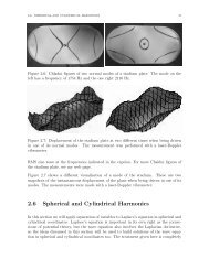
124 CHAPTER 4. FOURIER ANALYSIS0.60.40.2-0.2-0.410 20 30 40 50 600.40.2-0.2-0.410 20 30 40 50 600.10.10.050.05-0.0510 20 30 40 50 60-0.0510 20 30 40 50 60-0.1-0.10.10.10.050.05-0.0510 20 30 40 50 60-0.0510 20 30 40 50 60-0.1-0.1Figure 4.10: The real (left) and imaginary (right) parts of three length 64 time series,each associated with a Kronecker delta frequency spectrum. These time series arereconstructed from the spectra by inverse DFT. At the top the input spectrum is δ i,0 ,in the middle δ i,1 , and at the bottom, δ i,64/2−1 .4.8.1 Discrete Fourier Transform ExamplesHere we show a few examples of the use of the DFT. What we will do is construct anunknown time series’ DFT by hand and inverse transform to see what the resultingtime series looks like. In all cases the time series h k is 64 samples long. Figures 4.10and 4.11 show the real (left) and imaginary (right) parts of six time series that resultedfrom inverse DFT’ing an array H n which was zero except at a single point (i.e., it’s aKronecker delta: H i = δ i,j = 1 if i = j and zero otherwise; here a different j is chosenfor each plot). Starting from the top and working down, we choose j to be the followingsamples: the first, the second, Nyquist-1, Nyquist, Nyquist+1, the last. We can seethat the first sample in frequency domain is associated with the zero-frequency or DCcomponent of a signal and that the frequency increases until we reach Nyquist, whichis in the middle of the array. Next, in Figure 4.12, we show at the top an input timeseries consisting of a pure sinusoid (left) and the real part of its DFT. Next we addsome random noise to this signal. On the left in the middle plot is the real part of thenoisy signals DFT. Finally, at the bottom, we show a Gaussian which we convolve withthe noisy signal in order to attenuate the frequency components in the signal. The realpart of the inverse DFT of this convolved signal is shown in the lower right plot.

4.8. THE DFT FROM THE FOURIER INTEGRAL 1250.10.050.40.210 20 30 40 50 6010 20 30 40 50 60-0.05-0.1-0.2-0.40.10.050.10.0510 20 30 40 50 6010 20 30 40 50 60-0.05-0.1-0.05-0.10.10.050.10.0510 20 30 40 50 6010 20 30 40 50 60-0.05-0.1-0.05-0.1Figure 4.11: The real (left) and imaginary (right) parts of three time series of length64, each associated with a Kronecker delta frequency spectrum. These time series arereconstructed from the spectra by inverse DFT. At the top the input spectrum is δ i,64/2 ,in the middle δ i,64/2+1 , and at the bottom δ i,64 .

126 CHAPTER 4. FOURIER ANALYSIS10.5-0.510 20 30 40 50 601.51.2510.750.50.25-110 20 30 40 50 601.510.54310 20 30 40 50 602-0.5-1110 20 30 40 50 600.80.60.40.20.410 20 30 40 50 600.2-0.210 20 30 40 50 60-0.4Figure 4.12: The top left plot shows an input time series consisting of a single sinusoid.In the top right we see the real part of its DFT. Note well the wrap-around at negativefrequencies. In the middle we show the same input sinusoid contaminated with someuniformly distributed pseudo-random noise and its DFT. At the bottom left, we showa Gaussian time series that we will use to smooth the noisy time series by convolvingit with the DFT of the noisy signal. When we inverse DFT to get back into the “time”domain we get the smoothed signal shown in the lower right.

4.9. CONVERGENCE THEOREMS 1274.9 Convergence TheoremsOne has to be a little careful about saying that a particular function is equal to itsFourier series since there exist piecewise continuous functions whose Fourier series divergeeverywhere! However, here are two basic results about the convergence of suchseries.Point-wise Convergence Theorem: If f is piecewise continuous and has left andright derivatives at a point c 5 then the Fourier series for f converges converges to1(f(c−) + f(c+)) (4.70)2where the + and - denote the limits when approached from greater than or less than c.Another basic result is the Uniform Convergence Theorem: If f is continuouswith period 2π and f ′ is piecewise continuous, then the Fourier series for f convergesuniformly to f. For more details, consult a book on analysis such as The Elements ofReal Analysis by Bartle [1] or Real Analysis by Haaser and Sullivan [4].4.10 Basic Properties of Delta FunctionsAnother representation of the delta function is in terms of Gaussian functions:δ(x) = lim µ→∞µ √π e −µ2 x 2 . (4.71)You can verify for yourself that the area under any of the Gaussian curves associatedwith finite µ is one.The spectrum of a delta function is completely flat since∫ ∞e −ikx δ(x) dx = 1. (4.72)−∞For delta functions in higher dimensions we need to add an extra 1/2π normalizationfor each dimension. Thusδ(x, y, z) =( ) 1 3 ∫ ∞ ∫ ∞ ∫ ∞e i(kxx+kyy+kzz) dk x dk y dk z . (4.73)2π −∞ −∞ −∞The other main properties of delta functions are the following:δ(x) = δ(−x) (4.74)5 A right derivative would be: lim t→0 (f(c + t) − f(c))/t, t > 0. Similarly for a left derivative.

128 CHAPTER 4. FOURIER ANALYSIS∫∫δ(ax) = 1 δ(x) (4.75)|a|xδ(x) = 0 (4.76)f(x)δ(x − a) = f(a)δ(x − a) (4.77)δ(x − y)δ(y − a) dy = δ(x − a) (4.78)∫ ∞δ (m) f(x) dx = (−1) m f (m) (0) (4.79)−∞δ ′ (x − y)δ(y − a) dy = δ ′ (x − a) (4.80)xδ ′ (x) = −δ(x) (4.81)δ(x) = 1 ∫ ∞e ikx dk (4.82)2π −∞δ ′ (x) = i ∫ ∞ke ikx dk (4.83)2π −∞• Prove Equations 4.4 and 4.5.Exercises• Compute the Fourier transform of the following function. f(x) is equal to 0 forx < 0, x for 0 ≤ x ≤ 1 and 0 for x > 1.• Prove Equations 4.35, 4.36, 4.37, 4.39.• Compute the Fourier transform of f(x) = e −x2 /a 2 . If a is small, this bell-shapedcurve is sharply peaked about the origin. If a is large, it is broad. What can yousay about the Fourier transform of f in these two cases?• Let f(x) be the function which is equal to -1 for x < 0 and +1 for x > 0. Assumingthatf(x) = a 0∞2 + ∑∞∑a k cos(kπx/l) + b k sin(kπx/l),k=1compute a 0 , a 1 , a 2 , b 1 and b 2 by hand, taking the interval of periodicity to be[−1, 1].• For an odd function, only the sine or cosine terms appear in the Fourier series.Which is it?• Consider the complex exponential form of the Fourier series of a real function∞∑f(x) = c n e inπx/l .n=−∞Take the complex conjugate of both sides. Then use the fact that since f is real,it equals its complex conjugate. What does this tell you about the coefficients c n ?k=1