Evaluation of Differential and Common - Mode Transmission ...

Evaluation of Differential and Common - Mode Transmission Through UTPCables Using FE TechniquesS. Dorai 1 , W. Yin 1 , J. Kelly 2 and A. J. Peyton 11School of Electrical and Electronic Engineering, The University of Manchester, Manchester, M60 1QD2 Middlegate, White Lund Industrial Estate, Morecambe, LA3 3BN, U.K+44-161-306-2870 · Sriram.dorai@postgrad.manchester.ac.ukAbstractThe purpose of this paper is to demonstrate a methodology forpredicting the amount of energy propagating differentially and incommon mode for a UTP (Unshielded twisted pair) cable using FE(Finite element) techniques. Several cases are considered, such as aproperly terminated line with no source or load impedancemismatch and other combinations of improperly terminated lines.Consequently, the relative signal strength of the differential andcommon mode components of the transmitted and reflected signalscan be determined in the form of voltage versus distance versus timematrix, which is plotted to show the full evolution of energy transferalong the cable versus time.Keywords: Differential and common mode signals, UTP cables,Finite element techniques, wall and patch panel connectors.1. IntroductionTwisted pair cables use differential mode of transmission to reduceradiation losses and also to be immune to noise from the externalenvironment since the impedance of each conductor with referenceto ground remains the same. This is based on the fact that bothinsulated conductors in a pair are similar enough to cancel emissionand radiation noises into and from the environment. In a real twistedpair, there always exists differences between the conductors hencenoise cancellation is not absolute. This lack of balance can cause thedifferential mode signals to convert into common mode and if notcancelled by common mode chokes or differential receivers, thesecommon mode signals will remain in the system as a potential formof crosstalk.It would be helpful to cable and system manufacturers if they couldtake these factors into account during the design stages. In thispaper, a method of obtaining the differential and common modevoltages for all pairs in a UTP cable is presented using combinedfinite element and circuit analysis technique.2. Analysis methodIn order to analyze the performance of a twisted pair cable, we firstneed to extract the per unit length RLC matrix consisting of allcombinations of capacitances, inductances and the mutual couplingsthat exist between the pairs. Since these per unit length primaryparameters have strong dependence on the geometry of thestructure, a 3D model of the UTP cable with each twisted pairhaving its own twist rate and an overall twist rate was constructed[1-3] using a FEM package ANSOFT MAXWELL©. Theadvantage of this model is once this symmetrical section has beenevaluated taking into account any manufacture variability, anylength of cable can then be analyzed either in the frequency or timedomain using its circuit equivalents.Hierarchical based modeling was used to represent the circuitequivalent of the twisted pairs. At the highest level, a 16 port matrixconsisting of 8 inputs and 8 output voltages which represents a cablepart was modeled. This contains all the per unit length RLC valuesobtained from the FE model. These are then cascaded to evaluatethe overall chain matrix. A 1V differential signal was applied to oneend of the transmitting pair and the near end of all the other pairsterminated in the characteristic impedance of the cable. The far endof all the pairs were either terminated, left open or shorteddepending on the type of simulation performed. A swept frequencymeasurement was made between DC and 250 MHz and inverseFourier transform performed to convert the voltages back into thetime domain.AC1234567891011121314151612345678Figure 1: 8 input - 8 output port equivalent model of UTPcableWe will start by defining the modes in a UTP cable: differential andcommon mode.Figure 2: Representation of differential mode signals intwisted pair cablesIn pure differential mode, the signals have equal amplitude butdiffer in phase by 180 degrees. This is the “wanted” signal thatcarries the information and the instantaneous sum of the voltagebetween the pairs is always zero. In equation form it is simply thedifference in the voltages between conductors in a pair.V diff = V 1 – V 2 (1)91011121314151612345678910111213141516International Wire & Cable Symposium 512 Proceedings of the 56th IWCS

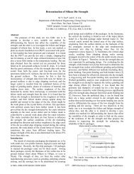
5.10E-015.05E-01Amplitude (V)5.00E-014.95E-014.90E-014.85E-010.00E+00 5.00E+07 1.00E+08 1.50E+08 2.00E+08 2.50E+08 3.00E+08Frequency (Hz)mag(Vin)Vcomm+VdiffFigure 3: Representation of common mode signals intwisted pair cablesFor pure common mode signals, the magnitudes are equal and phasedifference is 0 degrees. It is the “unwanted” signal that does notcarry any information. This is a signal that is common to all thewires in a cable. It can be represented as the algebraic averagebetween the voltages in a pair:V average = ( V 1 + V 2 )/2 (2)Since common mode currents require a return path, the grounddiffers upon its location of installation. The resulting balance of thecable is hence dependent on the effective ground. In the presentsimulation the local average of the voltages is taken as the referenceand the common mode voltage is defined as the difference betweenthe average voltage shown in (2) and the reference voltage and isgiven by (3).Figure 4: Comparison between applied differential signaland the combined differential and common modecomponents measured at the same end.3. Evaluation of differential and commonmode signal components3.1 Terminated caseIt is evident that, for a given UTP cable, there are four differentialmode components and four common mode components. Thetransmitted differential and common mode voltages evaluated in a10m cable is displayed in figures 5(a) to 5(f). The multiple curvesrepresent the amplitudes of these signals as they propagate along thecable. The far end of this cable is terminated in its characteristicimpedance.V reference = (V 1 + V 2 + V 3 + V 4 + V 5 + V 6 + V 7 + V 8 )/8 (3)V common = V average - V reference (4)Apart from these two modes, there also exists a pair to pairdifferential mode which is the signal from one pair to the other.Since the common mode current is the major cause of radiation intwisted pairs predictions[4] of radiated emissions based on onlydifferential mode currents is not correct. Also, the voltages at theinput end of the cable are not equal to each other but the sum of thedifferential and common mode component of the applied signal[5].In the current simulation the far end of the pair in which the signal isapplied was terminated in its characteristic impedance and thevoltages at the input end and the sum of the common-mode anddifferential mode measured for comparison.V input = V diff + V common (5)The maxima and minima in the above graph are not due to animpedance mismatch but because we are trying to match a pureresistor with the impedance of the cable [6] which is a complexquantity with both resistive and reactive parts. This is bound to failbut the fact that the input voltage can be defined as the sum of thesetwo modes is demonstrated here using the above model.Figure 5 (a): Diff signal on Tx pairInternational Wire & Cable Symposium 513 Proceedings of the 56th IWCS

Figure 5 (b): Diff signal on neighboring pair 1Figure 5 (e): Common mode signal on Tx pairFigure 5 (c): Diff signal on neighboring pair 2Figure 5 (f): Common mode on neighboring pair 1Figure 5 (d): Diff signal on neighboring pair 3Figure 5 (g): Common mode on neighboring pair 2International Wire & Cable Symposium 514 Proceedings of the 56th IWCS

Figure 5 (h): Common mode on neighboring pair 3Figure 6(b): Diff signal on neighboring pair13.2 Unterminated caseThe termination was changed to a value which is much larger thanthe characteristic impedance for the same length of the cable inorder to evaluate the relative differential and common modesignal strengths. As expected, the differential signal travelingthrough the transmitting pair encounters the impedance mismatchat the end of the cable and the reflected signals (Gaussian likewaves with smaller amplitudes than that of the transmitted signalsshown by dotted line in figures 6 (a-h)) reaches the input end ofthe cable. The far end voltage is equal to the sum of thetransmitted and reflected signals. As seen, from the otherpropagation modes in figures (b) to (h), the major differences inamplitudes between the terminated case and the open circuit existonly in strength of the reflected signals as opposed to thetransmitted signals.Figure 6(c): Diff signal on neighboring pair2Figure 6(a): Diff signal on Tx pairFigure 6(d): Diff signal on neighboring pair3International Wire & Cable Symposium 515 Proceedings of the 56th IWCS

Figure 6(e): Common mode on Tx pairFigure 6(f): Common mode on neighboring pair1Figure 6(h): Common mode on neighboring pair34. Balance – Unbalance conversion factorfor UTP cablesAnother method of determining the cable balance-unbalanceconversion is by the use of factors such as transverse conversionloss (TCL) and transverse conversion transfer loss (TCTL). Thefirst parameter, TCL measures the amount of differential(transverse) signal converting to longitudinal (common mode)signal in the cabling. The inverse of these two parameters arecalled LCL and LCTL respectively. The only difference betweenthese two sets of measurements is the type of applied andmeasured signal. In TCL and TCTL, a differential signal isapplied and the resulting common-mode signals measured at thenear (Vicomm) and far end (Vocomm) of the cable. Whereas, inLCL and LCTL measurements, the applied signal is commonmodeand the resulting differential signal measured at the nearand far ends. These parameters are represented in their equationform as follows:TCL = -20 * Log (Vicomm/Vinput) (6)TCTL = - 20*Log (Vocomm/Vinput) (7)Figure 7 and 8 show the frequency characteristics of TCL andTCTL for cable lengths of 10, 20, 30 and 80m. Since the inputvoltages are close to the balanced condition, they are above thestandard limit for allowable TCL (Brown curve in figure 7) forfrequencies between (1 and 200 MHz).TCL [dB]100908070605040302010Figure 6(g): Common mode on neighboring pair200 50 100 150 200 250Frequency (MHz)TCL_10m TCL_20m TCL_30m TCL_80m Mimimum TCL from standardsFigure 7: Frequency characteristics of TCL for 10, 20, 30and 80m cableInternational Wire & Cable Symposium 516 Proceedings of the 56th IWCS

807060dB TCTL504030200 50 100 150 200 250 300Frequency (MHz)TCTL_10 TCTL_20 TCTL_30 TCTL_80Figure 8: Frequency characteristics of TCTL for 10, 20, 30and 80m cableIn order to simulate unbalance in the cable, a 50pF lumped elementand 1pF was inserted at the far end of a 10m cable. As seen in figure16, there is deterioration in TCTL characteristics for the 50pF asexpected due to higher unbalance with respect to ground whencompared to the balanced case and when 1pF element has beeninserted.TCTL [dB]7060504030201000 50 100 150 200 250 300Frequency (MHz)TCTL with 50pF capacitance insertedTCTL with 1pF insertedFigure 9: TCTL with 50pF capacitance element inserted5. Numerical modeling of horizontal cable,connector and patch cableThe purpose of this section is to evaluate the RLC parameters forhorizontal cable – connector – patch cable assembly. This wouldfurther enhance the factors taken into consideration in themodeling technique described above and also study the effects ofthese connectors for its contribution towards conversion losses forthe entire system. As shown in figure 10, the model includes (1)structured cable untwisted at the end to fit into the 8 pins of theconnector, (2) the plug-connector mated assembly and (3) thepatch cable folding back from untwisted to twisted section.We are currently working on simulating the effects of thisassembly to evaluate the overall performance of the cablingsystem.Figure 10: Horizontal cable – mated connector – patchcable assembly modeled in Ansoft Maxwell©6. ConclusionsWe have presented in this paper, the use of combined finite elementand circuit extraction technique for the evaluation of differential andcommon mode signals in each of the four pairs with respect to timeand distance. The importance of introducing common mode signalsin measurements for evaluating the balance of the system isillustrated. Next, the balance-unbalance conversion factors like TCLand TCTL for various cable lengths and terminations wereevaluated. Also, unbalance elements were introduced to see theireffects on these characteristics in the frequency domain.Finally, a 3D model of the SCS-plug connector assembly- patchcable assembly has been produced and work is underway toevaluate the contribution of these components in evaluating theoverall system balance using the described technique.7. AcknowledgmentsThe authors would like to thank the Department of Trade andIndustry, U.K for the financial assistance offered towards theproject.8. References[1] S. Dorai and A.J. Peyton, “Mixed 3D finite element andcircuit based modeling of unshielded twisted pairs,” Appliedcomputational electromagnetic society, Verona, Italy (2007).[2] M. Josefsson, M.Lindstrom, J.Poltz, J. Beckett, “Statisticalanalysis of unbalance and crosstalk in TP cables”,Proceedings of the 53 rd International Wire and Cablesymposium, 2004.[3] J. Poltz, D. Gleich, M. Josefsson, M. Lindstrom,“Electromagnetic modeling of twisted pair cables”,Proceedings of the 49 th International Wire and Cablesymposium, 2000.[4] C.R. Paul, “ A Comparison of the contributions of commonmoderadiations in radiated emissions” IEEE Trans. EMC,vol.EMC-31 , no.2, pp 189-193,1989.[5] S.Hamada, T.K., J. Ochura, M. Maki, Y. Shimoshio and M.Tokuda, “Influence on Balance-Unbalance conversion factoron radiated emission characteristics of balanced cables”,IEEE, 2001.[6] R.Lao, “The twisted pair telephone transmission line”, Highfrequency electronics, 2002.International Wire & Cable Symposium 517 Proceedings of the 56th IWCS