Digital Signal Processing Chapter 7: Parametric Spectrum Estimation
Digital Signal Processing Chapter 7: Parametric Spectrum Estimation Digital Signal Processing Chapter 7: Parametric Spectrum Estimation
The power of the remaining prediction-error isMin{E{|E(k)| 2 }} = σ 2 X − rH XXR −1XXr XX .Rewriting the equation using the coefficient-vector p results inMin{E{|E(k)| 2 }} = σ 2 X − rH XXp.Linear Prediction Page 8
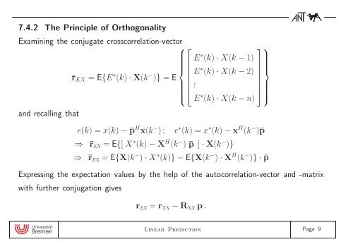
7.4.2 The Principle of OrthogonalityExamining the conjugate crosscorrelation-vector⎧⎡⎪⎨¯r EX = E{E ∗ (k) · X(k − )} = E⎢⎣⎪⎩and recalling thatE ∗ (k) · X(k − 1)E ∗ (k) · X(k − 2).E ∗ (k) · X(k − n)⎤⎫⎪⎬⎥⎦⎪⎭e(k) = x(k) − ¯p H x(k − ) ; e ∗ (k) = x ∗ (k) − x H (k − )¯p⇒ ¯r EX = E{[ X ∗ (k) − X H (k − ) ¯p ] · X(k − )}⇒ ¯r EX = E{X(k − ) · X ∗ (k)} − E{X(k − ) · X H (k − )} · ¯pExpressing the expectation values by the help of the autocorrelation-vector and -matrixwith further conjugation givesr EX = r XX − R XX p .Linear Prediction Page 9
- Page 1 and 2: transparencies - lecture: Digital S
- Page 3 and 4: 7.2 Markov Process as an Example fo
- Page 5 and 6: Past values x(k − 1), · · · ,x
- Page 7: Conjugating all elements yields inI
- Page 11 and 12: 7.4 Linear Prediction (Overview)app
- Page 13 and 14: 7.5 Levinson-Durbin Recursion∑A r
- Page 15 and 16: ecursion for the predictive coeffic
- Page 17 and 18: Levinson-Durbin Recursion• initia
- Page 19 and 20: 7.6 The Lattice-Structure7.6.1 Anal
- Page 21 and 22: Lattice Structure:• (r + 1)th sta
- Page 23 and 24: 7.6.3 Minimal Phase - Stability•
- Page 25 and 26: Br B q (0) = σ2 ∑q+1rγ rν=1a q
- Page 30 and 31: 2. Covariance Method• disadvantag
- Page 32 and 33: N−1∑k=rN−1∂ ∑N−1∑[e r
- Page 34 and 35: • rth iteration:⎡⎢⎣1â r,1
- Page 36 and 37: 7.8 Examples for Parametric Spectru
- Page 38 and 39: • application for speech codingso
- Page 40 and 41: example 3:vowel ”a”, german mal
- Page 42: example 5:comparison parametric ←
7.4.2 The Principle of OrthogonalityExamining the conjugate crosscorrelation-vector⎧⎡⎪⎨¯r EX = E{E ∗ (k) · X(k − )} = E⎢⎣⎪⎩and recalling thatE ∗ (k) · X(k − 1)E ∗ (k) · X(k − 2).E ∗ (k) · X(k − n)⎤⎫⎪⎬⎥⎦⎪⎭e(k) = x(k) − ¯p H x(k − ) ; e ∗ (k) = x ∗ (k) − x H (k − )¯p⇒ ¯r EX = E{[ X ∗ (k) − X H (k − ) ¯p ] · X(k − )}⇒ ¯r EX = E{X(k − ) · X ∗ (k)} − E{X(k − ) · X H (k − )} · ¯pExpressing the expectation values by the help of the autocorrelation-vector and -matrixwith further conjugation givesr EX = r XX − R XX p .Linear Prediction Page 9


