Digital Signal Processing Chapter 7: Parametric Spectrum Estimation

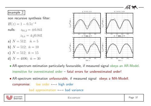
example 2:non recursive synthesis filter:H(z) = 1 − 0.5z −4nulls: z 01,2 = ±0.841z 3,4 = ±j0.841a) N = 512; ˆn = 5b) N = 512; ˆn = 10c) N = 512; ˆn = 15d) N = 4096; ˆn = 30Ŝ xx (e jΩ )/dB →Ŝ xx (e jΩ )/dB →a) N=512, ˆn=51086420-2-4-6-8-100 0.2 0.4 0.6 0.8 1c) N=512, Ω/π →ˆn=151086420-2-4-6-8-100 0.2 0.4 0.6 0.8 1Ω/π →Ŝ xx (e jΩ )/dB →Ŝ xx (e jΩ )/dB →b) N=512, ˆn=101086420-2-4-6-8-100 0.2 0.4 0.6 0.8 1d) N=4096, Ω/π →ˆn=301086420-2-4-6-8-100 0.2 0.4 0.6 0.8 1Ω/π →• AR-spectrum estimation particularly favourable, if measured signal obeys an AR-Model.insensitive for overestimated order – fatal errors for underestimated order!• AR-spectrum estimation unfavourable, if measured signal obeys a MA-Modell.compromise: low order ←→ high orderbad approximation ←→ bad varianceExamples Page 37