Digital Signal Processing Chapter 7: Parametric Spectrum Estimation
Digital Signal Processing Chapter 7: Parametric Spectrum Estimation Digital Signal Processing Chapter 7: Parametric Spectrum Estimation
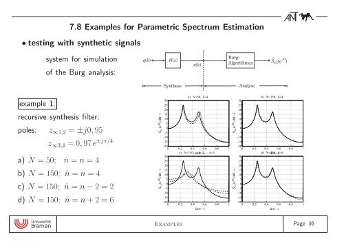
7.8 Examples for Parametric Spectrum Estimation• testing with synthetic signalssystem for simulationof the Burg analysis:example 1:recursive synthesis filter:poles: z ∞1,2 = ±j0, 95z ∞3,4 = 0, 97 e ±jπ/4a) N = 50; ˆn = n = 4b) N = 150; ˆn = n = 4c) N = 150; ˆn = n − 2 = 2d) N = 150; ˆn = n + 2 = 6Ŝ xx (e jΩ )/dB →Ŝ xx (e jΩ )/dB →a) N=50, ˆn=4302520151050-5-10-15-200 0.2 0.4 0.6 0.8 1c) N=150, --- Ω/π ˆn=2, → -⋅- ˆn=3302520151050-5-10-15-200 0.2 0.4 0.6 0.8 1Ω/π →Ŝ xx (e jΩ )/dB →Ŝ xx (e jΩ )/dB →b) N=150, ˆn=4302520151050-5-10-15-200 0.2 0.4 0.6 0.8 1d) N=150, Ω/π →ˆn=6302520151050-5-10-15-200 0.2 0.4 0.6 0.8 1Ω/π →Examples Page 36
example 2:non recursive synthesis filter:H(z) = 1 − 0.5z −4nulls: z 01,2 = ±0.841z 3,4 = ±j0.841a) N = 512; ˆn = 5b) N = 512; ˆn = 10c) N = 512; ˆn = 15d) N = 4096; ˆn = 30Ŝ xx (e jΩ )/dB →Ŝ xx (e jΩ )/dB →a) N=512, ˆn=51086420-2-4-6-8-100 0.2 0.4 0.6 0.8 1c) N=512, Ω/π →ˆn=151086420-2-4-6-8-100 0.2 0.4 0.6 0.8 1Ω/π →Ŝ xx (e jΩ )/dB →Ŝ xx (e jΩ )/dB →b) N=512, ˆn=101086420-2-4-6-8-100 0.2 0.4 0.6 0.8 1d) N=4096, Ω/π →ˆn=301086420-2-4-6-8-100 0.2 0.4 0.6 0.8 1Ω/π →• AR-spectrum estimation particularly favourable, if measured signal obeys an AR-Model.insensitive for overestimated order – fatal errors for underestimated order!• AR-spectrum estimation unfavourable, if measured signal obeys a MA-Modell.compromise: low order ←→ high orderbad approximation ←→ bad varianceExamples Page 37
- Page 1 and 2: transparencies - lecture: Digital S
- Page 3 and 4: 7.2 Markov Process as an Example fo
- Page 5 and 6: Past values x(k − 1), · · · ,x
- Page 7 and 8: Conjugating all elements yields inI
- Page 9 and 10: 7.4.2 The Principle of Orthogonalit
- Page 11 and 12: 7.4 Linear Prediction (Overview)app
- Page 13 and 14: 7.5 Levinson-Durbin Recursion∑A r
- Page 15 and 16: ecursion for the predictive coeffic
- Page 17 and 18: Levinson-Durbin Recursion• initia
- Page 19 and 20: 7.6 The Lattice-Structure7.6.1 Anal
- Page 21 and 22: Lattice Structure:• (r + 1)th sta
- Page 23 and 24: 7.6.3 Minimal Phase - Stability•
- Page 25 and 26: Br B q (0) = σ2 ∑q+1rγ rν=1a q
- Page 30 and 31: 2. Covariance Method• disadvantag
- Page 32 and 33: N−1∑k=rN−1∂ ∑N−1∑[e r
- Page 34 and 35: • rth iteration:⎡⎢⎣1â r,1
- Page 38 and 39: • application for speech codingso
- Page 40 and 41: example 3:vowel ”a”, german mal
- Page 42: example 5:comparison parametric ←
7.8 Examples for <strong>Parametric</strong> <strong>Spectrum</strong> <strong>Estimation</strong>• testing with synthetic signalssystem for simulationof the Burg analysis:example 1:recursive synthesis filter:poles: z ∞1,2 = ±j0, 95z ∞3,4 = 0, 97 e ±jπ/4a) N = 50; ˆn = n = 4b) N = 150; ˆn = n = 4c) N = 150; ˆn = n − 2 = 2d) N = 150; ˆn = n + 2 = 6Ŝ xx (e jΩ )/dB →Ŝ xx (e jΩ )/dB →a) N=50, ˆn=4302520151050-5-10-15-200 0.2 0.4 0.6 0.8 1c) N=150, --- Ω/π ˆn=2, → -⋅- ˆn=3302520151050-5-10-15-200 0.2 0.4 0.6 0.8 1Ω/π →Ŝ xx (e jΩ )/dB →Ŝ xx (e jΩ )/dB →b) N=150, ˆn=4302520151050-5-10-15-200 0.2 0.4 0.6 0.8 1d) N=150, Ω/π →ˆn=6302520151050-5-10-15-200 0.2 0.4 0.6 0.8 1Ω/π →Examples Page 36


