Finding Knees in Multi-objective Optimization

Finding Knees in Multi-objective Optimization
Jürgen Branke 1 , Kalyanmoy Deb 2 , Henning Dierolf 1 , and Matthias Osswald 1
1 Institute AIFB, University of Karlsruhe, Germany
branke@aifb.uni-karlsruhe.de
2 Department of Mechanical Engineering, IIT Kanpur, India
deb@iitk.ac.in
KanGAL Report Number 2004010
Abstract. Many real-world optimization problems have several, usually conflicting
objectives. Evolutionary multi-objective optimization usually solves this
predicament by searching for the whole Pareto-optimal front of solutions, and
relies on a decision maker to finally select a single solution. However, in particular
if the number of objectives is large, the number of Pareto-optimal solutions
may be huge, and it may be very difficult to pick one “best” solution out of this
large set of alternatives. As we argue in this paper, the most interesting solutions
of the Pareto-optimal front are solutions where a small improvement in one objective
would lead to a large deterioration in at least one other objective. These
solutions are sometimes also called “knees”. We then introduce a new modified
multi-objective evolutionary algorithm which is able to focus search on these
knee regions, resulting in a smaller set of solutions which are likely to be more
relevant to the decision maker.
1 Introduction
Many real-world optimization problems involve multiple objectives which need to be
considered simultaneously. As these objectives are usually conflicting, it is not possible
to find a single solution which is optimal with respect to all objectives. Instead, there
exist a number of so called “Pareto-optimal” solutions which are characterized by the
fact that an improvement in any one objective can only be obtained at the expense of
degradation in at least one other objective. Therefore, in the absence of any additional
preference information, none of the Pareto-optimal solutions can be said to be inferior
when compared to any other solution, as it is superior in at least one criterion.
In order to come up with a single solution, at some point during the optimization
process, a decision maker (DM) has to make a choice regarding the importance of different
objectives. Following a classification by Veldhuizen [16], the articulation of preferences
may be done either before (a priori), during (progressive), or after (a posteriori)
the optimization process.
A priori approaches basically transform the multi-objective optimization problem
into a single objective problem by specifying a utility function over all different criteria.
However, they are usually not practicable, since they require the user to explicitly and
exactly weigh the different objectives before any alternatives are known.

Most Evolutionary Multi-Objective Optimization (EMO) approaches can be classified
as a posteriori. They attempt to discover the whole set of Pareto-optimal solutions
or, if there are too many, at least a well distributed set of representatives. Then, the
decision maker has to look at this potentially huge set of Pareto-optimal alternative solutions
and make a choice. Naturally, in particular if the number of objectives is high,
this is a difficult task, and a lot of research has been done to support the decision maker
during this selection step, see e.g. [14].
Hybrids between a priori and a posteriori approaches are also possible. In this case,
the DM specifies his/her preferences as good as possible and provides imprecise goals.
These can then be used by the EMO algorithm to bias or guide the search towards the
solutions which have been classified as “interesting” by the DM (see e.g. [2, 9, 1]). This
results in a smaller set of more (to the DM) interesting solutions, but it requires the DM
to provide a priori knowledge.
The idea of this paper to do without a priori knowledge and instead to “guess” what
solutions might be most interesting for a decision maker. Let us consider the simple
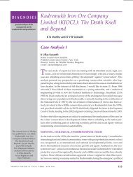
Pareto-optimal front depicted in Figure 1, with two objectives to be minimized. This
front has a clearly visible bump in the middle, which is called a “knee”. Without any
knowledge about the user’s preferences, it may be argued that the region around that
knee is most likely to be interesting for the DM. First of all, these solutions are characterized
by the fact that a small improvement in either objective will cause a large
deterioration in the other objective, which makes moving in either direction not very
attractive. Also, if we assume linear preference functions, and (due to the lack of any
other information) furthermore assume that each preference function is equally likely,
the solutions at the knee are most likely to be the optimal choice of the DM. Note that
in Figure 1, due to the concavity at the edges, similar reasoning holds for the extreme
solutions (edges), which is why these should be considered knees as well.
Fig. 1. A simple Pareto-optimal front with a knee.

In this paper, we present two modifications to EMO which allow to focus search
on the aforementioned knees, resulting in a potentially smaller set of solutions which,
however, are likely to be more relevant to the DM.
The paper is structured as follows: In the following section, we briefly review
some related work. Then, Section 3 describes our proposed modifications. The new approaches
are evaluated empirically in Section 4. The paper concludes with a summary
and some ideas for future work.
2 Related Work
Evolutionary multi-objective optimization is a very active research area. For comprehensive
books on the topic, the reader is referred to [8, 4].
The problem of selecting a solution from the set of Pareto-optimal solutions has
been discussed before. Typical methods for selection are the compromise programming
approach [17], the marginal rate of substitution approach [15], or the pseudo-weight
vector approach [8].
The importance of knees has been stressed before by different authors, see e.g. [15,
9, 6]. In [14], an algorithm is proposed which determines the relevant knee points based
on a given set of non-dominated solutions.
The idea to focus on knees and thereby to better reflect user preferences is also
somewhat related to the idea of explicitly integrating user preferences into EMO approaches,
see e.g. [3, 1, 5, 12].
3 Focusing on Knees
In this section, we will describe two modifications which allow the EMO-approach to
focus on the knee regions, which we have argued are, given no additional knowledge,
the most likely to be relevant to the DM.
We base our modifications on NSGA-II [10], one of today’s standard EMO approaches.
EMO approaches have to achieve two things: they have to quickly converge
towards the Pareto-optimal front, and they have to maintain a good spread of solutions
on that front. NSGA-II achieves that by relying on two measures when comparing individuals
(e.g. for selection and deletion): The first is the non-domination rank, which
measures how close an individual is to the non-dominated front. An individual with a
lower rank (closer to the front) is always preferred to an individual with a higher rank. If
two individuals have the same non-domination rank, as a secondary criterion, a crowding
measure is used, which prefers individuals which are in rather deserted areas of the
front. More precisely, for each individual the cuboid length is calculated, which is the
sum of distances between an individual’s two closest neighbors in each dimension. The
individuals with greater cuboid length are then preferred.
Our approach modifies the secondary criterion, and replaces the cuboid length by
either an angle-based measure or a utility-based measure. These will be described in the
following subsections.

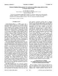
Fig. 2. Calculation of the angle measure. The standard version just calculates α, the intensified
version takes 4 neighbors into account and calculates the maximum of α β γ, and δ.
3.1 Angle-based Focus
In the case of only two objectives, the trade-offs in either direction can be estimated
by the slopes of the two lines through an individual and its two neighbors. The angle
between these slopes can be regarded as an indication of whether the individual is at
a knee or not. For an illustration, consider Figure 2 (a). Clearly, the larger the angle α
between the lines, the worse the trade-offs in either direction, and the more clearly the
solution can be classified as a knee.
More formally, to calculate the angle measure for a particular individual xi, we
calculate the angle between the individual and its two neighbors, i.e. between ¡ xi¢ 1£ xi¤
and ¡ xi £ xi¥ 1¤ . These three individuals have to be pairwise linearly independent, thus
duplicate individuals (individuals with the same objective function values, which are
not prevented in NSGA-II per se) are treated as one and are assigned the same anglemeasure.
If no neighbor to the left (right) is found, a vertical (horizontal) line is used to
calculate the angle. Similar to the standard cuboid-length measure, individuals with a
larger angle-measure are preferred.
To intensify the focus on the knee area, we also suggest a variant which uses four
neighbors (two in either direction) instead of two. In that case, four angles are computed,
using on either side either the closest or the second closest neighbor (cf. angles.
α£ β£ γ£ δ in Figure 2). The largest of these four angles is then assigned to the individual.
Calculating the angle measure in 2D is efficient. For more than two objectives, however,
it becomes impractical even to just find the neighbors. Thus, we restrict our examination
of the angle-based focus to problems with two objectives only. The utility-based
focus presented in this section, however, can be extended to any number of objectives.
3.2 Utility-based Focus
An alternative measure for a solution’s relevance could be the expected marginal utility
that solution provides to a decision maker, assuming linear utility functions of the form
U ¡ ¡ ¡ ¡
x¤©¨ λ � λ¤ f1
x¤ 1 f2 , with ��� 0£ 1� all λ being equally likely. x£ 뤧¦ For illustration,
let us first assume we would know that the DM has a particular preference function
U ¡ , with some λ� known . Then, we could calculate, for each individual xi in x£ λ� ¤ the
population, the DM’s utility U ¡ xi of that individual. Clearly, given the choice among
£ λ� ¤
all individuals in the population, the DM would select the one with the highest utility.

Now let us define an individual’s marginal utility U�
¡ x£ λ� ¤ as the additional cost the
DM would have to accept if that particular individual would not be available and he/she
would have to settle for the second best, i.e.
¡
xi£ λ� ¤�¦ U�
�
� j� min iU ¡ £ λ� ¤ � x j U ¡ ¤ xi£ ¦ λ� : i argminU ¡ £ λ� ¤ x j
0 : otherwise
The utility measure we propose here assumes a distribution of utility functions uniform
in the parameter λ in order to calculate the expected marginal utility. For the case
of only two objectives, the expected marginal utility can be calculated exactly by integrating
over all possible linear utility functions as follows: Let us denote with xi the
solution on position i if all solutions are sorted according to criterion f1. Furthermore,
let λi� j be the weighting of objectives such that solutions xi and x j have the same utility,
i.e.
¡ ¡
j¤ � f2 xi¤ x f2
¡ ¡ ¡
f1 f1 j¤�¨ x f2 j¤ � x � xi¤ f2
j ¦
¡ λi�
xi¤
Then, the expected marginal utility of solution xi can be calculated as
E ¡ ¡
xi£ λ¤�¤�¦��
U�
1� 1 λi� i�
α� α
i λi� 1� ¡ ¡ ¡
� f1 xi¢ 1¤�¤�¨
xi¤ f1
¨ �
i� λi� 1
α� α
i� 1 λi� 1� ¡ ¡ ¡
� f1 xi¢ 1¤�¤�¨
xi¤ f1
¡ 1 � α¤
¡ 1 � α¤
¡ ¡ ¡
� f2 xi¢ 1¤�¤ f2 xi¤ dα
¡ ¡ ¡
� f2 xi¢ 1¤�¤ f2 xi¤ dα
Unlike the angle measure, the utility measure extends easily to more than two objectives,
by defining U ¡ ¡
∑λi fi x¤ with ∑λi ¦ 1. The expected marginal utilities
x£ λ¤�¦
can be approximated simply by sampling, i.e. by calculating the marginal utility for all
individuals for a number of randomly chosen utility functions, and taking the average
as expected marginal utility. Sampling can be done either randomly or, as we have done
in order to reduce variance, in a systematic manner (equi-distant values for λ). We call
the number of utility functions used for approximation precision of the measure. From
our experience, we would recommend a precision of at least the number of individuals
in the population.
Naturally, individuals with the largest overall marginal utility are preferred. Note,
however, that the assumption of linear utility functions makes it impossible to find knees
in concave regions of the non-dominated front.
4 Empirical evaluation
Let us now demonstrate the effectiveness of our approach on some test problems. The
test problems are based on the DTLZ ones [11, 7]. Let n denote the number of decision
variables (we use n ¦ 30 below), and K be a parameter which allows to control the
number of knees in the problem, generating K knees in a problem with two objectives.

Fig. 3. Comparison of NSGA-II with (a) angle-measure, (b) 4-angle-measure and (c) utilitymeasure
on a simple test problem.
Then, the DO2DK test problem is defined as follows:
¡
x¤�¦ min f1 g ¡ x¤ r ¡ � πx1� x1¤�� sin 2 s¥ 1 ¨ ¨�� 1 2s �
2
1
s¥ 2 � π 1� � ¨
¡
x¤�¦ min f2 g ¡ x¤ r ¡ ¡ ¡
πx1� ¨ x1¤
π¤�¨ 1¤
cos 2
g ¡ ¨ x¤�¦
�
1
n 9
n 1 ∑ xi
i � 2
1
K cos¡ 2Kπx1¤�� 2 s 2
0 � xi � 1 i ¦ 1£ 2£ ����� £ n
r ¡ x1¤�¦ 5 ¨ 10 ¡ x1 � 0� 5¤ 2 ¨
The parameter s in that function skews the front.
Let us first look at an instance with a very simple front which is convex and has a
single knee, using the parameters K ¦ 1£ n ¦ 30, and s ¦ 0. Figure 3 compares the nondominated
front obtained after running NSGA-II with the three proposed methods, the
angle-measure, the 4-angle-measure, and the utility-measure for 10 generations with a
population size of 200. As can be seen, all three methods clearly focus on the knee. The
run based on the utility-measure has the best (most regular) distribution of individuals
on the front. As expected, the 4-angle-measure puts a stronger focus on the knee than
the standard angle-measure.
Now let us increase the number of knees ¡ K ¦ 4¤ and skew the front ¡ s ¦ 1� 0¤ .
The non-dominated front obtained after 10 generations with a population size of 100 is
depicted in Figure 4. As can be seen, both measures allow to discover all knees. The
utility-measure shows a wider distribution at the shallow knees, while the angle-based
measure emphasizes the stronger knees, and also has a few solutions reaching into the
concave regions.

Fig. 4. Comparison of NSGA-II with (a) utility-measure and (b) angle-based measure on a test
problem with several knees. Populations size is 100, result after 10 generations, for utilitymeasure
a precision of 100 was used.
The DEB2DK problem is similar, but concave at the edges of the Pareto front. It is
defined as follows:
¡
x¤�¦ min f1 g ¡ x¤ r ¡ x1¤ sin ¡ 2¤ πx1�
¡
x¤�¦ min f2 g ¡ x¤ r ¡ x1¤ cos ¡ 2¤ πx1�
g ¡ x¤�¦ 1 ¨
9
� n 1
n
∑
1� xi
2
r ¡ x1¤�¦ ¨ 5 10 ¡ � 0� 5¤ x1 2 ¨
K cos¡ 2Kπx1¤
¦ 1£ � 2£ � ����� £ 0 xi 1 i n
Figure 5 again compares the resulting non-dominated front for NSGA-II with anglemeasure
and utility-measure. As with the previous function, it can be seen that the
utility-based measure has a stronger focus on the tip of the knees, while with the anglebased
measure, again there are some solutions reaching into the concave regions.
1

Fig. 5. Comparison of NSGA-II with (a) angle-measure and (b) utility-measure on a test problem
with several knees. Populations size is 200, result after 15 generations, for utility-measure a
precision of 100 was used.
Finally, let us consider a problem with 3 objectives. DEB3DK is defined as follows:
¡
x¤�¦ min f1 g ¡ x¤ r ¡ sin x1£ x2¤ ¡ sin πx1� 2¤ ¡ 2¤ πx2�
¡
x¤�¦ min f2 g ¡ x¤ r ¡ sin x1£ x2¤ ¡ cos πx1� 2¤ ¡ 2¤ πx2�
¡
x¤�¦ min f3 g ¡ x¤ r ¡ x1£ x2¤ cos ¡ πx1� 2¤
g ¡ ¨ x¤�¦
�
1
n 9
n 1 ∑ xi
i � 2
r ¡ ¡ ¡ ¡
x2¤�¦
x2¤�¤�� x1£ x1¤�¨
¡
¨ xi¤�¦
r1 r2 2
ri 5 10 ¡ � 0� 5¤ xi 2 ¨
2
K cos¡ 2Kπxi¤
¦ 1£ � 2£ � ����� £ 0 xi 1 i n
Note that this test problem can also be extended to more than three objectives as it is
based on the DTLZ functions. The number of knees then increases as K M¢ 1 , where M
is the number of objectives.
Since with three objectives, only the utility-based measure can be used, Figure 6
only shows the resulting non-dominated front for that approach. Again, NSGA-II with
utility-measure is able to find all the knee points.
5 Conclusions
Most EMO approaches attempt at finding all Pareto-optimal solutions. But that leaves
the decision maker (DM) with the challenge to select the best solution out of the potentially
huge set of Pareto-optimal alternatives. In this paper, we have argued that, without

Fig. 6. NSGA-II with utility-measure on a 3-objective problem with knees. Populations size is
150, result after 20 generations, precision is 100.
further knowledge, the knee points of the Pareto-optimal front are likely to be the most
relevant to the DM. Consequently, we have then presented and compared two different
ways to focus the search of the EA to these knee regions.
The basic idea was to replace NSGA-II’s cuboid length measure, which is used to
favor individuals in sparse regions, by an alternative measure, which favors individuals
in knee regions. Two such measures have been proposed, one based on the angle to
neighboring individuals, another one based on marginal utility.
As has been shown empirically, either method was able to focus search on the knee
regions of the Pareto-optimal front, resulting in a smaller number of potentially more
interesting solutions. The utility-measure seemed to yield slightly better results and is
easily extendable to any number of objectives.
We are currently working on a refined version of the proposed approach, which
allows to control the strength of the focus on the knee regions, and to calculate the
marginal utility exactly, rather than estimating it by means of sampling. Furthermore,
it would be interesting to integrate the proposed ideas also into EMO approaches other
than NSGA-II, and to test the presented ideas on some real-world problems.
Acknowledgments:
K. Deb acknowledges the support through Bessel Research Award from Alexander von
Humboldt Foundation, Germany during the course of this study.
The empirical results have been generated using the KEA library from the University
of Dortmund [13].

References
1. J. Branke and K. Deb. Integrating user preferences into evolutionary multi-objective optimization.
In Y. Jin, editor, Knowledge Incorporation in Evolutionary Computation. Springer,
to appear.
2. J. Branke, T. Kaußler, and H. Schmeck. Guidance in evolutionary multi-objective optimization.
Advances in Engineering Software, 32:499–507, 2001.
3. J. Branke, T. Kaußler, and H. Schmeck. Guidance in evolutionary multi-objective optimization.
Advances in Engineering Software, 32(6):499–508, 2001.
4. C. A. Coello Coello, D. A. Van Veldhuizen, and G. B. Lamont. Evolutionary Algorithms for
Solving Multi-Objective Problems. Kluwer, 2002.
5. D. Cvetković and I. C. Parmee. Preferences and their Application in Evolutionary Multiobjective
Optimisation. IEEE Transactions on Evolutionary Computation, 6(1):42–57, February
2002.
6. I. Das. On characterizing the ’knee’ of the pareto curve based on normal-boundary intersection.
Structural Optimization, 18(2/3):107–115, 1999.
7. K. Deb. Multi-objective genetic algorithms: Problem difficulties and construction of test
problems. Evolutionary Computation Journal, 7(3):205–230, 1999.
8. K. Deb. Multi-objective optimization using evolutionary algorithms. Chichester, UK: Wiley,
2001.
9. K. Deb. Multi-objective evolutionary algorithms: Introducing bias among Pareto-optimal
solutions. In A. Ghosh and S. Tsutsui, editors, Advances in Evolutionary Computing: Theory
and Applications, pages 263–292. London: Springer-Verlag, 2003.
10. K. Deb, S. Agrawal, A. Pratap, and T. Meyarivan. A fast and elitist multi-objective genetic
algorithm: NSGA-II. IEEE Transactions on Evolutionary Computation, 6(2):182–197, 2002.
11. K. Deb, L. Thiele, M. Laumanns, and E. Zitzler. Scalable multi-objective optimization test
problems. In Proceedings of the Congress on Evolutionary Computation (CEC-2002), pages
825–830, 2002.
12. G. W. Greenwood, X. S. Hu, and J. G. D’Ambrosio. Fitness Functions for Multiple Objective
Optimization Problems: Combining Preferences with Pareto Rankings. In Richard K. Belew
and Michael D. Vose, editors, Foundations of Genetic Algorithms 4, pages 437–455, San
Mateo, California, 1997. Morgan Kaufmann.
13. Ls11. The Kea-Project (v. 1.0). University of Dortmund, Informatics Department, online:
http://ls11-www.cs.uni-dortmund.de, 2003.
14. C. A. Mattson, A. A. Mullur, and A. Messac. Minimal representation of multiobjective
design space using a smart pareto filter. In AIAA/ISSMO Symposium on Multidisciplinary
Analysis and Optimization, 2002.
15. K. Miettinen. Nonlinear Multiobjective Optimization. Kluwer, Boston, 1999.
16. D. Van Veldhuizen and G. B. Lamont. Multiobjective evolutionary algorithms: Analyzing
the state-of-the-art. Evolutionary Computation Journal, 8(2):125–148, 2000.
17. P. L. Yu. A class of solutions for group decision problems. Management Science, 19(8):936–
946, 1973.