An Improved VLSI Test Economics Analysis System - Laboratory for ...

An Improved VLSI Test Economics Analysis SystemAdvisor: Cheng-Wen Wu, Ph.D.Student: Jenn-Dong LinDepartment of Electrical EngineeringNational Tsing Hua UniversityHsinchu, Taiwan, 300R.O.C.June, 1998

AbstractManagers used to consider design for testability (DFT) as an overhead in development andproduction rather than an aid. We take a full consideration on the relation between DFTmethodologies and cost/revenue models, and show that DFT may actually help engineers toshorten the total time needed in product development, which leads to lower man-power costand shorter time to market, and therefore results in more revenue through out the product'slife time. Production cost may also be reduced due to lower testing cost.Base on this, economic models are developed to model the cost and revenue of a VLSIproduct. Our system consists of a set of circuit parameters, four models, and a test methodologylibrary. The circuit parameters are normally available or easy to estimate early inthe design phase. The four models are Cost Model, Market Life Model, Time Model, andQuality Model, respectively Cost Model estimates cost, and Market Life Model estimatesrevenue. The other two models estimate parameters used by the previous two. Time Modelestimates all time related parameters, and Quality Model estimates test related parameters.Moreover, the test methodology library describes the eect of DFT on all parameters.A WWW-based VLSI test strategy planning system|the Evaluation System for TEstEngineering Methodologies (ESTEEM)|has been developed. It is an improved version ofthe system that we have developed over the past two years. The system is realized by awebbase program with secure, friendly graphic user interface and exible analysis engine.Test length and test generation time of ISCAS'89 benchmark circuits and the scanmodiedcircuits were evaluated to compare the dierence between normal and scan design.Finally, an IEEE 1149.5 MTM-Bus slave module chip is analyzed by our system. The resultshows the prot will greatly increase if DFT is used, since it saves the development timeand shortens time to market. Besides, by comparing dierent volumes for the same case, wefound a threshold volume. The total cost with DFT is lower than that without DFT underthis threshold volume.

Contents1 Introduction 11.1 Economic Models . . . . . . . . . . . . . . . . . . . . . . . . . . . . . . . . . 21.2 Analysis System . . . . . . . . . . . . . . . . . . . . . . . . . . . . . . . . . . 31.3 Previous Works . . . . . . . . . . . . . . . . . . . . . . . . . . . . . . . . . . 32 Economic Models 72.1 Notation . . . . . . . . . . . . . . . . . . . . . . . . . . . . . . . . . . . . . . 82.2 Circuit Description . . . . . . . . . . . . . . . . . . . . . . . . . . . . . . . . 92.3 Introduction to Economic Model . . . . . . . . . . . . . . . . . . . . . . . . . 142.4 Cost Model . . . . . . . . . . . . . . . . . . . . . . . . . . . . . . . . . . . . 162.4.1 Impact of Time . . . . . . . . . . . . . . . . . . . . . . . . . . . . . . 172.4.2 Impact of Volume . . . . . . . . . . . . . . . . . . . . . . . . . . . . . 202.4.3 Development Cost . . . . . . . . . . . . . . . . . . . . . . . . . . . . 202.4.4 Manufacturing Cost . . . . . . . . . . . . . . . . . . . . . . . . . . . . 242.4.5 Testing Cost . . . . . . . . . . . . . . . . . . . . . . . . . . . . . . . . 242.5 Time Model . . . . . . . . . . . . . . . . . . . . . . . . . . . . . . . . . . . . 262.6 Quality Model . . . . . . . . . . . . . . . . . . . . . . . . . . . . . . . . . . . 272.6.1 Defect Level . . . . . . . . . . . . . . . . . . . . . . . . . . . . . . . . 282.6.2 Yield . . . . . . . . . . . . . . . . . . . . . . . . . . . . . . . . . . . . 282.6.3 Fault Coverage . . . . . . . . . . . . . . . . . . . . . . . . . . . . . . 292.7 Market Life Model . . . . . . . . . . . . . . . . . . . . . . . . . . . . . . . . 322.8 Impact of Design for Testability . . . . . . . . . . . . . . . . . . . . . . . . . 33i

3 System Development 353.1 System Architecture . . . . . . . . . . . . . . . . . . . . . . . . . . . . . . . 353.2 Analysis Flow . . . . . . . . . . . . . . . . . . . . . . . . . . . . . . . . . . . 373.3 User Interface . . . . . . . . . . . . . . . . . . . . . . . . . . . . . . . . . . . 383.4 Program Algorithm . . . . . . . . . . . . . . . . . . . . . . . . . . . . . . . . 404 Experimental Result 424.1 ISCAS89 Benchmark Overview . . . . . . . . . . . . . . . . . . . . . . . . . 424.2 Model Parameters Evaluation . . . . . . . . . . . . . . . . . . . . . . . . . . 424.2.1 Fault Coverage . . . . . . . . . . . . . . . . . . . . . . . . . . . . . . 444.2.2 Area . . . . . . . . . . . . . . . . . . . . . . . . . . . . . . . . . . . . 464.3 Case Study . . . . . . . . . . . . . . . . . . . . . . . . . . . . . . . . . . . . 495 Conclusions 56A Summary of All Model 58A.1 Cost Model . . . . . . . . . . . . . . . . . . . . . . . . . . . . . . . . . . . . 58A.1.1 Developmental cost . . . . . . . . . . . . . . . . . . . . . . . . . . . . 58A.1.2 Manufacturing Cost . . . . . . . . . . . . . . . . . . . . . . . . . . . . 59A.1.3 Testing Cost . . . . . . . . . . . . . . . . . . . . . . . . . . . . . . . . 59A.2 Time Model . . . . . . . . . . . . . . . . . . . . . . . . . . . . . . . . . . . . 60A.3 Quality Model . . . . . . . . . . . . . . . . . . . . . . . . . . . . . . . . . . . 60A.4 Market Life Model . . . . . . . . . . . . . . . . . . . . . . . . . . . . . . . . 60B Fault Coverage Approximation of ISCAS'89 Benchmark 62ii

List of Figures2.1 Area relation between core and pads: (a) maximal utilization, (b) core bounded,(c) pads bounded. . . . . . . . . . . . . . . . . . . . . . . . . . . . . . . . . . 132.2 Relation of models. . . . . . . . . . . . . . . . . . . . . . . . . . . . . . . . . 142.3 Hierarchical structure of Cost Model. . . . . . . . . . . . . . . . . . . . . . . 162.4 How is cost impacted by time? . . . . . . . . . . . . . . . . . . . . . . . . . . 172.5 Continuous cost. . . . . . . . . . . . . . . . . . . . . . . . . . . . . . . . . . 192.6 General develop process. . . . . . . . . . . . . . . . . . . . . . . . . . . . . . 262.7 (a) Empirical result of FC v.s V, (b) Goel's estimation. . . . . . . . . . . . . 292.8 The market life cycle model. . . . . . . . . . . . . . . . . . . . . . . . . . . . 322.9 DFT impact on parameters. . . . . . . . . . . . . . . . . . . . . . . . . . . . 333.1 Architecture of ESTEEM. . . . . . . . . . . . . . . . . . . . . . . . . . . . . 363.2 Analysis ow of ESTEEM. . . . . . . . . . . . . . . . . . . . . . . . . . . . . 373.3 File Manager. . . . . . . . . . . . . . . . . . . . . . . . . . . . . . . . . . . . 383.4 Model Editor: (a) block parameters, (b) fault coverage and test length. . . . 393.5 Result Display. . . . . . . . . . . . . . . . . . . . . . . . . . . . . . . . . . . 404.1 Experimental and approximated result of fault coverage. . . . . . . . . . . . 444.2 Architecture of IEEE 1149.5 MTM-bus slave module. . . . . . . . . . . . . . 494.3 Relation between cost and volume. . . . . . . . . . . . . . . . . . . . . . . . 534.4 Stage cost ratio of 2k volume: (a) Original, (b) DFT. . . . . . . . . . . . . . 544.5 Stage cost ratio of 320k volume: (a) Original, (b) DFT. . . . . . . . . . . . . 54iii

List of Tables2.1 Examples of notation. . . . . . . . . . . . . . . . . . . . . . . . . . . . . . . 82.2 Type and notation of parameters in models. . . . . . . . . . . . . . . . . . . 82.3 Parameters of circuit description. . . . . . . . . . . . . . . . . . . . . . . . . 92.4 Types of block. . . . . . . . . . . . . . . . . . . . . . . . . . . . . . . . . . . 102.5 Test methodologies for each type of block. . . . . . . . . . . . . . . . . . . . 102.6 N pass and N v ratio. . . . . . . . . . . . . . . . . . . . . . . . . . . . . . . . . 254.1 ISCAS'89 benchmark circuit characteristics. . . . . . . . . . . . . . . . . . . 434.2 Fault coverage parameter approximation. . . . . . . . . . . . . . . . . . . . . 454.3 Fault coverage and test length of random pattern. . . . . . . . . . . . . . . . 474.4 Circuit area of benchmarks. . . . . . . . . . . . . . . . . . . . . . . . . . . . 484.5 Parameters of chip. . . . . . . . . . . . . . . . . . . . . . . . . . . . . . . . . 494.6 Parameters of each block. . . . . . . . . . . . . . . . . . . . . . . . . . . . . 504.7 Parameters in cost model. . . . . . . . . . . . . . . . . . . . . . . . . . . . . 504.8 Parameters of time model. . . . . . . . . . . . . . . . . . . . . . . . . . . . . 514.9 Parameters of market life model. . . . . . . . . . . . . . . . . . . . . . . . . 514.10 Parameters of quality model. . . . . . . . . . . . . . . . . . . . . . . . . . . . 514.11 Result of analysis. . . . . . . . . . . . . . . . . . . . . . . . . . . . . . . . . . 524.12 Cost of dierent volume. . . . . . . . . . . . . . . . . . . . . . . . . . . . . . 534.13 Cost of dierent volume in larger area case. . . . . . . . . . . . . . . . . . . 53iv

Chapter 1IntroductionFrom business perspective, the goal for designing a chip is to gain maximal prot frommarket. There are three key factors aecting the prot: cost, time, and quality. The costincludes design cost, manufacturing cost and testing cost. The time includes design time,test generation time, test executing time, etc. Quality includes defect level, performance andreliability. Generally, these three factors are conict to each other. For example, low defectlevel chip needs long test generation time, test executing time and high test cost. TraditionalVLSI economics only need to balance the cost of those factors to gain maximal prot.However, VLSI technology has a rapid growth of integration, which results in millionsof transistors integrated in a single chip. Such a chip is almost impossible to test withoutdesign-for-testability (DFT) consideration. By including DFT methodologies to our teststrategies, we can change the conicting situation of the three prot factors. For example,scan will reduce test generation time and increase fault coverage simultaneously, but it scanincreases chip area, i.e., it increases manufacturing cost. DFT thus results in a situationwhich is more complex than before. Selecting the best test strategy for a VLSI circuit byperforming an economic analysis becomes more and more important.In our study, we propose a set of economic models to estimate prot changes resultingfrom dierent test strategies. A new version of the analysis system which we have workedon since more than two years ago is developed. This system can help the user make DFTdecision in the early stage of the design.1

1.1 Economic ModelsIn the economic models, the prot can be estimated by anumber of circuit parameters suchas the number of gates, nets, and I/Os, and the sequential depth, routing ratio, physicaldesign rule, netlist, layout, etc. However, not all of these circuit parameters are availablein early design cycle, therefore the circuit parameters of our models must be available oreasy to estimate early in the design phase. In our study, we propose a set of such circuitparameters. Besides, some models are developed to estimate the parameters if they can notbe obtained directly in the early design stage.The prot is equal to the revenue subtracted by cost. The revenue comes from market.Thus, a Market Life Model is proposed to estimate the revenue. This model use generalproduction life cycle model to gure out relation between revenue and time to market. Thetime to market will be estimated in the Time Model. Then, we can obtain the revenue ofthe project under consideration.Cost includes capital, labor and raw material. Capital is dened as long-term investmentsuch as land, buildings, machines and tools. Labor includes man-power and management.There are dierence between capital cost and the other two costs. The labor and raw materialcosts are purchased only for immediate or current use, but capital cost is generally purchasedfor use over a long period. Thus, the reasonable capital cost is the depreciation value duringthe current project. In our study, we propose three types of cost equation: one for labor andraw material cost and the other two for capital cost.Most of our cost equations are functions of the time. For example, the salary of designman-power is proportional to the design time and the cost of tester, and the cost of testeris estimated as the depreciation during the test execution time. Some of these time relatedparameters are hard to estimate directly. We propose a Time Model to estimate theseparameters.Cost Model is proposed to estimate total cost of a project. The project is divided intothree stages: design, manufacture and test. Our model estimate each stage cost hierarchically.Each stage cost continuously divided into more and more detail item cost, then theproposed three type cost equations are selected to model each item cost. Finally, all the item2

costs are summed as the total cost.Moreover, a Quality Model is proposed to estimate some test related parameters such asfault coverage, test length, yield and defect level. Those parameters is also hard to estimatedirectly. Some parameters, such as fault coverage and test length, are dependent. Our modeldescribes the dependent relation condition of these parameters, so user can decide the valueof parameters by this model. Besides, this model estimates defect level as our test quality.Although this factor also can map to the cost, the eect of this factor need to consider over along period. We suggest user to decide a threshold defect level. If the estimated defect levelhigher than the threshold, other test methodologies should be applied to lower the defectlevel.Finally, these four models can evaluate prot form those proposed parameters. If we canknow how these parameters will be aected by various test methodologies, we can comparethe prot of these test methodologies. This is one future work. For now, we only considerscan test to obtain the changes of parameters such as test generation time, test length, chiparea, etc.1.2 Analysis SystemWe develop a software system, call ESTEEM, for the following two purposes. First, thissystem is used to implement our economic models. Second, this system can help us collectdata for future works. For these purposes, our system have the following features: theweb-based program can be accessed from any place of the world via the Internet. Securityis provided to protect data of each user. A database is integrated to handle user's data.Friendly graphic user interface (GUI) and exible analysis engine makes it easy to handleproject les and modify equations in the models.1.3 Previous WorksA knowledge based system to aid in creating easily testable VLSI chips, called TDES(Testable Design Expert System), was developed at the University of Southern California [1].It was implemented in Lisp. The aim of TDES was to create a framework for methodol-3

ogy incorporating structural, behavioral, qualitative and quantitative aspects of known DFTtechniques.The successor of TDES is TIGER (Testability Insertion Guidance ExpeRt [2]), whichis now an industrial tool. It handles gate level descriptions, and uses a more sophisticatedpartitioning process than TDES. It uses a similar weighting system to evaluate embedding,mainly in terms of area overhead, estimated test pattern generation (TPG) eort, and estimatedtest time.Brendan Davis proposed EVALUATE [3] which is a decision support tool mainly forthe manufacturing test strategy part of the overall test strategy in 1994. It also includesthe design to test strategy and the eld-service strategy. Since EVALUATE produces anindication of the likely number of defects that will `escape' to the eld for each dierentstrategy analyzed, it eectively provides a measure of the eld-service workload also.1995, Dislis et al. proposed test strategy planners called ECOtest and ECOvbs [4]. TheECOvbs applied the same principles of economics to board designs as ECOtest did to ASICdesigns. It fully calculated the economic and technical eects of test method and also oerssome design optimization and a range of dierent test strategy planning algorithms.All of above papers estimate test cost of well-designed circuits. However, many DFTmethods must be applied before detailed design. Models should not use the parameterswhich is dicult to obtain or estimate in the oor-planning stage. Kim [5] proposed a testcost prediction model which estimates the cost of IC testing in a manufacturing environment.This model predicts chip testing cost and quality of test using a set of circuit manufacturingparameters. Those parameters are available at the early stage of the design cycle. But, theirmodel did not consider the condition of DFT.In [6], another cost model called CMU Test Cost model was proposed. Then, this modelwas used with a range of parameters representing typical industrial conditions to nd athreshold volume. This volume indicates if we get benet from DFT. They found thatcost and benet of DFT is strongly aected by the volume. Similar result was obtained byWei [7]. This paper just found the relation among DFT related parameters, cost and volume.However, they did not describe how DFT methodologies aects these parameters.In our research group, the "Evaluation System for TEst Engineering methodologies (ES-4

TEEM)" for VLSI test strategy planning [7,8], has been developed to accomplish the analysisprocess of test strategy planning. This system uses cost models to calculate the overall costand a test methodologies library to oer suitable test methods for various circuits. However,the original version [8] used some parameters that can only be obtained after the design wasdone.The web-based version of ESTEEM [7] used Java to provide a cross-platform standardgraphic user interface (GUI) environment, and users can perform analysis by web browservia the Internet. Besides, it integrates a Standard Query Language (SQL) database serverto handle the user's data. However, the pure Java system is not stable enough while it itaccessed on the browser. We propose a more stable system in our study.Base on the previous works, we add a quality model to calculate more precise values oftest related parameters, such as fault coverage, yield and defect level. The whole system nowincludes four models: Cost Model, Time Model, Quality Model and Market Life Model. Inthe Cost Model, we propose three basic cost types to estimate costs, and divide test cost intothree stages: wafer test, pre-burn-in test and nal test. Besides, in the circuit description,we propose many suggestion and heuristic to help the user estimate circuit parameters whichare hard to obtain. The economic models will be detailed in Chapter 2 and summarized inAppendix A.The new version of ESTEEM provides more security to user data. The system uses Perl,Java and Javascript languages and integrates web server, SQL server, and CGI programs.This system provides more friendly user interface, such as le manager, model editor, andresult display. Besides, a more powerful analysis engine is developed, so user can easily addnew equations or modify proposed models to t the condition of their companies. Moredetails will be discussed in Chapter 3.Moreover, the ISCAS'89 were applied to sequential ATPG and random pattern fault simulator.Then, ISCAS'89 SCAN were applied to combinational ATPG. Test length and testgeneration time of normal circuits and its scan-modied circuits were evaluated to comparethe dierence between them. Then, ISCAS'89 circuits were translated to verilog format tosynthesis. The synthesized area of ISCAS'89 and its scan version were compared.Finally, an IEEE 1149.5 MTM-Bus slave module chip is analyzed by our system [9].5

The result shows the DFT prot will greatly increase if DFT is used, since it saves thedevelopment time and shortens time to market. Besides, by comparing dierent volumes forthe same case, we found a threshold volume. The total cost with DFT is lower than thatwithout DFT under this threshold volume.6

Chapter 2Economic ModelsIn this chapter, we propose our economic models to estimate prot and quality of a testingstrategy during the oor-planning stage. In general, estimation is wildly used to predictresults in advance. Models of the interested system should be built up before estimationresults can be obtained. The way how models are created strongly aects the precision ofsimulation. Minor information is dropped to reduce the computing complexity in the processof modeling. In fact, there is a close correspondence between complexity on one hand andprecision on the other hand, so a variety of models are constructed for trade-os betweenthem. Moreover, the lack of detailed information in the early stage of estimation impedescreating precise models. In our economic models, there are some empirical parameters,including design complexity, reusability, and testability, etc. These parameters are vague atthe rst sight. But experienced designers, in practice, can always obtain reasonable gures.In addition, our system collects such parameters of various designs into a database to helpthe users perform estimation according to similar designs.Finally, the goal of our system is not to provide exact prediction of the prot, predictingrelative economic metric among various testing strategies. It will be a great help for makingclever decisions of testing strategies before the design process.This chapter is organized as follows. In the rst section, we briey dene the notationused in this paper. In the second section, the terminology of circuit description is introduced.In the third section, the concept of the whole economic model is described. The economicmodels are the Cost Model, the Time Model, the Market Life Model and the Quality Model.We discuss these four models in the following four sections, respectively. Finally, impact of7

DFT methodologies will be shown in the last section.2.1 NotationIn this section, we dene notation of the variables used in this paper. The variables aredesigned by the following two rules.Rule 1: A Capital letter represents a chip-level parameter and a small letter represents ablock-level one.For example: g is the gate count of a block and G is the gate count of a chip.Rule 2: Three parts compose a variable.A variable has the following basic form: Ts i , where the capital letter T , the smallletter s, and the subscript i represent the Type, the Stage, and the Item of theparameter, respectively. Examples of the notation are listed in Table 2.1. Sometimes,the stage can be implied by the item. For example, U wafer (cost per wafer) is obviouslyin manufacture stage, so we do not need to include this part in the notation. However,Cd mang(design management cost) must indicate the development stage explicitly,because management cost may occur during development and manufacturing stages.Table 2.2 lists some general types of parameters and their notation.Table 2.1: Examples of notation.Notation Type Stage Item DescriptionCd mang Cost Development Management Development management costTt f Time Test Final Final test timeU wafer Unit Cost Manufacturing Wafer Productive cost per waferTable 2.2: Type and notation of parameters in models.Notation Type ExampleC Cost Cd Development costR Ratio Rd mang Development management time ratioK User Dene Kd User dene development costT Time Td Development timeN Number Nv Volume to deliverU Unit Cost Ud eng Salary per design engineer8

2.2 Circuit DescriptionThis section denes parameters to specify circuit. Because DFT strategies must be appliedbefore detailed design, the circuit specication need to be targeted at the oor-planningstage. In this stage, designs are partitioned into several functional blocks, so we divide ourparameters into two groups: block parameters and chip parameters. As shown in Table 2.3,parameters with similar attribute are listed in the same row.The functional blocks can be IP cores from vender, previously designed blocks, or bareblocks designed from scratch.If this block is an IP core, the exact value of block mostparameters is available from the data sheet. As to redesign blocks, these parameters canbe estimated from previous designs. Unfortunately, if the block designed from scratch, theyneeds to be predicted by the block function, the block spec, and the user's experiences.Table 2.3: Parameters of circuit description.Block ParametersChip ParametersN B number of blocks in chipt type of blocka area of block A area of chipg number of gates in block G number of gates in chipgar gate area ratio of blockn number of nets in block N number of nets in chipnar net area ration of blockp number of I/Os of block P number of pinsA P pad area complexity of block , complexity ofchip re-usability ofblocktb testability of block TB testability ofchipv test length of block V test length of chiptm test methodologies used in block TM test methodologies used for whole chipThe subsequent discussions provide more details of each parameter:Type of Block (t): According to Sematech DFT workshop report [10], there are three typesof functional blocks: Logic, Memory, and Core. Each type needs dierent testingmethodologies. Moreover, each type contains some kinds of functional blocks. asshown in table 2.4.9

Table 2.4: Types of block.TypesLogicMemoryCoreDetailed TypesData Path, Control, PLA, ILARAM, ROM, CAM, Register FileEmbedded coreTable 2.5: Test methodologies for each type of block.TypesLogicMemoryCoreTest MethodologiesFull Scan, Partial Scan, BIST, Custom DFTScan, Memory BIST, Direct I/O access, Custom Array DFTScan, BIST, Direct I/O access, Custom DFTTest Methodology of Block (tm): Traditional testing methodologies for each type of functionalblock are listed in table 2.5.Gate Count of Block (g): Gate count represents the area quantity of functional blocks. It isexpressed as the number of two-input nand gates needed to ll up this amount ofarea. Its value depends on the functions of blocks, the algorithm, the implementationmethodologies, and the performance-area or the power-area trade o.Number of Nets in Block (n): The exact value of the number of nets in block depends ongate count and routing complexity. We oer an easy way to estimate this parameter:assume that the circuit consists of 2-input nand gates only, and is fanout free, then,each gate will connect to three nets and each net will connect two gates.estimation function can be derived asOurn = 3 g: (2.1)2I/Os of Block (p): General types of I/O include input, output and in-out. The complexityof interface circuits and the testability of block are aected not only by the numberof block I/Os but also by their types. In our study, we neglect the eect of dierentI/O types for simplicity.10

Gate Area Ratio (gar): Average gate area ratio is used for conversion of gate count intogate area. The exact value of gar depends on the manufacturing process and theimplementation methodologies. For examples: the gar of :6 process has higherthan that of :8 process. Also, full custom, cell base, gate array, PAL, and FPGAdesign have dierent gate area ratios.Net Area Ratio (nar): Average net area ratio is used for conversion of the member of netsinto routing area. It means the average area of each net in block. The nar dependson the manufacturing process, implementation methodologies and the eciency ofrouting tools.Block Area (a): Block area including gate area and net area can be expressed as:a = g gar + n nar: (2.2)Chip Complexity (,): Chip complexity represents the eort to integrate blocks into chip.Consider a graph consist of n nodes, if all nodes must connect to each other, themaximal links is (n,1)!. The upper bound of connection complexity is proportionalto it. However, not all nodes need to connect to each other, since some interfacestructures such as bus greatly reduce the complexity. Block's I/O count and howsignals transmit among blocks also aect complexity.Gate Count of Chip (G): Gate count of chip includes block gates and interface circuits betweenblocks. The gate count of interface circuit is proportional to chip complexity(,). Thus, this parameters can be given byG =Xfor all blocksg + G ,; (2.3)where G is the parameters which converts chip complexity into interface circuitsgate count. If estimation omits interface circuits, gate count can be calculated asG =Xeach blockg: (2.4)11

Area per Pad (A p ): Area of pad which takes advantages of bounding technology, can be moreand more small. It's value is in range of 80 80mm 2 to 38 38mm 2 , and typicalvalue is 50 50mm 2 . The size of pad also depends on the frequency of the chip.Higher frequency chips need larger pad area.Area and Pins of Chip (A; P ): As shown in Figure 2.1, Chip die consists of a core in centerand pads around it. Number of pads, which is equal to pin count, depends on chipfunction. In idea condition, the relation of area between core and pads is shown inFigure 2.1(a), all pads compact around the core to gain maximal utilization of chiparea. In the condition of maximal utilization, relation between pins and area isp AcoreP =4 p +1Apad: (2.5)Sometimes, a design needs not much I/Os but has very complex inner function whoseimplementation needs large area, or implementation of core uses too much area thanthe area allocated in oor planning. The result, called core bounded design, mayseem as Figure 2.1(b), some area around core wasted. To increase area utilization,additional pins can be added for test and diagnosis to increase testability of circuitif package cost allows. Alternatively, if pad bounded condition occurs, as shown inFigure 2.1(c), extra area can be used for DFT circuit such as scan. However, it isassumed that the design is always in maximal utilization condition in our analysis.Therefore, any extra area and pins due to DFT are regarded overhead which needto be estimated as cost in our models.Core area (A core ), similar to chip gate count, includes block and interface circuitarea, is given byA core =Xfor all blocksa + A ,; (2.6)where A is a parameter which transfers chip complexity to interface circuit area.The total chip area therefore isA = A core + PA p=Xfor all blocksa + A ,+PA p :(2.7)12

(a) (b) (c)Figure 2.1: Area relation between core and pads: (a) maximal utilization,(b) core bounded, (c) pads bounded.We will demo some cases of parameters above in Chapter 4. The following two parameterswhich used to estimate design time seem a little abstract, so training users to get heuristicof their value is needed.Block Complexity (): It's a value in range of zero to one which represents the eort toimplement block function. If an IP hard core which comes from vendor is usedto implement this block, we must include the cost of IP license. However, blockcomplexity can be set to zero, because of no design eort needed for this block.Block Reusability (): It's a value in range of zero to one, represents the eort to changeoriginal design to current spec. Fore rst design, it value is zero, and one for IP core.Test relative parameters are listed bellow:Block Testability (tb): Its value is also ranges from zero to one, representing the ease totest the block. General testability measurement methods, such as TMEAS [11],SCOAP [12] or CAMELOT [13], target analysis on gate level for test pattern generation.Some people suggest various testability measurement in function level modelssuch as Binary Decision Diagram (BDD), ow chart, or behavior model [14] [15].All of those methods need user to announce inner structure or detailed functionof blocks, but in oor planing stage we only have information of block's high levelfunction. There are three major keys of testability: controllability, observability and13

predictability. All these keys strongly depend on structure of circuit such as I/Os,sequential depth, internal loop length, etc. We suggest user to estimate its valuefrom similar functional block design cases which had done before, because they usuallyhave similar circuit structure except design methodologies had been changed.Testability impacts defect level, diagnosis, verication and test eort which will bediscussed in later section. In general, we use DFT to increase block testability.Chip Testability (TB): Chip Testability, similar to testability of block, is dened as the easeto transfer test vectors into blocks (controllability) and fetch results (observability)from chip I/Os. Its value depends on the depth of blocks from chip I/Os, andtestability of blocks in chip. Some DFT methodologies also increase chip testability.The impact of DFT in chip and block testability will be estimated in Section 2.8 .Test Vector Length (v w ;v p ;v f ;V w ;V p ;V f ): They are test lengths of block and chip while thechip is in wafer test, production test, and burn-in test stages. We will describe detailin Section 2.6, Quality Model.In the next section, we introduce our economic models.2.3 Introduction to Economic ModelTest MethodologiesCircuit DescriptionQuality ModelsTime ModelsCost ModelsMarket LifeModelsDefect Level EstimationProfit EstimationFigure 2.2: Relation of models.14

The proposed economic models consists of four models: Cost Model, Time Model, MarketLife Model and Quality Model. Besides, we propose a test methodology library to describewhat and how circuit parameters are modied by various Test methodologies. Figure 2.2shows relations among circuit description, test methodologies and our four models. Finalresult is prot estimation, which can be given byProf = R , C; (2.8)where C is total cost which is estimated in Cost Model and R is revenue which comes fromMarket Life Model. Another result is defect level estimation, which is calculated in QualityModel. Complete estimation need two passes to each model. For the rst pass, we targetestimation on the condition of no DFT applied, and more detailed action of each model isdescribed bellow:Quality Model: It estimates test-related parameters, such as yield, fault coverage, defect level,and test length, from area, gate count, testability, etc., which get from circuit description.The defect level is an important pointer of production quality, and otherresults are transfered to time and cost models.Time Model: This model estimates parameters about time. It receives circuit descriptionand Quality Model parameters, than, estimates design and verication time in development,and test time in wafer test, pre-burn-in test, and nal test. Finally, theresults are transfered to cost model.Cost Model: This model collects parameters from circuit description, Time Model, and QualityModel to calculate total costs for prot estimation. Total cost merges three stagecost which are development cost, manufacturing cost, and test cost.Market Life Model: This model uses only its local parameters to estimate revenue, becausewe assume that revenue only comes from market.In the second pass, some circuit parameters and equations in models, such as area, and gatecount, are modied according to the test strategy. All modication rules are listed in testmethodology library. Continue the similar processes of each model as rst pass, except that15

Market Life Model receives both DFT and no DFT development time from Time Model,than, substrates them to nd development saving time for estimation of extra prot of DFTstrategy.As a result, we compare defect level and prot of DFT with no DFT design to judge ifwe get benet from this DFT strategies. The proposed models describe only a single teststrategy estimation, so optimal test strategy can be obtained by re-evaluating the modelsfor all available strategies. Next section discusses our Cost Model in detail.2.4 Cost ModelCost Model hierarchically analyzes various costs. Therefore, total cost is divided into threeparts: developmental cost, manufacturing cost, and testing cost according to their stages.Estimation equation is given byC = Cd + Cm + Ct + K; (2.9)where K denotes the unmodeled cost. The user can modify this equation using K. Forexample, he can assign K to ,Ct+120 if testing cost is xed to $120 in our model. Moreover,each stage consists of various detailed items, as shown in Figure 2.3.C(overall cost)Cd(development)Cm(manufacture)Ct(test)CdieCpackage CmaskCdmp(men power)Cdsgn(design)Cdequip(equipment)Cdmang(mangement)Cdspace(space)Cw(wafer test) Cp(pre-burn-in test)Cproto(prototyping)Cb(final test)Figure 2.3: Hierarchical structure of Cost Model.16

However, cost is greatly impacted by time and volume as we found in our analysis. Theway how time impacts cost is therefore performed in rst subsection. Second subsectionconsiders the relation between cost and volume. Finally, the later three subsections describedetailed item costs in each stage respectively.2.4.1 Impact of Timef 2bf 2bf 1C=f 2b -f 2af 2af 2a1t t 2Figure 2.4: How is cost impacted by time?We consider the capital cost rst. As shown in Figure 2.4 in time t 1 ,acapital of f 1 waspurchased. This capital depreciated to f 2a at time t 2 . If the same money was invested toother project, the estimated revenue is f 2b . The exact cost of this capital should beC f1 = f 2b , f 2a t 1 ,t 2: (2.10)For example, a cost of tester U tester was invested in time t 1 . We used this tester until time t 2in the project. Depreciative ratio per time interval of this tester is assumed R d . Then, thevalue of this tester in time t 2 isf 2a =(1, R d ) N t U tester ; (2.11)where N t is number of depreciation time intervals between t 1 with t 2 . Moreover, if thosemoney was deposed into bank instead of investing tester, nal revenue, including interest, isf 2b =(1+R int ) N t U tester ; (2.12)17

where R int is interest rate in the time interval. Consequently, tester cost of the project isC tester = f 2b , f 2a= [(1 + R int ) N t, (1 , R d ) N t] U tester ;(2.13)More general form of preceding equation isC = [(1 + R int ) N t, (1 , R f ) N t] U; (2.14)where R f is negative if this capital, such as tester, depreciates after t 1 , and positive if thiscapital appreciates after t 1 , such as building. To simplify above equation, the followingcondition is used. If R int 1 and R f 1,(1 + R int ) N t = 1+Rint N t ;(1 , R f ) N t = 1 , Rf N t :(2.15)Thus, Equation 2.14 can be rewritten asC = ((1 + R int ) N t, (1 , R f ) N t) U= ((1 + R int N t ) , (1 , R f N t )) U(2.16)=(R int + R f )N t U:Moreover, if jR f jR int ,C = UR f N t : (2.17)Notice that jR f jN t < 1 must be satisfy, i.e., cost can never exceed value of this capital.Some costs, such as salary, prototyping, etc., are purchased only for immediate or currentuse. They can be modeled asC = U (2.18)In conclusion, three type of cost models are proposed in our cost models:Type I: C = UThis equation is used to model the costs purchased only for immediate or currentuse such as prototyping.18

Type II: C = UR f N tThis equation is used for capital cost. It considers depreciation of capital, butsimplies calculation by some trick of mathematical analysis.Type III: C = [(1 + R int ) N t , (1 + R f) N t ] UThis more precise capital cost model is used only when the time interval is long andthe depreciation or appreciation rate is high.Costf2b(t1)f 2b (t1.1)f2b(t1.2)f2b(t1.3)f 2b (t1.4)f 2b (t1.5)f2b(t 1.6)f 2a (t1.6 )f2a(t1.5)f 2a (t1.4)f 2a (t1.3)f 2a (t 1.2)f (t 1.1)2af 2a (t 1)t1 t1.1 t1.2 t1.3 t1.4 t1.5 t1.6t2TimeFigure 2.5: Continuous cost.In follows, we consider continuous cost. If the cost is continuous form t 1 to t 2 , as shown inFigure 2.5. Then, total cost should beC =NX n=0f 2b (t 2 , (t 1 + nt)) , f 2a (t 2 , (t 1 + nt)); where N = t2 , t 1t(2.19)is number of time interval between t 1 and t 2 . Type II cost model, as Equation 2.17, is usedfor each item of the summation. Then, this summation can be given byC =NX n=1= UR fN Xn=1n = URfN 2R f N(t 2 , (t 1 + nt))U2 ; (2.20)19

where N(t 2 , (t 1 + nt)) is number of time intervals between time t 1:n and t 2 . In aboveequation, n substitutes for N(t 2 , (t 1 + nt)) because their summation is equal.In general, continuous costs are not large, so type I cost model is used asC = NU (2.21)2.4.2 Impact of VolumeVolume means number of chips which we attempt delivering to market. This value is decidedby user from market factors such as price, demand, supply, life cycle and peers. Some costsare one time costs, so they are volume independent. We call these costs non-recurring costdenoted as C nrec . Thus, cost per chip Xcan be described XasC chip = (C nrec =N v )+ C rec ; (2.22)per nercper recwhere N v is volume, and C rec is recurring cost. Therefore, lower volume increase eect ofnon-recurring costs, but if volume is high, recurring costs dominate chip cost.Minimal cost test strategy is strongly aected by the volume as we found in our experience.Many test methodologies, such as scan, greatly reduce non-recurring costs butincrease recurring costs. Thus, to use or not to use such test methodologies is according tothe threshold volume. Similar result is also obtained by Wei [6].2.4.3 Development CostThere are a lot of cost issues during development process, including man-power, equipment,space, prototyping, etc. For clarity, the development cost is further divided into the designcost (C dsgn ) and design management cost (Cd mang ):Cd = C dsgn + Cd mang + Kd; (2.23)where Kd is the user dened development cost.Design CostThe design cost, including man-power cost, equipment cost, space cost, and prototype cost,is given byC dsgn = Cd mp + Cd equip + Cd space + C proto + K dsgn ; (2.24)20

where K dsgn is user dened design cost. Each item cost will be evaluated in follow, respectively.Design Man-power (Cd mp ): Let Ud mang be the average salary of engineers and Nd eng be thenumber of design engineers. Also, T degn denotes the design time and Kd mp representsother man-power related costs dened by user, such asbonus or other fringe. Then,the man-power cost is given byCd mp = Ud eng Nd eng T dsgn + Kd mp : (2.25)Design Equipment (Cd equip ): Design equipments include hardware and software in R&D department.Main hardware is computers. Software includes tools and libraries. Eachequipment has three cost: price cost, maintenance cost, and training cost.Generally, these equipments will keep on being used in the following projects, so theprice cost is considered as depreciate dierence of this equipment during design timeof current project.Maintenance cost includes cost to keep the equipment working, such as cost of equipmentpower. It also includes the cost of xing failure part of the equipments and theupgrade cost. Although the older the equipment, the higher the maintenance cost,maintenance cost is xed to a constant for simplicity.Training cost occurs when we buy new equipments for this project. But this costis relative to the quality of trainees. If trainees are familiar to similar equipments,training cost will greatly reduced. Although these well trained engineers maykeep onoperating these equipments in following projects, the whole training cost is accountedin current project for simplicity.When type III model is used for price cost estimation, as Equation 2.14. Our costequation can be expressed asC =(1, (1 + R f ) N t) U: (2.26)In this equation, revenue from bank is ignored, i.e., R int = 0, for simplicity.21

Let R dp be depreciative rate, the depreciation dierence ratio function can be estimatedasf dp (R dp )=1, (1 , R dp ) T d: (2.27)Then, equipment cost (C equip ) can be estimated asXCd equip =U hw f dp (R hw dp )+U hw mt T d + C hw traineach Xhw+U sw f dp (R sw dp )+U sw mt ) T d + C sw train ;each sw(2.28)where U hw is price, R hw dp is depreciative rate, U hw mt is maintenance cost andC sw train is training cost of the hardware. Similarly, U sw is price, R sw dp is depreciativerate, U sw mt is maintenance cost and C sw train is training cost of the software.Moreover, if we use type II cost model for price cost to eliminate exponential term,the estimation equation can be given byXCd equip =(U hw R hw dp + U hw mt ) T d + C hw traineach Xhw+(U sw R sw dp + U sw mt ) T d + C sw train ;each sw(2.29)Design Space (Cd space ): Some companies rent the departments of their oce, but some buyit. Thus, two equations are developed for these situations. For the companies whichrent the departments, let Rd space be the design department space ratio of the wholerented space, U rent be annual rent, and T d be the development time. The space costis then given bywhere K space is user-dened space cost.Cd space = Rd space U rent T d + K space ; (2.30)If the companies buy the buildings of their oce, the interest and the appreciationof land should be taken into account. As our type III cost model, the space cost canbe expressed asCd space = Rd space U space [(1 + R int ) T d, (1 + R sp ap ) T d]+K space ; (2.31)22

where U space is price of the building, R int is the interest ratio, and R sp ap is appreciativerate of the space.Prototypes (C proto ): There are three kinds of prototypes: FPGA, Emulator and Fab. Prototypingmay repeat many rounds until the design is well veried. For FPGA andemulator prototyping, each round needs only time to recongure hardware. If thistwo methods are used for prototyping, design equipment cost have to include cost ofFPGA or emulator. But for fab prototyping, each round needs vary large productioncost. Let N proto be the number of prototyping rounds, and U proto be the cost perround. Then, the prototype cost is given byC proto = N proto U proto + K proto ; (2.32)where K proto denotes user dened prototype cost.Cost per round of fab prototyping includes general chip cost, such as mask, wafer, andpackage cost. Non-recurring cost dominates this cost because manufacturing volumeper round is very small. We can eliminate the wafer cost and the package cost ofprototypes. Moreover, main non-recurring cost is the mask cost. The prototypescost can be estimated asC proto = N proto U mask + K proto ; (2.33)where U mask is the mask cost per round.Management CostManagers always manage several projects in the same time. A time ratio, denoted as R mang ,is used to represent the eorts that the manager involves in this project. Therefore, themanagement cost in the development phase is modeled asCd mang =Xper manager(U mang R mang T d )+Kd mang ; (2.34)where R mang is the time ratio of management man-power which the manager involved in thisproject and U mang is the salary of the manager.Based on above description, the development cost (Cd) can be calculated according to(2.23).23

2.4.4 Manufacturing CostManufacturing cost means cost per chip during manufacturing phase. This cost consists ofnon-recurring part and recurring part. As shown in Section 2.4.2, the manufacturing costcan be estimated as (2.22). For simplicity, it is assumed that our company is a design house.Designs are sent to foundry for manufacturing. Therefore, we don't need to consider detailedcost in factory. Manufacturing cost can be express asCm = C mask =N v + U die + U pack + Km; (2.35)where C mask is mask cost, U die is cost per die, U pack is package cost of each chip, and Km isuser dened manufacturing cost.Die cost can be estimated from wafer cost (U wafer ) and number of good dies per wafer(n g ).Let Y be the estimated yield, d be the wafer diameter, and util be the utilization of wafer,then, number of good dies per wafer can be calculated as util (d=2) 2n g = Y : (2.36)AThus, die cost can be estimated asU die = U wafer =n g = 4AU wafer util d 2 Y(2.37)Although package cost primary depends on the package type, the more chip pins thehigher pin density package type is needed. Therefore, the package cost can be modeled asU pack = p + pp P; (2.38)where p and pp need to be estimated from exact cost and pins per package type.2.4.5 Testing CostGeneral test process includes wafer test, pre-burn-in test, and nal test. Thus, our testingcost is estimated asCt = Ct w + Ct p + Ct f + Kt; (2.39)where Ct w , Ct p , and Ct ftesting cost.is cost of wafer, pre-burn-in , and nal test. Kt is user dened24

Table 2.6: N pass and N v ratio.Before Test Wafer Test Pre-burn-in Test Final TestN pass N N w = N(Y + DL w ) N p = N(Y + DL p ) N f = N(Y + DL f )Y +DL fY +DL f11Y +DLN pass =N wv Y +DL fY +DL fSimplied 1=Y 1 1 1As shown in Table 2.6, N is total manufacturing chips. N w , N p and N f is number ofchips pass wafer, pre-burn-in, and nal test. N v is number of chips delivered to market.DL w , DL p and DL f is defect level after this three test stages. It is assumed that Y DL f ,thus,N v = N f = N(Y + DL f )=NY: (2.40)Only the chips delivered to market can gain revenue, so the cost of eliminated chips musttransfer to the passed chips.Therefore cost of each stage needs to multiply the factorN pass =N v to include the eliminated chips cost. As shown in the same table, this factor issimplied to 1=Y , 1, and 1 for this three test stages.If we use type II cost model, and eliminate training cost of equipment, wafer test costcan be estimated asCt w = Xper tw eqCt w eq Rt w eq + Ct w mtP Tt w =Y + Kt w ; (2.41)Pt w eqwhere Ct w eq is price of wafer test equipment. Rt w eq is depreciative rate, Ct w mt is maintenancecost, and Pt w eq is number of test pins of the test equipment. Moreover, P is chippins and Y is yield. Tt w is average wafer test time of each chip. This time will be estimatedin Time Model. Finally, Kt w is user dened wafer test cost.Similar equations are used to estimate the pre-burn-in and nal cost asCt p = Xper tp eqCt p eq Rt p eq + Ct p mtPt p eqP Tt p + Kt p ; (2.42)and XCt f =per tf eqCt f eq Rt f eq + Ct f mtP Tt f + Kt f ; (2.43)Pt f eq25

where Ct f eq is price, Rt f eq is depreciative rate, Ct p mt is maintenance cost, and Pt p eqis number of test pins of each package test equipment. Similarly, Ct f eq is price, Rt f eqis depreciative rate, Ct f mt is maintenance cost, and Pt f eq is number of test pins of eachburn-in test equipment. Tt p is average package test time and Tt f is average burn-in testtime of each chip. Finally, Kt p and Kt f is user dened wafer test and package test cost.2.5 Time ModelIn this model, we estimate time of development and each test stage. The development timewill impact two cost. Development cost is aected by the development time because mostof the item cost in development depends on this time. Another impact is revenue. If thedevelopment time is reduce, it implies shorter time to market. As discussed in Market LifeModel, reduce time to market will increase revenue.However, it's a critical problem to estimate development time. This parameter is affectedby not only circuit itself but also engineers and tools. The ability of engineers andfacility of tools strongly depend on each company. Moreover, the number of engineers alsoeect development time. More engineers will reduce development time, but this impact hasmarginal eect. Beside, more engineers needs more salary each month. All those conditionsare too complex to model in detail, so we leave the trade-o of those conditions to managers.Therefore, the proposed model may use some abstract parameters to t the conditions ofthe companies.Design CycleVerify CycleFloor Plain Circuit Design Test Generation Prototyping Verification Tape OutFigure 2.6: General develop process.General development process is shown in Figure 2.6. The development time has to modelthe time complexity ofeach development stage and iterations of each loop. The design time26

is aected by gate count, complexity and reusability of circuit. The test generation time isaected by testability and verication time depends on gate count and testability. Thus, theproposed development time isT d = e td GG,(1,TB) +Xper blocke td gg(1,)(1,tb) : (2.44)The rst term of this equation indicates the time needed to integrate blocks into the chip. Inthis term, G is total gate count, , is chip complexity, and TM is chip testability. The secondterm sums development time of each block where g is block gate count, is block complexity, is block complexity, and tm is block testability. The idea of exponential function is gotfrom Wei [6], and the impact of engineers and tools are implied in td G and Td g .Subsequently, we discuss testing time of each test stage. The testing time is proportionalto test length of each stage, so testing time can be expressed asTt w = tw V w ;Tt p = tp V p ;(2.45)Tt f = tb V f ;where Tt w , Tt p , Tt f are the test time of wafer, pre-burn-in, and nal test. V w , V p , and V fare the test length of each test stage, they will be estimated in Quality Model. tw , tp ,and tb are ratio of testing time and test length. This three parameters are depend on testequipment and chip frequency.2.6 Quality ModelQuality includes performance, reliability and defect level. Some test methodologies willlead to performance lose because the DFT circuit may cause extra delay on critical path.However, this is too complex for us to model it in early design stage. We only estimatedefect level as quality of testing process in our study.Defect level can be converted to revenue/cost. Low defect level means high quality. Hightquality implies high price, and few penalty cost in system integration. However, this analysisneed to pass multiple projects in a long time, so we just only estimate defect level in ourstudy. User may regard defect level as a constrain, then, chooses a testing strategy to meetit.27

To estimate defect level, we need two parameters: yield and fault coverage. This sectiondiscuss estimation of defect level, yield, fault coverage, and test length in details.2.6.1 Defect LevelThe Defect Level (DL) can be estimated using William-Brown equation [16], relating DLwith yield (Y) and fault coverage (FC) asDL =1, Y 1,FC : (2.46)This equation was derived under the assumption of equiprobable faults and can be used toestimate DL after production test of dened coverage.Thus, estimation of defect level after each test stage can be express as:DL w =1, Y 1,FCw ;DL p =1, Y 1,FCp ;(2.47)DL f =1, Y 1,FC f;where DL w , DL p , DL f is defect level after the wafer, pre-burn-in, and nal test. FC w , FC p ,and FC f is fault coverage of each test stage.More precise estimation needs inductive fault analysis (ILA) to nd fault probabilityof all possible faults [17]. However, layout is not available in oor-planning stage for suchestimation.2.6.2 YieldMost popular yield model are poisson model [18]:Y = e , dA : (2.48)This model is a function of defect density ( d ) and chip area (A). In fact, chip yield mainlyaected by chip area since defect density is given by fabrication line defect statistics.Domer indicated more precise yield model estimating the area which is sensitive to defectsrather than using the whole die area [19]. Kim proposed a total sensitive area (TSA) modelto estimate this sensitive area early in design cycle [20]. This model is shown in (2.49) which28

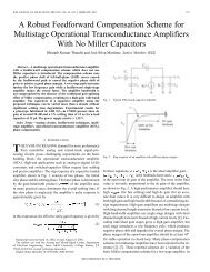
FC100%FC100%Phase IPhase IIVV(a)(b)Figure 2.7: (a) Empirical result of FC v.s V, (b) Goel's estimation.is a function of gate count (g) and nets (n).A s = as0 + as1 g 2 + as2p n (2.49)Thus, our yield model can base on poisson yield model but chip area should be replaced bythe total sensitive area (A s ). Finally, the yield model can be expressed asY = e , dA s(2.50)2.6.3 Fault CoverageFault coverage is used to estimate defect level as shown in (2.46). However, in this equation,the equiprobable faults include all possible faults. Precise analysis of all possible faultsneeds consider various fault model. However, the experience result of Ma [21] shows thateven though the single stuck-at fault may be inaccurate to model real faults, a sucienthigh single stuck-at fault coverage may be adequate to achieve high quality levels. Thus, weassume this is a high fault coverage project and target our fault coverage analysis on singlestuck-at fault model.This subsection also estimate test vector length. This parameter is mainly used to estimatethe testing cost. However, fault coverage is a function of the test length and defectlevel aected by the fault coverage. Thus, trade-o between defect level and testing cost canbe regarded as trade-o between fault coverage and test length.The empirical result of relation between fault coverage and test length is shown in Fig-29

ure 2.7(a). An equation is proposed to model the result asFC =1, e ,V (2.51)where V is test length and is equation parameter for tting various circuits. This equationis rational because fault coverage raise fast in the beginning but very slow while it near 100percent. In addition, if redundant faults are regardless, fault coverage must reach 100%whentest length go to innity.Goel proposed another method to model empirical results [22]. He use two piece ofcurve to t the results, as shown in Figure 2.7(b) one is exponential and another is linear.A threshold test length V th divides test generation into two phase. In phase I, The sameequation as our model is used for estimation. When test generation enters phase II, faultcoverage is modeled as a liner equation:FC = FC 0 + kV (2.52)Besides, Kim proposed a more exible model [5]:FC = FC 0 + ke ,V ; (2.53)and estimated value is limited between upper bound (UB) and lower bound (LB).All these models have the same problem: How to determine the parameters , k andFC 0 for our circuit when the netlist still not available? Goel proved that k is a constantform four experience, but it is obviously irrational. In fact these parameters are stronglydepend on the structure of circuit. They indicate how ease the faults to be detected. Thus,user can estimate their value from chip testability (TB). For example, we can assume theyall proportional to TB.Cheng proved that it takes at most D 2 L test length to detect a single stuck-at faultwhere D is sequential depth and L is interval loop length [23]. Although this is a upperbound of each fault. It implies that how hard the fault in circuit can be detected since testlength mainly aected by these hard to detected faults. Thus, if user have rational value ofD and L for their circuit, our parameters also can be estimated from this upper bound. Forexample, we can assume they are all inverse proportional to D 2 L .30

In our study, we run ATPG for ISCAS89 benchmark circuits to obtain relation of FCand V in Section 4.2.1. We choose (2.52) to t curve of our experience because that equationuse only one parameter . This can simple our comparison among the circuits. Then, ofthese circuit were estimated using least square curve tting algorithm.After the relation between fault coverage and test length is established, we must decidethe value of them to archive minimal cost. Kim [5] proposed to set test length at a thresholddF C=dV value [5], but fault coverage in this threshold is usually not enough. Thus, we onlysupport the procedure: User may decide test length, estimate FC, then check if DL satisfyspec, recursively.Once the test length is decided, it will be sent to time model to estimate test time. Then,test cost will be evaluated according to test time.Now, there is another problem: how to balance test length of three test stages to achieveminimal total cost. As previous discussion, the earlier defect chips are eliminated, the fewerpenalty cost of those chips is needed. Lower defect level of each test stage will reduce chipmanufacturing cost. For example, we assume wafer cost can eliminate almost all defect dies,so we don't need to pay any package cost, pre-burn-in testing cost and nal testing cost forthose defect dies. The total cost is therefore reduced. However, lower defect level meanshigher testing cost since longer test length for higher fault coverage is needed.Moore proposed a program to model testing cost of the whole system manufactured inDEC production process [24]. Then, this program determine the most economic test processwithout sacricing defect level. Their experience result shows when defects per unit (DPU)is low, the optimal test process is system test only. But in high DPU, optimal process iscompound of chip test and system test. The same idea can be used in our three test stages.When yield is high, we can reduce test length in early test stages to reduce the test cost. Incontract, while low yield, wafer test needs higher fault coverage to reduce cost of defect dies.In addition, two parameters (R wf , R pf ) are proposed as the ratio of the test length ofeach test stage. It is expressed asV w = R wf V f ;V p = R pf V p ;(2.54)where V w , V p , and V f is test length of the wafer, pre-burn-in, and nal test. As above31

explanation, when yield is high, user should set R wf and R pf to low, and vice versa.Finally, fault coverage of three test stage can be estimated asFC w =1, e , fcV w;FC p =1, e , fcV p;(2.55)2.7 Market Life ModelFC f =1, e , fcV f:We now turn to the revenue model, which is delineated in Fig. 2.8. It is well known that, ingeneral, the earlier the product is put on the market the more revenue we will receive. Therevenue R is obtained from the products sold in the market, plus other user dened revenuesuch as that from patent right or technology transfer. Fig. 2.8 shows the market life cycleforatypical product, which is the default model in our system.RevenueTTMrev_dftTTMrevTime savingTTMgrow TTMmatu TTMdeclTimeFigure 2.8: The market life cycle model.In the gure, TTM grow is the market growing period, TTM matu the market maturityperiod, TTM decl the market declining period, and TTM rev the maximal revenue. The revenueis calculated as the area covered by the curve throughout the product's market life. Thus,the revenue can be expressed asR = 1 2 (TMM grow +2TMM matu + TMM decl ) TMM rev (2.56)If the product is earlier to the market due to DFT design added, the revenue loss is calculatedas the area of the shaded region shown in the gure. Then, revenue equation should be modify32

asR dft = 1 2 (TMM grow +2TMM matu ) TMM rev Tdsave + TMM grow + TMM2matuTMM grow + TMM matu+ 1 2 TMM decl TMM rev Td save + TMM grow + TMM matuTMM grow + TMM matu;(2.57)where Td save is development time saved by DFT.Notice that TTM rev of the no-DFT product should be given by the user, and we assumethat all products in the market die at the same time.2.8 Impact of Design for TestabilityThe goal of our system is to compare the economical dierence among various test methodologies.We had construct the economic models to model cost and revenue of the design inproceeding sections. Now, we want to obtain the eect of test methodologies. As shown inPin Count Gate Count Complexity Testability Test Length Fault CoverageAreaDevelop TimeTesting TimeManufacturing Cost Developmental Cost Testing Cost YieldRevenueTotal CostProfitDevect LevelFigure 2.9: DFT impact on parameters.Figure 2.9, DFT will aect pin count, gate count, complexity, testability, etc. Then, thoseparameters will change the area, development time, testing time, etc. Finally, the eects willpropagate to prot and defect level. We can compare them to obtain which test strategy ismore suitable to this design. For now, we only list which parameters will be aected. The33

future work is to quantify those eects. In Chapter 4, we will shown our experiment of fullscan design, and obtain the change of parameters in scan design.34

Chapter 3System DevelopmentIn our study, a software system, called "Evaluation System for TEst Engineering (ES-TEEM)", has been developed. The goal of this system is to nd maximal prot test strategyin the early stage of the design.This system is intended for use by industry, because we try to collect design data fromthem for more precise models in the future. Thus, the hole system is designed to be accessedfrom Internet. User can connect to our system form arbitrary computer via web browser.Besides, the system also provide security to protect data of each user.Because the cost strongly depends on the design ow of each company, the users mustmodify equations and parameters in our models to match the condition of their companies.The design of the user interface needs to be more exible that user can easily modify theequations and parameters on line. Moreover, user can customize their own default modelequations and parameters for convenience.In the rest of this chapter, we describe details of the ESTEEM system. The systemarchitecture will be introduced in the rst section. Then, we shows the analyze ow of oursystem in the second section. The third section demos the user interface and the last sectionexplains the algorithm of the analyze engine program in our system.3.1 System ArchitectureThe architecture of the whole system is shown in Figure 3.1. Our system includes programsin server and client. Some of those programs are well-developed packages, so we just needto custom them to t our system.35

AnalyzeEngineMsqlServerSystem DataUser DataResult Display Model Editor File ManagerInterface CGIServer SideWeb ServerUser Auth DataInternetCilent SideWeb BroswerModified ModelsAnalyzed ResultsFigure 3.1: Architecture of ESTEEM.There are four programs and three databases in the server. The web server is developed byApache origination. This program handles all data owbetween server and client. Besides, italso check login account and password of each user for security. The Msql server is a databaseengine. This server is proved by Hughes and free for academics. It controls accesses to systemand user databases. Analysis engine is developed by us. This is a Perl program that guresout results from user input data. Details will be discussed in Section 3.4. Interface CGIprogram is consisted of three part: File Manager, Model Editor, and Result Display. CGI isbrief of "common gateway interface". It means that this program can handle informationsof WWW format. Our interface CGI is a complex program that integrated using Perl, Java,and Javascript programming language. We will show details in later section.User Auth Database include information of each user account. It includes login name,password, and user's personal data. System Database stores system default model equationsand parameters. This database can be accessed by any authorized user. In contrast, UserDatabase stores private data of each user. Each user can only access its own private data inthis database.In the client, user needs to run web browser to connect to our web server. We suggest"Netscape" as the browser. In addition, user have to open the promission of executing Javaand Javascript on the browser. After that, user can modify models and obtain results from36

the browser.3.2 Analysis FlowConnectLoginUser AuthDatabaseFile ManagerModel EditorSystemDatabaseAnalysis EngineResult DisplayUserDatabaseNoMeetConstrainYesFinishFigure 3.2: Analysis ow of ESTEEM.Figure 3.2 shows the ow chart of analysis process. The process starts from accessing toour server via web browser. System prompt login account and password for authorization.Then, File Manager is used to select saved projects or create new projects. After selecting,system invokes Model Editor and accesses models of the selected project form database.Test methodologies, equations, and parameters can be modied by Model Editor. Afterthat, Analysis Engine is invoked to calculate results. This results will be sent to ResultDisplay. User can check if prot and defect level meet their constrain. If they do, the jobis nished. Else, the user has to go back to Model Editor for some modication, and re-runAnalysis Engine.37

Figure 3.3: File Manager.3.3 User InterfaceThe user interface includes three programs: File Manager, Model Editor and Result Display.File Manager help user manage their projects as general les. Figure 3.3 shows the FileManager. In this program, users can create, remove, copy and open their own les anddirectories. Its operation is similar to general le managers. This program is written by Perland Javascript, because Perl is excellent in handling WWW data and Javascript can easilyproduce dynamic homepages.Once a le is opened, model editor will be invoked to read data from selected project.Thus, user can modify parameters and equations of models to match their design. Ourprevious version is written by pure Java. But, Java is restricted by it's low performance andstability. Too large Java applet will slow down the speed of browser and may lead to crash.This version is written by Perl, Java, and Javascript. Java is only used to handle someactive display that Javascript is not powerful enough to do. Figure 3.4(a) shows the appletof block parameters. It uses card layout. User can indicate how many blocks in the chip,and modify parameters of each block easily. Figure 3.4(b) shows the applet of quality model.38

(a)(b)Figure 3.4: Model Editor: (a) block parameters, (b) fault coverage and testlength.39

User can modify parameters by pulling the circle to adequate position or changing the valuesin the text eld directly.Figure 3.5: Result Display.Result Display displays results from analysis engine. This is a program written by Perland GD library. GD is a graphic library which is used for generating GIF format graph forour result pages. Figure 3.5 shows the Result Display.3.4 Program AlgorithmIn this section, we only describe the algorithm of analysis engine. This program parses eachequation and calculates value of each variable. We choose Perl as our programming languagebecause this language implements pattern match and powerful parser library.The data structure of each equation is as follow:struct equation {string *parameter;string *value;}40

If this equation is a function, for example f(x; y) =2x 2 + y, this function will be parsed tothis structure as follow: "f" is the structure name, "x; y" is the parameter and "2x 2 + y" isthe value. If this equation is just a scalar, for example C = Cm+ Cd+ Ct+ K, "C" will bethe structure name and "Cm + Cd + Ct + K" will be value. Because this kind of equationdoes not have parameters, a string "var" is stored in the parameters eld of the structure.Finally, the whole algorithm is listed as follows:calc{$equation){if($equation->value is a numerical value){return true;}else if($equation->parameters != "var")recurn false;}while($equation->value have non-numerical pattern){$pattern = extract_pattern($equation->value);if(calc($pattern)){replace $pattern to $pattern->value;} else { // this is a function$pattern_parameters = extract_fx($pattern);$fx_value = lookup_fx($pattern, $pattern_parameters);replace $pattern to $fx_value;}calculate $equation->value;}This program will recursively replace variables and functions in a equation untill the equationcontain only numerical value. Then, the value is gured out.41

Chapter 4Experimental Result4.1 ISCAS89 Benchmark OverviewThe ISCAS'89 test generation benchmark data can be obtained from ftp://mcnc.mcnc.orgor http://www.cbl.ncsu.edu/benchmarks. This benchmark suit contains a total of 31 circuitbenchmarks; their essential statistics are shown in Table 4.1 [25]. The naming conventionis similar to the ISCAS'85 set: s# The letter s signies that the circuit is synchronoussequential; the number that follows represents the number of interconnect lines among thecircuit primitives.A total of seven ISCAS'89 benchmark circuits have been modied. Four of the sevencircuits have been modied to eliminate ip-ops that were unreachable by any path startingat the primary inputs. This was accomplished by removing selected ip-ops from thecircuit and declaring these ip-op inputs and outputs to be primary outputs and inputs,respectively. The aected circuits are s9234, s13207, s15850 and s38584. The other threecircuits modied are digital fraction multipliers that were functionally incorrect. The aectedcircuits are s208, s420 and s838. All seven circuits have been renamed to add a .1 sux totheir names. For example, the corrected version of s208.bench is named s208.1.bench.4.2 Model Parameters EvaluationWe focus our experiment on fault coverage and chip area. They are represented in followingtwo subsection, respectively.42

Table 4.1: ISCAS'89 benchmark circuit characteristics.Name PIs POs D-FFs Gates Commons27 4 1 3 10s208 11 2 8 96 digital fractional multipliers based on PLD devicess298 3 6 14 119 trac light controllers based on PLD devicess344 9 11 15 160re-synthesized from s349, after removing all redundanciesin full-scan modes349 9 11 15 161 4-bit multipliers382 3 6 21 158re-synthesized from s400, after removing all redundanciesin full-scan modes386 7 7 6 159 controllers synthesized from HDLs400 3 6 21 162 trac light controllerss420 19 2 16 196 digital fractional multiplierss444 3 6 21 181 trac light controllerss510 19 7 6 211 controllers synthesized from HDLs526n 3 6 21 194s526 3 6 21 193 trac light controllerss641 35 24 19 379s713 35 23 19 393 based on PLD devicesre-synthesized from s526, after removing all redundanciesin full-scan modebased on PLD devices re-synthesized from s713, afterremoving all redundancies in full-scan modes820 18 19 5 289re-synthesized from s832, after removing all redundanciesin full-scan modes832 18 19 5 287 based on PLD devicess838 35 2 32 390 digital fractional multiplierss953 16 23 29 395 controllers synthesized from HDLs1196 14 14 18 259re-synthesized from s1238, after removing all redundanciesin full-scan modes1238 14 14 18 508 combinational circuit with randomly insert ip-opss1423 17 5 74 657s1488 8 19 6 653re-synthesized from s1494, after removing all redundanciesin full-scan modes1494 8 19 6 647 controllers synthesized from HDLs5378 35 49 179 2779s9234 19 22 228 5597 real-chip based and rely on partial scans13207 31 121 669 7951 real-chip based and rely on partial scans15850 14 87 597 9772 real-chip based and rely on partial scans35932 35 320 1728 16065s38417 28 106 1636 22179 real-chip based and rely on partial scans38584 12 278 1452 19253 real-chip based and rely on partial scan43

4.2.1 Fault CoverageFault coverage is a function of test length as discussion in Section 2.6. Now, we try to ndparameter of this function.0.90.80.7Fault Coverage (FC)0.60.50.40.30.20.10−0.10 20 40 60 80 100 120 140 160 180 200Test Vector Length (V)Figure 4.1: Experimental and approximated result of fault coverage.In our experiment, ISCAS'89 benchmark circuits are applied to a sequential ATPG, called"HITEC". The fault coverage of each test length is obtained, as shown in Figure 4.1. Then,equationFC(V )=1, e , fcV(4.1)is used to t the experimental results. This tting curve is also shown in the same gure.Least square tting algorithm are adopted to evaluate fc of the function. Because we generallyuse only high fault coverage results, our tting process eliminates those data which faultcoverage fewer than 0.7. All experimental and evaluated results are included in Appendix B,and summarized in Table 4.2.Moreover, we consider that scan is added into the circuits. ISCAS'89 SCAN circuits areapplied to a combinational ATPG tool, called "ATALANTA". Because scan test need shift44

Table 4.2: Fault coverage parameter approximation.Name PIs POs D-FFs Gates Depth fc Tt gen fc scan Tt gen scans27 4 1 3 10 - 0.1204 0 1.9800 0s208.1 11 2 8 96 - 0.2404 10640 1.0201 0.03s298 3 6 14 119 8 0.0045 3718 0.0177 0.03s344 9 11 15 160 6 0.0408 11650 0.1633 0.05s349 9 11 15 161 6 0.0536 51082 0.0309 0.02s382 3 6 21 158 11 0.0016 570781 0.0080 0.03s386 7 7 6 159 5 0.0173 19 0.0098 0.07s400 3 6 21 162 11 0.0013 77953 0.0088 0.03s444 3 6 21 181 11 0.0010 57739 0.0143 0.03s526 3 6 21 193 11 0.0009 57739 0.0037 0.08s641 35 24 19 379 6 0.0285 13 0.0054 0.11s713 35 23 19 393 6 0.0378 18 0.0054 0.18s820 18 19 5 289 4 0.0044 543 0.0070 0.15s832 18 19 5 287 4 0.0037 789 0.0068 0.20s953 16 23 29 395 - 0.2814 155 0.0020 2.03s1196 14 14 18 259 4 0.0074 2 0.0019 0.35s1238 14 14 18 508 4 0.0069 8 0.0018 0.62s1488 8 19 6 653 5 0.0075 1318 0.0056 0.28s1494 8 19 6 647 5 0.0076 678 0.0058 0.33s35932 35 320 1728 16065 35 0.0620 12669 0.0016 7245

patterns into ip-ops, the test length (V ) should be estimated as(N FF V comb if N FF < 100;V =100 V comb if N FF > 100;(4.2)where V comb is number of test vectors generated by ATALANTA, and N FF is number ofip-ops of circuits. It is assumed that multiple scan chains are used to guarantee the lengthof each scan chain never exceed 100. Thus, the number of shifts per vector is 100 insteadof N FF , if N FF> 100. Then, similar process as no scan circuit fc estimation is used tocalculate fc scan . The results are also shown in the same table. Additionally, this table liststest generation time of both scan and no scan circuits.From this table, we nd two things:☞ Scan greatly reduces test generation time. As shown in the table, circuit with no scanmay need even weeks to generate high fault coverage patterns. However, this time isreduced to almost zero in scan-added circuits.☞ Similar circuits have close fc . This result can be obtained by comparing fc of thepairs of circuits: (s382, s400), (s641, s713), (s820, s832), (s1196, s1238), and (s1488,s1494). They are synthesized from the same function as listed in Table 4.1.Another experiment is comparing random pattern and scan design. Random pattern donot need test generation time, and scan design use almost zero time to generation pattern.As shown in Table4.3, the test length of random pattern is much longer than scan design.4.2.2 AreaThe synthesized results of both scan and no scan benchmark circuits are listed in Table 4.4.This table also include evaluated result of gate area ratio (A/G). The target process isTSMC.6 DPDM process.Result of this table shows that gate area ratio is a value typically between 0.8 to 106.Moreover, scan circuit area is proportional to number of ip-ops in the circuit. The totalarea, after scan insertion, can be expressed asA scan = A +2N FF ; (4.3)where A is original circuit area, and N FF is number of ip-ops in the circuit.46

Table 4.3: Fault coverage and test length of random pattern.Name Vectors max fc scan clockss27 88 1 18s208.1 1000 1 280s298 1e7 0.93 420s344 1000 1 330s349 2000 1 345s382 1e8 0.21 210s386 1e8 0.98 483s400 1e8 0.21 651s444 1e8 0.20 672s526 1e8 0.14 1344s641 1e5 0.99 1007s713 1e5 0.99 989s820 1e8 0.56 570s832 1e8 0.57 555s953 100 1 2581s1196 1e7 1 2484s1238 1e7 1 2794s1488 1e8 0.98 744s1494 1e8 0.98 762s35932 1e5 0.97 670047

Table 4.4: Circuit area of benchmarks.Name PIs POs FFs Gates Area A/G A Scan A diff A diff /FFss27 4 1 3 10 30 3.00 36 6 2.0s298 3 6 14 119 187 1.57 215 27 1.9s344 9 11 15 160 216 1.35 246 30 2.0s349 9 11 15 161 219 1.36 249 30 2.0s382 3 6 21 158 267 1.68 309 42 2.0s386 7 7 6 159 145 0.91 157 12 2.0s400 3 6 21 162 265 1.63 308 43 2.0s420 19 2 16 196 236 1.20 269 12 2.1s444 3 6 21 181 265 1.46 307 43 2.0s510 19 7 6 211 257 1.21 269 12 2.0s526n 3 6 21 194 304 1.56 346 42 2.0s526 3 6 21 193 297 1.54 340 43 2.0s641 35 24 19 379 255 0.67 293 38 2.0s713 35 23 19 393 253 0.64 292 39 2.1s820 18 19 5 289 283 0.98 293 10 2.0s832 18 19 5 287 284 0.99 294 10 2.0s838 35 2 32 390 480 1.23 545 65 2.0s953 16 23 29 395 526 1.33 584 58 2.0s1196 14 14 18 259 572 2.21 608 32 2.0s1238 14 14 18 508 580 1.14 616 36 2.0s1423 17 5 74 657 992 1.51 1141 149 2.0s1488 8 19 6 653 567 0.86 579 12 2.0s1494 8 19 6 647 569 0.88 581 12 2.0s5378 35 49 179 2779 2305 0.83 2665 360 2.0s9234 19 22 228 5597 2961 0.53 3385 1424 2.1s13207 31 121 669 7951 6545 0.82 7829 1284 1.9s15850 14 87 597 9772 6561 0.67 7635 1074 1.8s35932 35 320 1728 16065 21038 1.31 24517 3479 2.1s38417 28 106 1636 22179 19733 0.88 23028 3295 2.0s38584 12 278 1452 19253 20421 1.06 23292 2871 2.048

4.3 Case StudyIn this section, a real case of IEEE 1149.5 MTM-bus slave module [9] is used to analysis.Figure 4.2 shows the overall architecture of this chip. We describe the parameters requiredBlock 1 Block 2 Block 3 Block 4AddressComparatorCommandDecoderPacketCounterIEEE 1149.5ReceiverAddressPacketAddress 8 2 Command 7 1216ModeControlNumber1IPCMCLKMCTLMMD1MSD_sysMSD16411117Echo DataIEEE 1149.5Transmitter5511ControlSignalRegister&ControllerBlock 616SignatureModuleRegister39 Status16TMS Data&Test PatternIEEE1149.1Data TransferPort44144TCKTMSTRSTTDITDOBlock 5Block 7Figure 4.2: Architecture of IEEE 1149.5 MTM-bus slave module.by our analysis from Table 4.5 to 4.10.Table 4.5: Parameters of chip.Chip level parameters Notation no-DFT DFTchip area A 11.2 12.3 mm 2chip gates G 11136 12249chip nets N 16314 17945chip pins P 48 52chip testability TB 0.3 0.55chip complexity , 0.8 0.96After applying all parameters to the system, we invoke the analysis engine and get resultswhich is shown in Table 4.11. The results include value of with and without DFT. As shown49

Table 4.6: Parameters of each block.block type gates nets I/Os gar nar tb1 logic 659 742 84 0.8 0.1 1e-3 3e-5 0.32 logic 624 924 10 0.8 0.1 1e-3 3e-5 0.33 logic 2192 2802 19 0.8 0.1 1e-3 3e-5 0.34 logic 2731 4021 17 0.8 0.1 1e-3 3e-5 0.35 logic 1512 2202 73 0.8 0.1 1e-3 3e-5 0.36 logic 2053 3803 14 0.8 0.1 1e-3 3e-5 0.37 logic 1365 1820 49 0.8 0.1 1e-3 3e-5 0.3Table 4.7: Parameters in cost model.Cost Model parameters notation valuesalary of Manager Ud mang 120000 ntmanagement time ratio Rd mang 0.2salary of each engineer Ud eng 40000 ntnumber of engineers Nd eng 1design hardware cost Cd hw 200000 ntdesign hardware depreciative rate Rd hw 0.02design software cost Cd sw 100000 ntdesign software depreciative rate Rd sw 0.02cost per prototyping C proto 1000000 ntnumber of prototyping N proto 3cost per wafer U wafer 100000 ntwafer radius R w 150 mmutilization of wafer R wutil 0.9cost of mask C mask 1000000 ntpackage cost parameter U p 10package cost parameter U pp 0.08wafer test equipment cost Ctw eq 200M ntequipment depreciative rate Rtw eq 0.4equipment maintenance cost Ctw mt 500K ntnumber of equipment test pins Ptw eq 256pre-burn-in test equipment cost Ctp eq 200M ntequipment depreciative rate Rtp eq 0.4equipment maintenance cost Ctp mt 100K ntnumber of equipment test pins Ptp eq 256nal test equipment cost Ctb eq 200M ntequipment depreciative rate Rtb eq 0.4equipment maintenance cost Ctb mt 1M ntnumber of equipment test pins Ptb eq 25650

Table 4.8: Parameters of time model.Time model parameters Notation Valuechip development time dG 0.0003block development time dg 0.0001wafer testing time tw 0.0006pre-burn-in testing time tw 0.0002nal testing time tw 0.0002Table 4.9: Parameters of market life model.market life model parameters Notation Valuemaximal revenue per month M r 3000000 ntmarket growing period M g 6 monthmarket maturity period M m 8 monthmarket decline period M d 2 monthTable 4.10: Parameters of quality model.Quality model parameters Notation Valuesensitive area as0 0.01sensitive area as1 5e-8sensitive area as2 8e-10defect density d 0.002 pots=mm 2wafer and nal test length ratio Rwb 0.3pre-burn-in and nal test length ratio Rpb 0.3fault coverage fc 1e-5burn-in test length Vb 400K51

Table 4.11: Result of analysis.Analysis result Notation no-DFT DFTprot prof 29.7M 38.8M nttotal cost cost 6.33M 6.26M nttotal cost per chip C 551 546 ntdevelopment cost Cd 370 361 ntmanufacturing cost Cm 153 158 nttesting cost Ct 27 27 ntdevelopment time Td 14 12 monthwafer test time Ttw 72 64 secondpre-burn-in test time Ttp 76 68 secondnal test time Ttb 80 72 secondrevenue R 36M 45M ntyield Y 0.9987 0.9851fault coverage FC 0.982 0.999defect level DL 227 11 DPMin this table, DFT will reduce the development time by 2 months, so the revenue increasesfrom 36M to 45M. The prot increases from 29.7M to 38.8M. Moreover, DFT increases area,so the yield reduces from 0.9987 to 0.9851. However, DFT increases fault coverage from0.982 to 0.999. The defect level reduces from 277 to 11 DPM. In this case, DFT increaseboth prot and quality.After that, we analysis the cost of dierent volume. As shown in Table 4.12, we comparecost for volume from 10k to 320k. Cd, Cm, and Ct are development, manufacturing, andtesting cost of no-DFT. C is total cost without DFT. Cd dft , Cm dft , Ct dft , and C dft are thecost with DFT. By comparing value of each stage cost with and without DFT, we can ndthat DFT decreases development and testing cost, but it increases manufacturing cost. Thus,as shown in last two column, DFT may not reduce the total cost when the volume is high.To analysis the case of larger chip, we multiply gate count of each block by ten. The costof this case is shown in Table 4.13. As shown in last two column, the total cost with DFTis higher than design without DFT, when the volume is high.Figure 4.3 shows the bar chart of cost and volume. By this chart, we can nd thethreshold volume 80K. We get benet form DFT, if the volume lower this threshold.To see why cost of DFT will not get benet any more, the cost ratio of each stage is shown52

Table 4.12: Cost of dierent volume.Nv Cd Cd dft Cm Cm dft Ct Ct dft C C dft10K 370 361 153 158 109 106 633 62620K 185 180 103 108 109 106 398 39530K 123 120 87 91 109 106 319 31840K 92 90 78 83 109 106 280 28060K 61 60 70 74 109 106 241 241Table 4.13: Cost of dierent volume in larger area case.Nv Cd Cd dft Cm Cm dft Ct Ct dft C C dft10K 1711 1199 594 655 256 253 2562 211720K 855 599 544 615 256 253 1656 146740K 427 299 519 590 256 253 1203 114280K 213 149 506 577 256 253 976 980160K 106 74 500 571 256 253 863 898320K 53 37 497 568 256 253 807 858Cost26002400220020001800NoDFTDFT160014001200100080060010K 20K 40K 80K 160K320KVolumeFigure 4.3: Relation between cost and volume.53

(a)(b)Figure 4.4: Stage cost ratio of 2k volume: (a) Original, (b) DFT.(a)(b)Figure 4.5: Stage cost ratio of 320k volume: (a) Original, (b) DFT.54

in Figure 4.4 for 2K volume and Figure 4.5 for 320K volume. DFT greatly reduces developmentcost, but increases manufacturing cost. However, development cost is no-recurrentcost. It has low ratio in high volume. Manufacturing cost mainly consists of recurrent cost.This cost will dominate total cost in high volume. Thus, the total cost of DFT will higherthan no-DFT case.55

Chapter 5ConclusionsWe have shown that if we select suitable test strategy for the design, the prot will greatlyincrease. Economic models had been developed to help nd the optimal test strategy. Weproposed four economic models, a set of circuit parameters, and a test methodologies library.Base on the previous works, a quality model had been added to provide more accurateestimation value of test related parameters, such as fault coverage, yield and defect level.The whole system now includes four models: Cost Model, Time Model, Quality Model andMarket Life Model. Cost Model estimates the total cost and Market Life Model estimatesthe revenue. Moreover, Time Model estimate the time related parameters. Besides, in thecircuit description, many suggestion and heuristics have been proposed to help estimatecircuit parameters which are hard to obtain.In the system, the new version of ESTEEM provides more security for users data. Thesystem uses Perl, Java and Javascript languages and integrates web server, SQL server, andCGI programs. This system provides more friendly users interface, such as le manager,model editor, and result display. Besides, a more powerful analysis engine had been developed,so user can easily add new equations or modify proposed models to t the conditionof their companies.In addition, we had done some experiments to obtain eects of scan design. The ISCAS'89benchmark circuits were applied to sequential ATPG and random pattern fault simulatorto nd the relation between fault coverage and test length. Then, ISCAS'89 SCAN circuitswere applied to combinational ATPG to obtain similar relation. The relation of three designmethods: sequential ATPG, random pattern, and scan were compared. Moreover, ISCAS'8956

circuits were translated to Verilog format for synthesis. The synthesized area of ISCAS'89and its scan version were compared, too.Finally, an IEEE 1149.5 MTM-Bus slave module chip is analyzed by our system. Theresult shows that the DFT prot will greatly increase if DFT is used, since it saves thedevelopment time and shortens time to market. Besides, by comparing dierent volumes forthe same case, we found a threshold volume. The total cost with DFT is lower than thatwithout DFT under this threshold volume.This is an on-going project, where modeling the eect of more test methodologies, performanceimpact of DFT, more realist models developed from the collected data will be donein the future. Beside, optimization and auto learning capability will be investigated.57

Appendix ASummary of All ModelA.1 Cost ModelC = Cd + Cm + Ct + K(Eq.2.9, pp.16)A.1.1Developmental costCd = C dsgn + Cd mang + Kd(Eq.2.23, pp.20)Design CostC dsgn = Cd mp + Cd equip + Cd space + C proto + K dsgn(Eq.2.24, pp.20)Design man-power cost:Cd mp = Ud eng Nd eng T dsgn + Kd mp(Eq.2.25, pp.21)Design equipment cost:Cd equip =Xf dp (R dp )=1, (1 , R dp ) T d(Eq.2.27, pp.22)U hw f dp (R hw dp )+U hw mt T d + C hw traineach Xhw (Eq.2.28, pp.22)+U sw f dp (R sw dp )+U sw mt ) T d + C sw traineach swOr use Type II cost model:XCd equip =(U hw R hw dp + U hw mt ) T d + C hw traineach Xhw (Eq.2.29, pp.22)+(U sw R sw dp + U sw mt ) T d + C sw traineach sw58

Design space cost for rent building companies:Cd space = Rd space U rent T d + K space(Eq.2.30, pp.22)For buy building companies:Cd space = Rd space U space [(1 + R int ) T d, (1 + R sp ap ) T d]+K space(Eq.2.31, pp.22)Prototypes cost for fab prototyping:C proto = N proto U mask + K proto(Eq.2.33, pp.23)For FPGA and emulator prototyping, cost implied in equipment cost.Management CostCd mang =Xper manager(U mang R mang T d )+Kd mang (Eq.2.34, pp.23)A.1.2Manufacturing CostCm = C mask =N v + U die + U pack + Km(Eq.2.35, pp.24)Cost per die:Package cost per chip:U die = U wafer =n g = 4AU wafer util d 2 YU pack = p + pp P(Eq.2.37, pp.24)(Eq.2.38, pp.24)A.1.3Testing CostWafer test cost:Ct w = Xper tw eqPre-burn-in test cost:Ct p =Final test cost:Ct f = Xper tp eq Xper tf eqCt = Ct w + Ct p + Ct f + Kt;Ct w eq Rt w eq + Ct w mtP Tt w =Y + Kt w ;Pt w eqCt p eq Rt p eq + Ct p mtP Tt p + Kt p ;Pt p eqCt f eq Rt f eq + Ct f mtP Tt f + Kt f ;Pt f eq(Eq.2.39, pp.24)(Eq.2.41, pp.25)(Eq.2.42, pp.25)(Eq.2.43, pp.25)59

A.2 Time ModelDevelop time:T d = e td GG,(1,TB) +Xper blocke td gg(1,)(1,tb) :(Eq.2.44, pp.27)Testing time:Tt w = tw V w ;Tt p = tp V p ;Tt f = tb V f ;(Eq.2.45, pp.27)A.3 Quality ModelDefect level:DL w =1, Y 1,FCwDL p =1, Y 1,FCpDL f =1, Y 1,FC f;(Eq.2.47, pp.28)Total sensitive area:A s = as0 + as1 g 2 + as2p n(Eq.2.49, pp.29)Yield:Y = e , dA s(Eq.2.50, pp.29)Test length:V w = R wf V fV p = R pf V p ;(Eq.2.54, pp.31)Fault coverage:FC w =1, e , fcV wFC p =1, e , fcV p(Eq.2.55, pp.32)A.4 Market Life ModelRevenue of no-DFT design:FC f =1, e , fcV fR = 1 2 (TMM grow +2TMM matu + TMM decl ) TMM rev(Eq.2.56, pp.32)60

Revenue with DFT design:R dft = 1 22 (TMM grow +2TMM matu ) TMM rev Tdsave + TMM grow + TMM matuTMM grow + TMM matu+ 1 2 TMM decl TMM rev Td save + TMM grow + TMM matuTMM grow + TMM matu;(Eq.2.57, pp.33)61

Appendix BFault Coverage Approximation ofISCAS'89 Benchmarks27s208.10.90.90.80.80.70.7Fault Coverage (FC)0.60.50.40.3Fault Coverage (FC)0.60.50.40.30.20.20.10.100−0.10 2 4 6 8 10 12 14 16 18 20Test Vector Length (V)PIs 4 Vectors 21POs 1 fc 0.1204FFs 3 Err Sqrt 1.2e-3Gates 10−0.10 2 4 6 8 10 12Test Vector Length (V)PIs 11 Vectors 12POs 2 fc 0.2404FFs 8 Err Sqrt 1.8e-3Gates 9662

1s298s344Fault Coverage (FC)0.90.80.70.60.50.40.30.2Fault Coverage (FC)0.90.80.70.60.50.40.30.20.10.1000 20 40 60 80 100 120 140 160 180 200 220Test Vector Length (V)PIs 3 VectorsPOs 6 fc 0.023FFs 14 Err Sqrt 4.5e-3Gates 119Depth 8−0.10 20 40 60 80 100Test Vector Length (V)PIs 9 Vectors 115POs 11 fc 0.0408FFs 15 Err Sqrt 2.1e-4Gates 160Depth 6s349s3820.90.90.80.80.70.7Fault Coverage (FC)0.60.50.40.3Fault Coverage (FC)0.60.50.40.30.20.20.10.100−0.10 20 40 60 80 100Test Vector Length (V)PIs 9 Vectors 113POs 11 fc 0.0536FFs 15 Err Sqrt 2e-3Gates 161Depth 6−0.10 500 1000 1500 2000Test Vector Length (V)PIs 3 Vectors 2352POs 6 fc 0.0016FFs 21 Err Sqrt 2e-3Gates 158Depth 1163

s386s4000.90.90.80.80.70.7Fault Coverage (FC)0.60.50.40.3Fault Coverage (FC)0.60.50.40.30.20.20.10.100−0.10 50 100 150 200 250Test Vector Length (V)PIs 7 Vectors 273POs 7 fc 0.0173FFs 6 Err Sqrt 1.9e-3Gates 159Depth 5−0.10 500 1000 1500 2000 2500Test Vector Length (V)PIs 3 Vectors 1917POs 6 fc 0.0013FFs 21 Err Sqrt 4.5e-3Gates 162Depth 11s4441*s526Fault Coverage (FC)0.90.80.70.60.50.40.30.20.10Fault Coverage (FC)0.90.80.70.60.50.40.30.20.1−0.10 500 1000 1500 2000Test Vector Length (V)PIs 3 Vectors 2497POs 6 fc 0.0011FFs 21 Err Sqrt 1.7e-3Gates 181Depth 1100 500 1000 1500 2000Test Vector Length (V)PIs 3 Max. Vec 2302POs 6 Max. FC 0.69FFs 21 fc 0.0009Gates 193 Err Sqrt 1.8e-2Depth 1164

Fault Coverage (FC)10.90.80.70.60.50.40.30.2*s526nFault Coverage (FC)0.90.80.70.60.50.40.30.20.1s6410.100 200 400 600 800 1000 1200 1400 1600 1800Test Vector Length (V)PIs 3 Max. Vec 1814POs 6 Max. FC 0.69FFs 21 fc 0.0025Gates 194 Err Sqrt 2.8e-20−0.10 20 40 60 80 100 120 140 160 180 200Test Vector Length (V)PIs 35 Vectors 203POs 24 fc 0.0285FFs 19 Err Sqrt 9e-4Gates 379Depth 6s713s8200.90.90.80.80.70.7Fault Coverage (FC)0.60.50.40.3Fault Coverage (FC)0.60.50.40.30.20.20.10.100−0.10 20 40 60 80 100 120 140 160 180Test Vector Length (V)PIs 35 Vectors 196POs 23 fc 0.0378FFs 19 Err Sqrt 3.5e-3Gates 393Depth 6−0.10 200 400 600 800 1000Test Vector Length (V)PIs 18 Vectors 1117POs 19 fc 0.0044FFs 5 Err Sqrt 7.3e-4Gates 289Depth 465

1s8321s11960.90.90.80.80.70.7Fault Coverage (FC)0.60.50.4Fault Coverage (FC)0.60.50.40.30.30.20.20.10.100 200 400 600 800 1000 1200Test Vector Length (V)PIs 18 Vectors 1136POs 19 fc 0.0037FFs 5 Err Sqrt 1.1e-4Gates 287Depth 400 50 100 150 200 250 300 350 400Test Vector Length (V)PIs 14 Vectors 439POs 14 fc 0.0074FFs 18 Err Sqrt 7.2e-4Gates 259Depth 4s1238s1488110.90.90.80.80.70.7Fault Coverage (FC)0.60.50.4Fault Coverage (FC)0.60.50.40.30.30.20.20.10.100 50 100 150 200 250 300 350 400 450Test Vector Length (V)PIs 14 Vectors 472POs 14 fc 0.0069FFs 18 Err Sqrt 7.7e-4Gates 508Depth 400 200 400 600 800 1000Test Vector Length (V)PIs 8 Vectors 1151POs 19 fc 0.0075FFs 6 Err Sqrt 4.8e-3Gates 653Depth 566

Fault Coverage (FC)10.90.80.70.60.50.40.30.20.1s149400 200 400 600 800 1000Test Vector Length (V)PIs 8 Vectors 1107POs 19 fc 0.0076FFs 6 Err Sqrt 1.1e-3Gates 647Depth 5Fault Coverage (FC)10.90.80.70.60.50.40.30.20.1*s142300 20 40 60 80 100 120Test Vector Length (V)PIs 17 Max. Vec 122POs 5 Max. FC 0.45FFs 74 fc 0.0061Gates 657 Err Sqrt 2.3e-31*s53781*s132070.90.90.80.80.70.7Fault Coverage (FC)0.60.50.4Fault Coverage (FC)0.60.50.40.30.30.20.20.10.100 100 200 300 400 500 600 700 800Test Vector Length (V)PIs 35 Max. Vec 856POs 49 Max. FC 0.73FFs 179 fc 0.0028Gates 5597 Err Sqrt 2.0e-200 20 40 60 80 100 120 140 160 180 200Test Vector Length (V)PIs 31 Max. Vec 182POs 121 Max. FC 0.57FFs 669 fc 0.0071Gates 7951 Err Sqrt 1.9e-267

1*s13207.11*s15850.10.90.90.80.80.70.7Fault Coverage (FC)0.60.50.4Fault Coverage (FC)0.60.50.40.30.30.20.20.10.100 50 100 150 200 250Test Vector Length (V)PIs 31 Max. Vec 5989POs 121 Max. FC 0.54FFs 669 fc 0.0047Gates 7951 Err Sqrt 3.0e-200 500 1000 1500 2000 2500 3000 3500Test Vector Length (V)PIs 14 Max. Vec 3561POs 87 Max. FC 0.45FFs 597 fc 0.00026Gates 9772 Err Sqrt 1.2e-2Fault Coverage (FC)10.90.80.70.60.50.40.30.20.1s3593200 50 100 150 200 250Test Vector Length (V)PIs 35 Vectors 374POs 320 fc 0.0622FFs 1728 Err Sqrt 1.7e-4Gates 16065Depth 35Fault Coverage (FC)10.90.80.70.60.50.40.30.20.1*s3858400 200 400 600 800 1000 1200 1400 1600 1800 2000Test Vector Length (V)PIs 12 Max. Vec 2079POs 278 Max. FC 0.30FFs 1452 fc 0.00024Gates 19253 Err Sqrt 8.7e-368

1*s38584.10.90.80.7Fault Coverage (FC)0.60.50.40.30.20.100 1000 2000 3000 4000 5000 6000 7000Test Vector Length (V)PIs 12 Max. Vec 7914POs 278 Max. FC 0.72FFs 1452 fc 0.00026Gates 19253 Err Sqrt 2.5e-169

List of Parameters,: chip complexity.....................11 p : package cost parameter . ...........24 as0 : total sensivitve parameter 0 ......29 as1 : total sensivitve parameter 1 ......29 as2 : total sensivitve parameter 2 ......29 fc : fault coverage estimation parameter32 pp : package cost parameter ...........24 td G :chip development time parameter27 td g : block development time parameter27 tf : nal test time and length ratio . . . . 27 tp : pre-burn-in test time and length ratio27 tw : wafer test time and length ratio . . . 27 util : utilization of wafer . ..............24: block complexity....................13: block reusability....................13 d : defect density......................29A: chip area ...........................12a: block area. . . ........................11A p : area per pad.......................12A s : total sensitive area.................29C: total cost .......................15, 16C dsgn : design cost . . . ...................20C hw train : trainning cost of designhardware ......................22C mask : mask cost ......................24C proto : prototype cost . . . ...........20, 23C space : design space cost ...............22C sw train : trainning cost of design software................................22Cd: development cost . . ............16, 20Cd equip : design equipment cost . ....20, 22Cd mang : design management cost . . . 20, 23Cd mp : design man-power cost ......20, 21Cd space : design space cost ..............20Cm: manufacturing cost . . .........16, 24Ct: testing cost . ...................16, 24Ct f : burn-in test cost ..................25Ct f : nal test cost .....................24Ct p : pre-burn-in test cost ..........24, 25Ct w : wafer test cost................24, 25Ct f eq : price of nal test equipment....25Ct f mt : maintenance cost of nal testequipment.....................25Ct p eq : price of pre-burn-in test equipment25Ct p mt : maintenance cost of pre-burn-intest equipment.................25Ct w eq : price of wafer test equipment...25Ct w mt : maintenance cost of wafer testequipment.....................25d: wafer diameter . .....................24DL f : nal test defect level.............28DL p : pre-burn-in test defect level......28DL w : wafer test defect level............28f dp : depreciative dierence ratio function22FC f : nal test fault coverage. . . ....28, 32FC p : pre-burn-in test fault coverage28, 32FC w : wafer test fault coverage . ....28, 32G: gate count of chip..................11g: gate count of block..................10gar: gate area ratio of block...........10K: user dened total cost ..............16K dsgn : user dened design cost . . . . .....20K proto : user dened prototype cost .....23K space : user-dened space cost .........22Kd: user dened development cost .....20Kd mang : user dened mangement cost. .2370

Kd mp : user-dened man-power cost . . . . 21Km: user dened manufacturing cost . . 24Kt: user dened testing cost...........24Kt f : user dened nal test time .......25Kt p : user dened pre-burn-in test time.25Kt w : user dened wafer test time . .....25n: number of nets in block.............10N B :number of blocks in chip...........9N proto : number of prototyping rounds . . 23nar: net area ratio of block............11Nd eng :number of design engineers . ....21P :chip pins. .......................12, 24p: number of I/Os of block.............10Prof: prot . ..........................15Pt f eq :number of test pins of nal testequipment.....................25Pt p eq : number of test pins of pre-burn-intest equipment.................25Pt w eq :number of test pins of wafer testequipment.....................25R: revenue.........................15, 32R hw dp : depreciative rate of designhardware ......................22R mang : management man-power timeratio . ..........................23R pf : pre-burn-in and nal test lengthratio . ..........................31R space : design department space ratio . . 22R sw dp : depreciative rate of designsoftware . .....................22R wf : wafer and nal test length ratio . . 31Rd sp ap : appreciative rate of space .....22Rt f eq : depreciative ratio of nal testequipment.....................25Rt p eq : depreciative ratio of pre-burn-intest equipment.................25Rt w eq : depreciative ratio of wafer testequipment.....................25tb: block testability....................13Td save : DFT saving development time. .33tm: test methodologies of block........10TMM decl : market declining period . 32, 33TMM grow : market growing period. .32, 33TMM matu : market maturity period 32, 33TMM rev : maximal revenue.........32, 33Tt f : nal test time . ................25, 27Tt p : pre-burn-in test time . . . .......25, 27Tt w :wafer test time. ...............25, 27U die : cost per die.......................24U hw mt : maintainence cost of designhardware......................22U hw : price of design hardware..........22U mang : salary of manager ..............23U pack : package cost of each chip........24U proto : prototyping cost per round. . . . . .23U rent : annual rent......................22U sw mt : maintainence cost of designsoftware.......................22U sw : price of design software...........22U wafer : cost per wafer..................24Ud eng : average salary of engineers . . ....21V f : nal test length of chip.....14, 31, 32v f : nal test length of block...........14V p : pre-burn-in test length of chip . 14, 31,32v p : pre-burn-in test length of block.....14V w :wafer test length of chip....14, 31, 32v w : wafer test length of block..........14Y : yield . .......................24, 28, 29t: type of block.........................9T d : development time . .................27T dsgn : design time. .....................21TB:chip testability....................1471

Bibliography[1] M. Abramovici, M. A. Breuer, and A. D. Friedman, Digital Systems Testing and TestableDesign. New York: Computer Science Press, 1990.[2] M. S. Abadir, \TIGER: Testability insertion guidance expert system," in Proc. IEEEInt. Conf. Computer-Aided Design (ICCAD), pp. 562{565, 1989.[3] B. Davis, The Economics of Automatic Testing. London: McGraw-Hill, second ed.,1994.[4] I. D. Dear, C. Dislis, A. P. Ambler, and J. Dick, \Economic eects in design and test,"IEEE Design & Test of Computers, vol. 8, no. 4, pp. 64{77, 1991.[5] V.-K. Kim, T. Chen, and M. Tegetho, \ASIC manufacturing test cost prediction atearly design stage," in Proc. Int. Test Conf. (ITC), 1997.[6] S. Wei, P. K. Nag, R. D. Blanton, A. Gattiker, and W. Maly, \To DFT or not to DFT?,"in Proc. Int. Test Conf. (ITC), 1997.[7] C.-C. Wei, \A WWW-based VLSI test strategy analysis system," Master's Thesis, Departmentof Elec. Eng., National Tsing Hua Univ., Hsinchu, Taiwan, June 1997.[8] C.-C. Cheng, \An economic analysis system for VLSI test strategy planning," Master'sThesis, Department of Electrical Engineering, National Tsing Hua University, Hsinchu,Taiwan, June 1996.[9] C.-H. Tsai, \IEEE Std 1149.5 MTM-Bus Slave module chip design and its applicationto hierarchical system test," Master's Thesis, Department of Electrical Engineerig,National Tsing Hua University, Hsinchu, Taiwan, June 1996.[10] S. DasGupta, \Design for Test (DFT) Workshop, Methods and Cost Parameters Report,"Tech. Transfer 95113029B-TR, SEMATECH, 2706 Montoplis Drive, Austin, TX7841, Sept. 1996. http://www.sematech.org.[11] J. Grason, \TMEAS|a testability measurement program," in Proc. IEEE/ACM DesignAutomation Conf. (DAC), pp. 156{161, 1979.[12] L. H. Goldstein, \Controllability/observability analysis for digital circuits," IEEE Trans.Circuits and Systems, vol. 26, pp. 685{693, Sept. 1979.72

[13] R. G. Bennetts, C. M. Maunder, and G. D. Robinson, \CAMELOT: a computer-aidedmeasure for logic testability," IEE Proc. Pt. E, vol. 128, no. 5, pp. 177{189, 1981.[14] C. Chen and P. Menon, \An approach to functional level testabilty analysis," in Proc.Int. Test Conf. (ITC), pp. 373{380, 1989.[15] C.-H. Chen and S. Daniel G, \A novel behavioral testability measure," IEEE Tran.on Computer-Aided Design on Integrated Circuits and Systems, vol. 12, pp. 1960{1970,Dec. 1993.[16] T. W. Williams and N. C. Brown, \Defect level as a function of fault coverage," IEEETrans. Comput., vol. C-30, pp. 987{988, Dec. 1981.[17] J. T. de Sousa, F. M. Goncalves, C. M. J. Paulo Teixeira, F. Corsi, and T. W. Williams,\Defect level evaluation in an ic design environment," IEEE Trans. Circuits and Systems,vol. 15, pp. 1286{1293, Oct. 1996.[18] J. Cunningham, \The use and evaluation of yield modelsin integrated circuit manufacturing,"IEEE Trans. Semiconductor Manufacturing, vol. 3, pp. 60{71, May 1990.[19] S. Domer, S. Foertsch, and G. Raskin, \Model for yield and manufacturing prediction onVLSI designs for advanced technologies, mixed circuitry, and memories," IEEE Journalof Solid-State Circuit, vol. 30, pp. 286{294, Mar. 1995.[20] V. Kim, M. Tegetho, and T. Chen, \ASIC yield estimation at early design cycle," inProc. Int. Test Conf. (ITC), pp. 590{594, 1996.[21] S. C. Ma, P. Franco, and E. J. McCluskey, \An experimental chip to evaluate testtechniques experiment results," in Proc. Int. Test Conf. (ITC), pp. 663{672, 1995.[22] P. Goel, \Test generation costs analysis and projections," in Proc. IEEE/ACM DesignAutomation Conf. (DAC), pp. 77{84, 1980.[23] K.-T. Cheng and W. D. Agrawal, \A partical scan method for sequential circuits withfeedback," IEEE trans. comput., vol. 39, pp. 544{548, Apr. 1990.[24] T. J. Moore, \A test process optimization and cost modeling tool," in Proc. Int. TestConf. (ITC), pp. 103{110, 1994.[25] F. Brglez, D. Bryan, and K. Kozminski, \Combinational proles of sequential benchmarkcircuits," in Proc. IEEE Int. Symp. Circuits and Systems (ISCAS), pp. 1929{1934,1989.73