Introduction to Scilab - Projects

1 OverviewScilab is a programming language associated with a rich collection of numericalalgorithms covering many aspects of scientific computing problems.From the software point of view, Scilab is an interpreted language. This generallyallows to get faster development processes, because the user directly accesses to ahigh level language, with a rich set of features provided by the library. The Scilablanguage is meant to be extended so that user-defined data types can be definedwith possibly overloaded operations. Scilab users can develop their own moduleso that they can solve their particular problems. The Scilab language allows todynamically compile and link other languages such as Fortran and C: this way,external libraries can be used as if they were a part of Scilab built-in features.Scilab also interfaces LabVIEW, a platform and development environment for avisual programming language from National Instruments.From the license point of view, Scilab is a free software in the sense that theuser does not pay for it and Scilab is an open source software, provided under theCecill license [2]. The software is distributed with source code, so that the user hasan access to Scilab most internal aspects. Most of the time, the user downloads andinstalls, a binary version of Scilab since the Scilab consortium provides Windows,Linux and Mac OS executable versions. An online help is provided in many locallanguages.From a scientific point of view, Scilab comes with many features. At the verybeginning of Scilab, features were focused on linear algebra. But, rapidly, the numberof features extended to cover many areas of scientific computing. The following is ashort list of its capabilities:• Linear algebra, sparse matrices,• Polynomials and rational functions,• Interpolation, approximation,• Linear, quadratic and non linear optimization,• Ordinary Differential Equation solver and Differential Algebraic Equationssolver,• Classic and robust control, Linear Matrix Inequality optimization,• Differentiable and non-differentiable optimization,• Signal processing,• Statistics.Scilab provides many graphics features, including a set of plotting functions,which allow to create 2D and 3D plots as well as user interfaces. The Xcos environmentprovides an hybrid dynamic systems modeler and simulator.4

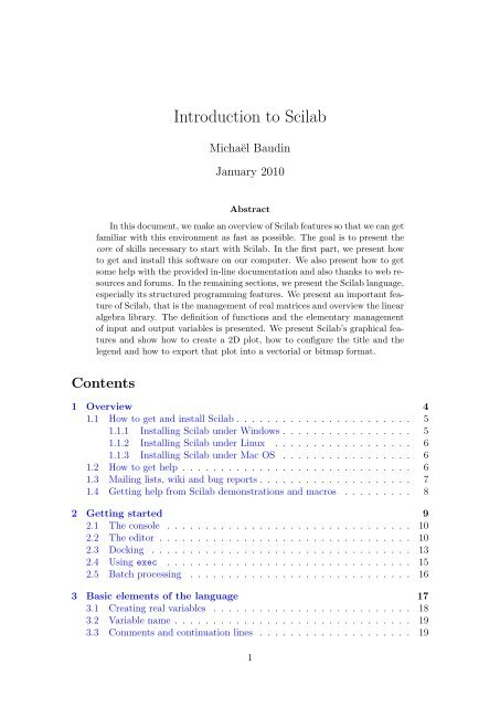
Figure 1: Scilab console under Windows.1.1 How to get and install ScilabWhatever your platform is (i.e. Windows, Linux or Mac), Scilab binaries can bedownloaded directly from the Scilab homepageor from the Download areahttp://www.scilab.orghttp://www.scilab.org/downloadScilab binaries are provided for both 32 and 64 bits platforms so that it matchesthe target installation machine.Scilab can also be downloaded in source form, so that you can compile Scilab byyourself and produce your own binary. Compiling Scilab and generating a binary isespecially interesting when we want to understand or debug an existing feature, orwhen we want to add a new feature. To compile Scilab, some prerequisites binaryfiles are necessary, which are also provided in the Download center. Moreover, aFortran and a C compiler are required. Compiling Scilab is a process which will notbe detailed further in this document, because this chapter is mainly devoted to theexternal behavior of Scilab.1.1.1 Installing Scilab under WindowsScilab is distributed as a Windows binary and an installer is provided so that theinstallation is really easy. The Scilab console is presented in figure 1. Several commentsmay be done about this installation process.On Windows, if your machine is based on an Intel processor, the Intel MathKernel Library (MKL) [4] enables Scilab to perform faster numerical computations.5

1.1.2 Installing Scilab under LinuxUnder Linux, the binary versions are available from Scilab website as .tar.gz files.There is no need for an installation program with Scilab under Linux: simply unzipthe file in one target directory. Once done, the binary file is located in /scilab-5.2.0/bin/scilab. When this script is executed, the console immediately appears andlooks exactly the same as on Windows.Notice that Scilab is also distributed with the packaging system available withLinux distributions based on Debian (for example, Ubuntu). That installationmethod is extremely simple and efficient. Nevertheless, it has one little drawback:the version of Scilab packaged for your Linux distribution may not be up-to-date.This is because there is some delay (from several weeks to several months) betweenthe availability of an up-to-date version of Scilab under Linux and its release inLinux distributions.For now, Scilab comes on Linux with a linear algebra library which is optimizedand guarantees portability. Under Linux, Scilab does not come with a binary versionof ATLAS [1], so that linear algebra is a little slower for that platform.1.1.3 Installing Scilab under Mac OSUnder Mac OS, the binary versions are available from Scilab website as a .dmg file.This binary works for Mac OS versions starting from version 10.5. It uses the MacOS installer, which provides a classical installation process. Scilab is not availableon Power PC systems.Scilab version 5.2 for Mac OS comes with a Tcl / Tk library which is disabled fortechnical reasons. As a consequence, there are some small limitations on the use ofScilab on this platform. For example, the Scilab / Tcl interface (TclSci), the graphiceditor and the variable editor are not working. These features will be rewritten inJava in future versions of Scilab and these limitations will disappear.Still, using Scilab on Mac OS system is easy, and uses the shorcuts which arefamiliar to users of this platform. For example, the console and the editor usethe Cmd key (Apple key) which is found on Mac keyboards. Moreover, there isno right-click on this platform. Instead, Scilab is sensitive to the Control-Clickkeyboard event.For now, Scilab comes on Mac OS with a linear algebra library which is optimizedand guarantees portability. Under Mac OS, Scilab does not come with a binaryversion of ATLAS [1], so that linear algebra is a little slower for that platform.1.2 How to get helpThe most simple way to get the online help integrated to Scilab is to use the functionhelp. The figure 2 presents the Scilab help window. To use this function, simplytype ”help” in the console and press the key, as in the following session.helpSuppose that you want some help about the optim function. You may try tobrowse the integrated help, find the optimization section and then click on the optimitem to display its help.6

Figure 2: Scilab help window.Another possibility is to use the function help, followed by the name of thefunction which help is required, as in the following session.helpoptimScilab automatically opens the associated entry in the help.We can also use the help provided on Scilab web sitehttp://www.scilab.org/product/manThat page always contains the help for the up-to-date version of Scilab. By usingthe ”search” feature of my web browser, I can most of the time quickly find the help Ineed. With that method, I can see the help of several Scilab commands at the sametime (for example the commands derivative and optim, so that I can provide thecost function suitable for optimization with optim by computing derivatives withderivative).A list of commercial books, free books, online tutorials and articles is presentedon the Scilab homepage:http://www.scilab.org/publications1.3 Mailing lists, wiki and bug reportsThe mailing list users@lists.scilab.org is designed for all Scilab usage questions. Tosubscribe to this mailing list, send an e-mail to users-subscribe@lists.scilab.org. The7

mailing list dev@lists.scilab.org focuses on the development of Scilab, be it the developmentof Scilab core or of complicated modules which interacts deeply with Scilabcore. To subscribe to this mailing list, send an e-mail to dev-subscribe@lists.scilab.org.These mailing lists are archived at:and:http://dir.gmane.org/gmane.comp.mathematics.scilab.userhttp://dir.gmane.org/gmane.comp.mathematics.scilab.develTherefore, before asking a question, users should consider looking in the archiveif the same question or subject has already been answered.A question posted on the mailing list may be related to a very specific technicalpoint, so that it requires an answer which is not general enough to be public. Theaddress scilab.support@scilab.org is designed for this purpose. Developers of theScilab team provide accurate answers via this communication channel.The Scilab wiki is a public tool for reading and publishing general informationabout Scilab:http://wiki.scilab.orgIt is used both by Scilab users and developers to publish information about Scilab.From a developer point of view, it contains step-by-step instructions to compileScilab from the sources, dependencies of various versions of Scilab, instructions touse Scilab source code repository, etc...The Scilab Bugzilla http://bugzilla.scilab.org allows to submit a report each timewe find a new bug. It may happen that this bug has already been discovered bysomeone else before. This is why it is advised to search in the bug database forexisting related problems before reporting a new bug. If the bug is not alreadyreported, it is a very good thing to report it, along with a test script. This testscript should remain as simple as possible, which allows to reproduce the problemand identify the source of the issue.An efficient way of getting up-to-date information is to use RSS feeds. The RSSfeed associated with the Scilab website ishttp://www.scilab.org/en/rss_en.xmlThis channel delivers regularily press releases and general announces.1.4 Getting help from Scilab demonstrations and macrosThe Scilab consortium maintains a collection of demonstration scripts, which areavailable from the console, in the menu ?>Scilab Demonstrations. The figure 3presents the demonstration window. Some demonstrations are graphic, while someothers are interactive, which means that the user must type on the key togo on to the next step of the demo.The associated demonstrations scripts are located in the Scilab directory, insideeach module. For example, the demonstration associated with the optimizationmodule is located in the file8

Figure 3: Scilab demos window.\scilab-5.2.0\modules\optimization\demos\datafit\datafit.dem.sceOf course, the exact path of the file depends on your particular installation and youroperating system.Analyzing the content of these demonstration files is often an efficient solutionfor solving common problems and to understand particular features.Another method to find some help is to analyze the source code of Scilab itself(Scilab is indeed open-source!). For example, the derivative function is located in\scilab-5.2.0\modules\optimization\macros\derivative.sciMost of the time, Scilab macros are very well written, taking care of all possiblecombinations of input and output arguments and many possible values of the inputarguments. Often, difficult numerical problems are solved in these scripts so thatthey provide a deep source of inspiration for developing your own scripts.2 Getting startedIn this section, we make our first steps with Scilab and present some simple taskswe can perform with the interpreter.There are several ways of using Scilab and the following paragraphs present threemethods:• using the console in interactive mode,• using the exec function against a file,• using batch processing.9

2.1 The consoleThe first way is to use Scilab interactively, by typing commands in the console,analyzing Scilab result, continuing this process until the final result is computed.This document is designed so that the Scilab examples which are printed here canbe copied into the console. The goal is that the reader can experiment by himselfScilab behavior. This is indeed a good way of understanding the behavior of theprogram and, most of the time, it allows a quick and smooth way of performing thedesired computation.In the following example, the function disp is used in interactive mode to printout the string ”Hello World !”.-->s=" Hello World !"s =Hello World !--> disp (s)Hello World !In the previous session, we did not type the characters ”-->” which is the prompt,and which is managed by Scilab. We only type the statement s="Hello World!"with our keyboard and then hit the key. Scilab answer is s = and HelloWorld!. Then we type disp(s) and Scilab answer is Hello World!.When we edit the command, we can use the keyboard, as with a regular editor.We can use the left ← and right → arrows in order to move the cursor on the lineand use the and keys in order to fix errors in the text.In order to get an access to previously executed commands, use the up arrow ↑key. This allows to browse the previous commands by using the up ↑ and down ↓arrow keys.The key provides a very convenient completion feature. In the followingsession, we type the statement disp in the console.--> dispThen we can type on the key, which makes a list appear in the console,as presented in the figure 4. Scilab displays a listbox, where items correspond to allfunctions which begin with the letters ”disp”. We can then use the up and downarrow keys to select the function we want.The auto-completion works with functions, variables, files and graphic handlesand makes the development of scripts easier and faster.2.2 The editorScilab version 5.2 provides a new editor which allows to edit scripts easily. Thefigure 5 presents the editor while it is editing the previous ”Hello World!” example.The editor can be accessed from the menu of the console, under the Applications> Editor menu, or from the console, as presented in the following session.--> editor ()This editor allows to manage several files at the same time, as presented in thefigure 5, where we edit five files at the same time.10

Figure 4: The completion in the console.Figure 5: The editor.11

Figure 6: Context menu in the editor.There are many features which are worth to mention in this editor. The mostcommonly used features are under the Execute menu.• Load into Scilab allows to execute the statements in the current file, as if wedid a copy and paste. This implies that the statements which do not end witha ”;” character will produce an output in the console.• Evaluate Selection allows to execute the statements which are currently selected.• Execute File Into Scilab allows to execute the file, as if we used the execfunction. The results which are produced in the console are only those whichare associated with printing functions, such as disp for example.We can also select a few lines in the script, right click (or Cmd+Click under Mac),and get the context menu which is presented in figure 6.The Edit menu provides a very interesting feature, commonly known as a ”prettyprinter” in most languages. This is the Edit > Correct Indentation feature, whichautomatically indents the current selection. This feature is extremelly convenient,as it allows to format algorithms so that the if, for and other structured blockscan be easy to analyze.The editor provides a fast access to the inline help. Indeed, assume that we haveselected the disp statement, as presented in the figure 7. When we right-click in theeditor, we get the context menu, where the Help about ”disp” entry allows to openthe help associated with the disp function.12

2.3 DockingFigure 7: Context help in the editor.The graphics in Scilab version 5 has been updated so that many components arenow based on Java. This has a number of advantages, including the possibility tomanage docking windows.The docking system uses Flexdock [6], an open-source project providing a Swingdocking framework. Assume that we have both the console and the editor openedin our environment, as presented in figure 8. It might be annoying to manage twowindows, because one may hide the other, so that we constantly have to move themaround in order to actually see what happens.The Flexdock system allows to drag and drop the editor into the console, so thatwe finally have only one window, with several sub-windows. All Scilab windows aredockable, including the console, the editor, the help and the plotting windows. Inthe figure 9, we present a situation where we have docked four windows into theconsole window.In order to dock one window into another window, we must drag and drop thesource window into the target window. To do this, we left-click on the title bar ofthe docking window, as indicated in figure 8. Before releasing the click, let us movethe mouse over the target window and notice that a window, surrounded by dottedlines is displayed. This ”fantom” window indicates the location of the future dockedwindow. We can choose this location, which can be on the top, the bottom, theleft or the right of the target window. Once we have chosen the target location, werelease the click, which finally moves the source window into the target window, asin the figure 9.We can also release the source window over the target window, which createstabs, as in the figure 10.13

Drag from hereand drop intothe consoleFigure 8: The title bar in the source window. In order to dock the editor into theconsole, drag and drop the title bar of the editor into the console.Click hereto un-dockClick here toclose the dockFigure 9: Actions in the title bar of the docking window. The round arrow in thetitle bar of the window allows to undock the window. The cross allows to close thewindow.14

The tabs ofthe dock2.4 Using execFigure 10: Docking tabs.When several commands are to be executed, it may be more convenient to writethese statements into a file with Scilab editor. To execute the commands located insuch a file, the exec function can be used, followed by the name of the script. Thisfile generally has the extension .sce or .sci, depending on its content:• files having the .sci extension are containing Scilab functions and executingthem loads the functions into Scilab environment (but does not execute them),• files having the .sce extension are containing both Scilab functions and executablestatements.Executing a .sce file has generally an effect such as computing several variables anddisplaying the results in the console, creating 2D plots, reading or writing into a file,etc...Assume that the content of the file myscript.sce is the following.disp("Hello World !")In the Scilab console, we can use the exec function to execute the content of thisscript.--> exec (" myscript . sce ")--> disp (" Hello World !")Hello World !In practical situations such as debugging a complicated algorithm, the interactivemode is most of the time used with a sequence of calls to the exec and disp functions.15

2.5 Batch processingAnother way of using Scilab is from the command line. Several command lineoptions are available and are presented in figure 11. Whatever the operating systemis, binaries are located in the directory scilab-5.2.0/bin. Command line optionsmust be appended to the binary for the specific platform, as described below. The-nw option allows to disable the display of the console. The -nwni option allowsto launch the non-graphics mode: in this mode, the console is not displayed andplotting functions are disabled (using them will generate an error).• Under Windows, two binary executable are provided. The first executable isWScilex.exe, the usual, graphics, interactive console. This executable correspondsto the icon which is available on the desktop after the installation ofScilab. The second executable is Scilex.exe, the non-graphics console. Withthe Scilex.exe executable, the Java-based console is not loaded and the Windowsterminal is directly used. The Scilex.exe program is sensitive to the -nwand -nwni options.• Under Linux, the scilab script provides options which allow to configure itsbehavior. By default, the graphics mode is launched. The scilab script issensitive to the -nw and -nwni options. There are two extra executables onLinux: scilab-cli and scilab-adv-cli. The scilab-adv-cli executable is equivalentto the -nw option, while the scilab-cli is equivalent to the -nwni option[5].• Under Mac OS, the behavior is similar to the Linux platform.In the following Windows session, we launch the Scilex.exe program with the-nwni option. Then we run the plot function in order to check that this functionis not available in the non-graphics mode.D:\ Programs \ scilab -5.2.0\ bin > Scilex . exe -nwni___________________________________________scilab -5.2.0Consortium Scilab ( DIGITEO )Copyright (c) 1989 -2009 ( INRIA )Copyright (c) 1989 -2007 ( ENPC )___________________________________________Startup execution :loading initial environment--> plot ()!-- error 4Undefined variable : plotThe most useful command line option is the -f option, which allows to executethe commands from a given file, a method generally called batch processing. Assumethat the content of the file myscript2.sce is the following, where the quit functionis used to exit from Scilab.disp (" Hello World !")quit ()The default behavior of Scilab is to wait for new user input: this is why the quitcommand is used, so that the session terminates. To execute the demonstration16

-e instruction execute the Scilab instruction given in instruction-f file execute the Scilab script given in the file-l lang setup the user language’fr’ for french and ’en’ for english (default is ’en’)-mem N set the initial stacksize.-nsif this option is present, the startup file scilab.start is not executed.-nbif this option is present, then Scilab welcome banner is not displayed.-nouserstartup don’t execute user startup files SCIHOME/.scilabor SCIHOME/scilab.ini.-nwstart Scilab as command line with advanced features (e.g., graphics).-nwni start Scilab as command line without advanced features.-version print product version and exit.Figure 11: Scilab command line options.under Windows, we created the directory ”C:\scripts” and wrote the statementsin the file C:\scripts\myscript2.sce. The following session, executed from the MSWindows terminal, shows how to use the -f option to execute the previous script.Notice that we used the absolute path of the Scilex.exe executable.C:\ scripts >D:\ Programs \ scilab -5.2.0\ bin \ Scilex . exe -f myscript2 . sce___________________________________________scilab -5.2.0Consortium Scilab ( DIGITEO )Copyright (c) 1989 -2009 ( INRIA )Copyright (c) 1989 -2007 ( ENPC )___________________________________________Startup execution :loading initial environmentHello World !C:\ scripts >Any line which begins with the two characters ”//” is considered by Scilab as acomment and is ignored. To check that Scilab stays by default in interactive mode,we comment out the quit statement with the ”//” syntax, as in the following script.disp (" Hello World !")// quit ()If we type the ”scilex -f myscript2.sce” command in the terminal, Scilab waitsnow for user input, as expected. To exit, we interactively type the quit() statementin the terminal.3 Basic elements of the languageScilab is an interpreted language, which means that it allows to manipulate variablesin a very dynamic way. In this section, we present the basic features of the language,that is, we show how to create a real variable, and what elementary mathematicalfunctions can be applied to a real variable. If Scilab provided only these features,17

it would only be a super desktop calculator. Fortunately, it is a lot more and thisis the subject of the remaining sections, where we will show how to manage othertypes of variables, that is booleans, complex numbers, integers and strings.It seems strange at first, but it is worth to state it right from the start: inScilab, everything is a matrix. To be more accurate, we should write: all real,complex, boolean, integer, string and polynomial variables are matrices. Lists andother complex data structures (such as tlists and mlists) are not matrices (but cancontain matrices). These complex data structures will not be presented in thisdocument.This is why we could begin by presenting matrices. Still, we choose to presentbasic data types first, because Scilab matrices are in fact a special organization ofthese basic building blocks.In Scilab, we can manage real and complex numbers. This always leads to someconfusion if the context is not clear enough. In the following, when we write realvariable, we will refer to a variable which content is not complex. Complex variableswill be covered in section 3.7 as a special case of real variables. In most cases, realvariables and complex variables behave in a very similar way, although some extracare must be taken when complex data is to be processed. Because it would makethe presentation cumbersome, we simplify most of the discussions by consideringonly real variables, taking extra care with complex variables only when needed.3.1 Creating real variablesIn this section, we create real variables and perform simple operations with them.Scilab is an interpreted language, which implies that there is no need to declarea variable before using it. Variables are created at the moment where they are firstset.In the following example, we create and set the real variable x to 1 and performa multiplication on this variable. In Scilab, the ”=” operator means that we want toset the variable on the left hand side to the value associated to the right hand side (itis not the comparison operator, which syntax is associated to the ”==” operator).-->x=1x =1.-->x = x * 2x =2.The value of the variable is displayed each time a statement is executed. Thatbehavior can be suppressed if the line ends with the semicolon ”;” character, as inthe following example.-->y =1;-->y=y *2;All the common algebraic operators presented in figure 12 are available in Scilab.Notice that the power operator is represented by the hat ”ˆ” character so that computingx 2 in Scilab is performed by the ”xˆ2” expression or equivalently by the ”x**2”expression. The single quote operator ”’ ” will be presented in more depth in section3.7, which presents complex numbers.18

+ addition- substraction∗ multiplication/ right division i.e. x/y = xy −1\ left division i.e. x\y = x −1 yˆ power i.e. x y∗∗ power (same as ˆ)’ transpose conjugate3.2 Variable nameFigure 12: Scilab mathematical elementary operators.Variable names may be as long as the user wants, but only the first 24 charactersare taken into account in Scilab. For consistency, we should consider only variablenames which are not made of more than 24 characters. All ASCII letters from ”a”to ”z”, from ”A” to ”Z” and from ”0” to ”9” are allowed, with the additional letters”%”, ” ”, ”#”, ”!”, ”$”, ”?”. Notice though that variable names which first letter is”%” have a special meaning in Scilab, as we will see in section 3.5, which presentsthe mathematical pre-defined variables.Scilab is case sensitive, which means that upper and lower case letters are consideredto be different by Scilab. In the following script, we define the two variablesA and a and check that these two variables are considered to be different by Scilab.-->A = 2A =2.-->a = 1a =1.-->AA =2.-->aa =1.3.3 Comments and continuation linesAny line which begins with two slashes ”//” is considered by Scilab as a commentand is ignored. There is no possibility to comment out a block of lines, such as withthe ”/* ... */” comments in the C language.When an executable statement is too long to be written on a single line, thesecond line and above are called continuation lines. In Scilab, any line which endswith two dots is considered to be the start of a new continuation line. In the followingsession, we give examples of Scilab comments and continuation lines.-->// This is my comment .-->x =1..19

acos acosd acosh acoshm acosm acot acotd acothacsc acscd acsch asec asecd asech asin asindasinh asinhm asinm atan atand atanh atanhm atanmcos cosd cosh coshm cosm cotd cotg cothcothm csc cscd csch sec secd sech sinsinc sind sinh sinhm sinm tan tand tanhtanhm tanmFigure 13: Scilab mathematical elementary functions: trigonometry.exp expm log log10 log1p log2 logm maxmaxi min mini modulo pmodulo sign signm sqrtsqrtmFigure 14: Scilab mathematical elementary functions: other functions.- - >+2..- - >+3..-->+4x =10.3.4 Elementary mathematical functionsThe tables 13 and 14 present a list of elementary mathematical functions. Most ofthese functions take one input argument and return one output argument. Thesefunctions are vectorized in the sense that their input and output arguments arematrices. This allows to compute data with higher performance, without any loop.In the following example, we use the cos and sin functions and check the equalitycos(x) 2 + sin(x) 2 = 1.-->x = cos (2)x =- 0.4161468-->y = sin (2)y =0.9092974-->x ^2+ y^2ans =1.3.5 Pre-defined mathematical variablesIn Scilab, several mathematical variables are pre-defined variables, which name beginswith a percent ”%”character. The variables which have a mathematical meaningare summarized in figure 15.In the following example, we use the variable %pi to check the mathematicalequality cos(x) 2 + sin(x) 2 = 1.20

%i the imaginary number i%e Euler’s constant e%pi the mathematical constant πFigure 15: Pre-defined mathematical variables.a&ba|b∼aa==ba∼=b or ababa=blogical andlogical orlogical nottrue if the two expressions are equaltrue if the two expressions are differenttrue if a is lower than btrue if a is greater than btrue if a is lower or equal to btrue if a is greater or equal to bFigure 16: Comparison operators.-->c= cos ( %pi )c =- 1.-->s= sin ( %pi )s =1.225D -16-->c ^2+ s^2ans =1.The fact that the computed value of sin(π) is not exactly equal to 0 is a consequenceof the fact that Scilab stores the real numbers with floating point numbers,that is, with limited precision.3.6 BooleansBoolean variables can store true or false values. In Scilab, true is written with ”%t”or ”%T” and false is written with ”%f” or ”%F”. The figure 16 presents the severalcomparison operators which are available in Scilab. These operators return booleanvalues and take as input arguments all basic data types (i.e. real and complexnumbers, integers and strings).In the following example, we perform some algebraic computations with Scilabbooleans.-->a=%Ta =T-->b = ( 0 == 1 )b =F-->a&b21

ealimagimultisrealreal partimaginary partmultiplication by i, the imaginary unitaryreturns true if the variable has no complex entryFigure 17: Scilab complex numbers elementary functions.ans =F3.7 Complex numbersScilab provides complex numbers, which are stored as pairs of floating point numbers.The pre-defined variable %i represents the mathematical imaginary number i whichsatisfies i 2 = −1. All elementary functions previously presented before, such as sinfor example, are overloaded for complex numbers. This means that, if their inputargument is a complex number, the output is a complex number. The figure 17presents functions which allow to manage complex numbers.In the following example, we set the variable x to 1 + i, and perform severalbasic operations on it, such as retrieving its real and imaginary parts. Notice howthe single quote operator, denoted by ”’ ”, is used to compute the conjugate of acomplex number.-->x= 1+ %ix =1. + i--> isreal (x)ans =F-->x’ans =1. - i-->y=1 - %iy =1. - i--> real (y)ans =1.--> imag (y)ans =- 1.We finally check that the equality (1+i)(1−i) = 1−i 2 = 2 is verified by Scilab.-->x*yans =2.22

3.8 StringsStrings can be stored in variables, provided that they are delimited by double quotes”" ”. The concatenation operation is available from the ”+” operator. In the followingScilab session, we define two strings and then concatenate them with the ”+”operator.-->x = " foo "x =foo-->y=" bar "y =bar-->x+yans =foobarThey are many functions which allow to process strings, including regular expressions.We will not give further details about this topic in this document.3.9 Dynamic type of variablesWhen we create and manage variables, Scilab allows to change the type of a variabledynamically. This means that we can create a real value, and then put a stringvariable in it, as presented in the following session.-->x=1x =1.-->x+1ans =2.-->x=" foo "x =foo-->x+" bar "ans =foobarWe emphasize here that Scilab is not a typed language, that is, we do not haveto declare the type of a variable before setting its content. Moreover, the type of avariable can change during the life of the variable.4 MatricesIn the Scilab language, matrices play a central role. In this section, we introduceScilab matrices and present how to create and query matrices. We also analyzehow to access to elements of a matrix, either element by element, or by higher leveloperations.4.1 OverviewIn Scilab, the basic data type is the matrix, which is defined by:23

• the number of rows,• the number of columns,• the type of data.The data type can be real, integer, boolean, string and polynomial. When twomatrices have the same number of rows and columns, we say that the two matriceshave the same shape.In Scilab, vectors are a particular case of matrices, where the number of rows (orthe number of columns) is equal to 1. Simple scalar variables do not exist in Scilab:a scalar variable is a matrix with 1 row and 1 column. This is why in this chapter,when we analyze the behavior of Scilab matrices, there is the same behavior for rowor column vectors (i.e. n×1 or 1×n matrices) as well as scalars (i.e. 1×1 matrices).It is fair to say that Scilab was designed mainly for matrices of real variables.This allows to perform linear algebra operations with a high level language.By design, Scilab was created to be able to perform matrices operations as fastas possible. The building block for this feature is that Scilab matrices are storedin an internal data structure which can be managed at the interpreter level. Mostbasic linear algebra operations, such as addition, substraction, transpose or dotproduct are performed by a compiled, optimized, source code. These operations areperformed with the common operators ”+”, ”-”, ”*” and the single quote ”’ ”, sothat, at the Scilab level, the source code is both simple and fast.With these high level operators, most matrix algorithms do not require to useloops. In fact, a Scilab script which performs the same operations with loops istypically from 10 to 100 times slower. This feature of Scilab is known as the vectorization.In order to get a fast implementation of a given algorithm, the Scilabdevelopper should always use high level operations, so that each statement processa matrix (or a vector) instead of a scalar.More complex tasks of linear algebra, such as the resolution of systems of linearequations Ax = b, various decompositions (for example Gauss partial pivotalP A = LU), eigenvalue/eigenvector computations, are also performed by compiledand optimized source codes. These operations are performed by common operatorslike the slash ”/” or backslash ”\” or with functions like spec, which computeseigenvalues and eigenvectors.4.2 Create a matrix of real valuesThere is a simple and efficient syntax to create a matrix with given values. Thefollowing is the list of symbols used to define a matrix:• square brackets ”[” and ”]” mark the beginning and the end of the matrix,• commas ”,” separate the values on different columns,• semicolons ”;” separate the values of different rows.The following syntax can be used to define a matrix, where blank spaces are optional(but make the line easier to read) and ”...” are designing intermediate values:24

eyelinspaceoneszerostestmatrixgrandrandidentity matrixlinearly spaced vectormatrix made of onesmatrix made of zerosgenerate some particular matricesrandom number generatorrandom number generatorFigure 18: Functions which generate matrices.A = [a11 , a12 , ... , a1n ; a21 , a22 , ... , a2n ; ...; an1 , an2 , ... , ann ].In the following example, we create a 2 × 3 matrix of real values.-->A = [1 , 2 , 3 ; 4 , 5 , 6]A =1. 2. 3.4. 5. 6.A simpler syntax is available, which does not require to use the comma and semicoloncharacters. When creating a matrix, the blank space separates the columns whilethe new line separates the rows, as in the following syntax:A = [ a11 a12 ... a1na21 a22 ... a2n...an1 an2 ... ann ]This allows to lighten considerably the management of matrices, as in the followingsession.-->A = [1 2 3-->4 5 6]A =1. 2. 3.4. 5. 6.The previous syntax for matrices is useful in the situations where matrices areto be written into data files, because it simplifies the human reading (and checking)of the values in the file, and simplifies the reading of the matrix in Scilab.Several Scilab commands allow to create matrices from a given size, i.e. from agiven number of rows and columns. These functions are presented in figure 18. Themost commonly used are eye, zeros and ones. These commands takes two inputarguments, the number of rows and columns of the matrix to generate.-->A = ones (2 ,3)A =1. 1. 1.1. 1. 1.4.3 The empty matrix []An empty matrix can be created by using empty square brackets, as in the followingsession, where we create a 0 × 0 matrix.25

-->A =[]A =[]This syntax allows to delete the content of a matrix, so that the associatedmemory is deleted.-->A = ones (100 ,100);-->A = []A =[]4.4 Query matricesThe functions in figure 19 allow to query or update a matrix.The size function returns the two output arguments nr and nc, which are thenumber of rows and the number of columns.-->A = ones (2 ,3)A =1. 1. 1.1. 1. 1.-->[nr ,nc ]= size (A)nc =3.nr =2.The size function is of important practical value when we design a function,since the processing that we must perform on a given matrix may depend on itsshape. For example, to compute the norm of a given matrix, different algorithmsmay be use depending if the matrix is either a column vector with size nr × 1 andnr > 0, a row vector with size 1 × nc and nc > 0, or a general matrix with sizenr × nc and nr, nc > 0.The size function has also the following syntaxnr = size ( A , sel )which allows to get only the number of rows or the number of columns and wheresel can have the following values• sel=1 or sel="r", returns the number of rows,• sel=2 or sel="c", returns the number of columns.• sel="*", returns the total number of elements, that is, the number of columnstimes the number of rows.In the following session, we use the size function in order to compute the totalnumber of elements of a matrix.-->A = ones (2 ,3)A =1. 1. 1.1. 1. 1.26

sizematrixresize matrixsize of objectsreshape a vector or a matrix to a different size matrixcreate a new matrix with a different sizeFigure 19: Functions which query or modify matrices.--> size (A,"*")ans =6.4.5 Accessing the elements of a matrixThere are several methods to access the elements of a matrix A:• the whole matrix, with the A syntax,• element by element with the A(i,j) syntax,• a range of index values with the colon ”:” operator.The colon operator will be reviewed in the next section.To make a global access to all the elements of the matrix, the simple variablename, for example A, can be used. All elementary algebra operations are availablefor matrices, such as the addition with +, subtraction with -, provided that the twomatrices have the same size. In the following script, we add all the elements of twomatrices.-->A = ones (2 ,3)A =1. 1. 1.1. 1. 1.-->B = 2 * ones (2 ,3)B =2. 2. 2.2. 2. 2.-->A+Bans =3. 3. 3.3. 3. 3.One element of a matrix can be accessed directly with the A(i,j) syntax, providedthat i and j are valid index values.We emphasize that, by default, the first index of a matrix is 1. This contrastswith other languages, such as the C language for instance, where the first index is0. For example, assume that A is an nr × nc matrix, where nr is the number of rowsand nc is the number of columns. Therefore, the value A(i,j) has a sense only ifthe index values i and j satisfy 1 ≤ i ≤ nr and 1 ≤ j ≤ nc. If the index values arenot valid, an error is generated, as in the following session.-->A = ones (2 ,3)A =27

1. 1. 1.1. 1. 1.-->A (1 ,1)ans =1.-->A (12 ,1)!-- error 21Invalid index .-->A (0 ,1)!-- error 21Invalid index .Direct access to matrix elements with the A(i,j) syntax should be used onlywhen no other higher level Scilab commands can be used. Indeed Scilab providesmany features which allow to produce simpler and faster computations, based onvectorization. One of these features is the colon ”:”operator, which is very importantin practical situations.4.6 The colon ”:” operatorThe simplest syntax of the colon operator is the following:v = i:jwhere i is the starting index and j is the ending index with i ≤ j. This createsthe vector v = (i, i + 1, . . . , j). In the following session, we create a vector of indexvalues from 2 to 4 in one statement.-->v = 2:4v =2. 3. 4.The complete syntax allows to configure the increment used when generating theindex values, i.e. the step. The complete syntax for the colon operator isv = i:s:jwhere i is the starting index, j is the ending index and s is the step. This commandcreates the vector v = (i, i + s, i + 2s, . . . , i + ns) where n is the greatest integersuch that i + ns ≤ j. If s divides j − i, then the last index in the vector of indexvalues is j. In other cases, we have i + ns < j. While in most situations, the step sis positive, it might also be negative.In the following session, we create a vector of increasing index values from 3 to10 with a step equal to 2.-->v = 3:2:10v =3. 5. 7. 9.Notice that the last value in the vector v is i + ns = 9, which is smaller that j = 10.In the following session, we present two examples where the step is negative. Inthe first case, the colon operator generates decreasing index values from 10 to 4. Inthe second example, the colon operator generates an empty matrix because thereare no values lower than 3 and greater than 10.28

-->v = 10: -2:3v =10. 8. 6. 4.-->v = 3: -2:10v =[]With a vector of index values, we can access to the elements of a matrix in agiven range, as with the following simplified syntaxA(i:j,k:l)where i,j,k,l are starting and ending index values. The complete syntax isA(i:s:j,k:t:l), where s and t are the steps.For example, suppose that A is a 4 × 5 matrix, and that we want to access to theelements a i,j for i = 1, 2 and j = 3, 4. With the Scilab language, this can be donein just one statement, by using the syntax A(1:2,3:4), as showed in the followingsession.-->A = testmatrix (" hilb " ,5)A =25. - 300. 1050. - 1400. 630.- 300. 4800. - 18900. 26880. - 12600.1050. - 18900. 79380. - 117600. 56700.- 1400. 26880. - 117600. 179200. - 88200.630. - 12600. 56700. - 88200. 44100.-->A (1:2 ,3:4)ans =1050. - 1400.- 18900. 26880.In some circumstances, it may happen that the index values are the result of acomputation. For example, the algorithm may be based on a loop where the indexvalues are updated regularly. In these cases, the syntaxA(vi ,vj),where vi,vj are vectors of index values, can be used to designate the elements ofA whose subscripts are the elements of vi and vj. That syntax is illustrated in thefollowing example.-->A = testmatrix (" hilb " ,5)A =25. - 300. 1050. - 1400. 630.- 300. 4800. - 18900. 26880. - 12600.1050. - 18900. 79380. - 117600. 56700.- 1400. 26880. - 117600. 179200. - 88200.630. - 12600. 56700. - 88200. 44100.-->vi =1:2vi =1. 2.-->vj =3:4vj =3. 4.-->A(vi ,vj)29

AA(:,:)A(i:j,k)A(i,j:k)A(i,:)A(:,j)the whole matrixthe whole matrixthe elements at rows from i to j, at column kthe elements at row i, at columns from j to kthe row ithe column jFigure 20: Access to a matrix with the colon ”:” operator. We make the assumptionthat A is a nr × nc matrix.ans =1050. - 1400.- 18900. 26880.-->vi=vi +1vi =2. 3.-->vj=vj +1vj =4. 5.-->A(vi ,vj)ans =26880. - 12600.- 117600. 56700.There are many variations on this syntax, and the figure 20 presents some of thepossible combinations.For example, in the following session, we use the colon operator in order tointerchange two rows of the matrix A.-->A = testmatrix (" hilb " ,3)A =9. - 36. 30.- 36. 192. - 180.30. - 180. 180.-->A ([1 2] ,:) = A ([2 1] ,:)A =- 36. 192. - 180.9. - 36. 30.30. - 180. 180.We could also interchange the columns of the matrix A with the statement A(:,[31 2]).We have analyzed in this section several practical use of the colon operator. Indeed,this operator is used in many scripts where performance matters since it allowsto access to many elements of a matrix in just one statement. This is associatedwith the vectorization of scripts, a subject which is central in the Scilab languageand is reviewed throughout this document.4.7 The dollar ”$” operatorThe dollar $ operator allows to reference elements from the end of the matrix,instead of the usual reference from the start. The special operator $ signifies ”the30

A(i,$)A($,j)A($-i,$-j)the element at row i, at column nrthe element at row nr, at column jthe element at row nr − i, at column nc − jFigure 21: Access to a matrix with the dollar ”$” operator. The ”$” operator signifies”the last index”.index corresponding to the last” row or column, depending on the context. Thissyntax is associated to an algebra, so that the index $-i corresponds to the indexl − i, where l is the number of corresponding rows or columns. Various uses of thedollar operator are presented in figure 21.In the following example, we consider a 3×3 matrix and we access to the elementA(2,1) = A(n-1,m-2) = A($-1,$-2) because nr = 3 and nc = 3.-->A= testmatrix (" hilb " ,3)A =9. - 36. 30.- 36. 192. - 180.30. - 180. 180.-->A($ -1 ,$ -2)ans =- 36.The dollar $ operator allows to add elements dynamically at the end of matrices.In the following session, we add a row at the end of the Hilbert matrix.-->A($ +1 ,:) = [1 2 3]A =9. - 36. 30.- 36. 192. - 180.30. - 180. 180.1. 2. 3.4.8 Low-level operationsAll common algebra operators, such as +, -, * and /, are available with real matrices.In the next sections, we focus on the exact signification of these operators, so thatmany sources of confusion are avoided.The rules for the ”+”and ”-”operators are directly applied from the usual algebra.In the following session, we add two 2 × 2 matrices.-->A = [1 2-->3 4]A =1. 2.3. 4.-->B =[5 6-->7 8]B =5. 6.7. 8.-->A+B31

+ addition .+ elementwise addition- substraction .- elementwise substraction∗ multiplication .∗ elementwise multiplication/ right division ./ elementwise right division\ left division \ elementwise left divisionˆ or ∗∗ power i.e. x y .ˆ elementwise power’ transpose and conjugate .’ transpose (but not conjugate)Figure 22: Matrix operators and elementwise operators.ans =6. 8.10. 12.When we perform an addition of two matrices, if one operand is a 1 × 1 matrix(i.e., a scalar), the addition is performed element by element. This feature is shownin the following session.-->A = [1 2-->3 4]A =1. 2.3. 4.-->A + 1ans =2. 3.4. 5.The addition is possible only if the two matrices have a shape which match. Inthe following session, we try add a 2 × 3 matrix with a 2 × 2 matrix and check thatthis is not possible.-->A = [1 2-->3 4]A =1. 2.3. 4.-->B = [1 2 3-->4 5 6]B =1. 2. 3.4. 5. 6.-->A+B!-- error 8Inconsistent addition .Elementary operators which are available for matrices are presented in figure 22.The Scilab language provides two division operators, that is,the right division / andthe left division \. The right division is so that X = A/B = AB −1 is the solution ofXB = A. The left division is so that X = A\B = A −1 B is the solution of AX = B.The left division A\B computes the solution of the associated least square problemif A is not a square matrix.32

The figure 22 separates the operators which treat the matrices as a whole andthe elementwise operators, which are presented in the next section.4.9 Elementwise operationsIf a dot ”.” is written before an operator, it is associated with an elementwiseoperator, i.e. the operation is performed element-by-element. For example, withthe usual multiplication operator ”*”, the content of the matrix C=A*B is c ij =∑k=1,n a ikb kj . With the elementwise multiplication ”.*” operator, the content of thematrix C=A.*B is c ij = a ij b ij .In the following session, two matrices are multiplied with the ”*” operator andthen with the elementwise ”.*” operator, so that we can check that the result isdifferent.-->A = ones (2 ,2)A =1. 1.1. 1.-->B = 2 * ones (2 ,2)B =2. 2.2. 2.-->A*Bans =4. 4.4. 4.-->A.*Bans =2. 2.2. 2.4.10 Higher level linear algebra featuresIn this section, we briefly introduce higher level linear algebra features of Scilab.Scilab has a complete linear algebra library, which is able to manage both denseand sparse matrices. A complete book on linear algebra would be required to makea description of the algorithms provided by Scilab in this field, and this is obviouslyout of the scope of this document. The figure 23 presents a list of the most commonlinear algebra functions.5 Looping and branchingIn this section, we describe how to make conditional statements, that is, we presentthe if statement. We also present Scilab loops, that is, we present the for andwhile statements. We also present two main tools to manage loops, that is theinterrupt statement break and the continue statement.33

cholcompanionconddetinvlinsolvelsqluqrrcondspecsvdtestmatrixtraceCholesky factorizationcompanion matrixcondition numberdeterminantmatrix inverselinear equation solverlinear least square problemsLU factors of Gaussian eliminationQR decompositioninverse condition numbereigenvaluessingular value decompositiona collection of test matricestraceFigure 23: Some common functions for linear algebra.5.1 The if statementThe if statement allows to perform a statement if a condition is satisfied. Theif uses a boolean variable to perform its choice: if the boolean is true, then thestatement is executed. A condition is closed when the end keyword is met. In thefollowing script, we display the string ”Hello!” if the condition %t, which is alwaystrue, is satisfied.if ( %t ) thendisp (" Hello !")endThe previous script produces:Hello !If the condition is not satisfied, the else statement allows to perform an alternativestatement, as in the following script.if ( %f ) thendisp (" Hello !")elsedisp (" Goodbye !")endThe previous script produces:Goodbye !In order to get a boolean, any comparison operator can be used, e.g. ”==”, ”>”,etc... or any function which returns a boolean. In the following session, we use the== operator to display the message ”Hello !”.i = 2if ( i == 2 ) thendisp (" Hello !")else34

disp (" Goodbye !")endIt is important not to use the ”=” operator in the condition, i.e. we must not usethe statement if ( i = 2 ) then. It is an error, since the = the operator allows toset a variable: it is different from the comparison operator ==. In case of an error,Scilab warns us that something wrong happened.-->i = 2i =2.-->if ( i = 2 ) thenWarning : obsolete use of ’=’ instead of ’== ’.!--> disp (" Hello !")Hello !--> else--> disp (" Goodbye !")-->endWhen we have to combine several conditions, the elseif statement is helpful.In the following script, we combine several elseif statements in order to managevarious values of the integer i.i = 2if ( i == 1 ) thendisp (" Hello !")elseif ( i == 2 ) thendisp (" Goodbye !")elseif ( i == 3 ) thendisp (" Tchao !")elsedisp ("Au Revoir !")endWe can use as many elseif statements that we need, and this allows to createas complicated branches as required. But if there are many elseif statementsrequired, most of the time that implies that a select statement should be usedinstead.5.2 The select statementThe select statement allows to combine several branches in a clear and simpleway. Depending on the value of a variable, it allows to perform the statementcorresponding to the case keyword. There can be as many branches as required.In the following script, we want to display a string which corresponds to thegiven integer i.i = 2select icase 1disp (" One ")case 2disp (" Two ")35

case 3disp (" Three ")elsedisp (" Other ")endThe previous script prints out ”Two”, as expected.The else branch is used if all the previous case conditions are false.5.3 The for statementThe for statement allows to perform loops, i.e. allows to perform a given actionseveral times. Most of the time, a loop is performed over an integer value, whichgoes from a starting to an ending index value. We will see, at the end of this section,that the for statement is in fact much more general, as it allows to loop throughthe values of a matrix.In the following Scilab script, we display the value of i, from 1 to 5.for i = 1 : 5disp (i)endThe previous script produces the following output.1.2.3.4.5.In the previous example, the loop is performed over a matrix of floating pointnumbers containing integer values. Indeed, we used the colon ”:” operator in orderto produce the vector of index values [1 2 3 4 5]. The following session showsthat the statement 1:5 produces all the required integer values into a row vector.-->i = 1:5i =1. 2. 3. 4. 5.We emphasize that, in the previous loop, the matrix 1:5 is a matrix of doubles.Therefore, the variable i is also a double. This point will be reviewed later in thissection, when we will consider the general form of for loops.We can use a more complete form of the colon operator in order to display theodd integers from 1 to 5. In order to do this, we set the step of the colon operatorto 2. This is performed by the following Scilab script.for i = 1 : 2 : 5disp (i)endThe previous script produces the following output.1.3.5.36

The colon operator can be used to perform backward loops.script, we compute the sum of the numbers from 5 to 1.for i = 5 : - 1 : 1disp (i)endThe previous script produces the following output.5.4.3.2.1.Indeed, the statement 5:-1:1 produces all the required integers.-->i = 5: -1:1i =5. 4. 3. 2. 1.In the followingThe for statement is much more general that what we have previously used inthis section. Indeed, it allows to browse through the values of many data types,including row matrices and lists. When we perform a for loop over the elements ofa matrix, this matrix may be a matrix of doubles, strings, integers or polynomials.In the following example, we perform a for loop over the double values of a rowmatrix containing (1.5, e, π).v = [1.5 exp (1) %pi ];for x = vdisp (x)endThe previous script produces the following output.1.52.71828183.1415927We emphasize now an important point about the for statement. Anytime weuse a for loop, we must ask ourselves if a vectorized statement could perform thesame computation. There can be a 10 to 100 performance factor between vectorizedstatements and a for loop. Vectorization enables to perform fast computations,even in an interpreted environment like Scilab. This is why the for loop shouldbe used only when there is no other way to perform the same computation withvectorized functions.5.4 The while statementThe while statement allows to perform a loop while a boolean expression is true.At the beginning of the loop, if the expression is true, the statements in the bodyof the loop are executed. When the expression becomes false (an event which mustoccur at certain time), the loop is ended.In the following script, we compute the sum of the numbers i from 1 to 10 witha while statement.37

s = 0i = 1while ( i sum (1:10)ans =55.The while statement has the same performance issue that the for statement.This is why vectorized statements should be considered first, before attempting todesign an algorithm based on a while loop.5.5 The break and continue statementsThe break statement allows to interrupt a loop. Usually, we use this statement inloops where, if some condition is satisfied, the loops should not be continued further.In the following example, we use the break statement in order to compute thesum of the integers from 1 to 10. When the variable i is greater than 10, the loopis interrupted.s = 0i = 1while ( %t )if ( i > 10 ) thenbreakends = s + ii = i + 1endAt the end of the algorithm, the values of the variables i and s are:s =55.i =11.The continue statement allows to go on to the next loop, so that the statementsin the body of the loop are not executed this time. When the continue statementis executed, Scilab skips the other statements and goes directly to the while or forstatement and evaluates the next loop.38

In the following example, we compute the sum s = 1 + 3 + 5 + 7 + 9 = 25. Themodulo(i,2) function returns 0 if the number i is even. In this situation, the scriptgoes on to the next loop.s = 0i = 0while ( i< 10 )i = i + 1if ( modulo ( i , 2 ) == 0 ) thencontinueends = s + iendIf the previous script is executed, the final values of the variables i and s are:-->ss =25.-->ii =10.As an example of vectorized computation, the previous algorithm can be performedin one function call only. Indeed, the following script uses the sum function,combined with the colon operator ”:” and produces same the result.s = sum (1:2:10);The previous script has two main advantages over the while-based algorithm.1. The computation makes use of a higher-level language, which is easier to understandfor human beings.2. With large matrices, the sum-based computation will be much faster than thewhile-based algorithm.This is why a careful analysis must be done before developing an algorithm basedon a while loop.6 FunctionsIn this section, we present Scilab functions. We analyze the way to define a newfunction and the method to load it into Scilab. We present how to create and load alibrary, which is a collection of functions. Since most of Scilab features are providedas functions, we analyze the difference between macros and primitives and detailhow to inquire about Scilab functions. We also present how to manage input andoutput arguments.6.1 OverviewGathering various steps into a reusable function is one of the most common tasks ofa Scilab developer. The most simple calling sequence of a function is the following:39

outvar = myfunction ( invar )where the following list presents the various variables used in the syntax:• myfunction is the name of the function,• invar is the name of the input arguments,• outvar is the name of the output arguments.The values of the input arguments are not modified by the function, while the valuesof the output arguments are actually modified by the function.We have in fact already met several functions in this document. The sin function,in the y=sin(x) statement, takes the input argument x and returns the result in theoutput argument y. In Scilab vocabulary, the input arguments are called the righthand side and the output arguments are called the left hand side.Functions can have an arbitrary number of input and output arguments so thatthe complete syntax for a function which has a fixed number of arguments is thefollowing:[o1 , ... , on] = myfunction ( i1 , ... , in )The input and output arguments are separated by commas ”,”. Notice that theinput arguments are surrounded by opening and closing braces, while the outputarguments are surrounded by opening and closing square braces.In the following Scilab session, we show how to compute the LU decompositionof the Hilbert matrix. The following session shows how to create a matrix with thetestmatrix function, which takes two input arguments, and returns one matrix.Then, we use the lu function, which takes one input argument and returns two orthree arguments depending on the provided output variables. If the third argumentP is provided, the permutation matrix is returned.-->A = testmatrix (" hilb " ,2)A =4. - 6.- 6. 12.-->[L,U] = lu(A)U =- 6. 12.0. 2.L =- 0.6666667 1.1. 0.-->[L,U,P] = lu(A)P =0. 1.1. 0.U =- 6. 12.0. 2.L =1. 0.- 0.6666667 1.40

functionendfunctionargnvararginvarargoutfun2stringget function pathgetdhead commentslistfunctionsmacrovaropens a function definitioncloses a function definitionnumber of input/output arguments in a function callvariable numbers of arguments in an input argument listvariable numbers of arguments in an output argument listgenerates ascii definition of a scilab functionget source file path of a library functiongetting all functions defined in a directorydisplay scilab function header commentsproperties of all functions in the workspacevariables of functionFigure 24: Scilab functions to manage functions.Notice that the behavior of the lu function actually changes when three outputarguments are provided: the two rows of the matrix L have been swapped. Morespecifically, when two output arguments are provided, the decomposition A = LU isprovided (the statement A-L*U allows to check this). When three output argumentsare provided, permutations are performed so that the decomposition P A = LU isprovided (the statement P*A-L*U can be used to check this). In fact, when twooutput arguments are provided, the permutations are applied on the L matrix. Thismeans that the lu function knows how many input and output arguments are providedto it, and changes its algorithm accordingly. We will not present in thisdocument how to provide this feature, i.e. a variable number of input or outputarguments. But we must keep in mind that this is possible in the Scilab language.The commands provided by Scilab to manage functions are presented in figure24. In the next sections, we will present some of the most commonly used commands.6.2 Defining a functionTo define a new function, we use the function and endfunction Scilab keywords.In the following example, we define the function myfunction, which takes the inputargument x, mutiplies it by 2, and returns the value in the output argument y.function y = myfunction ( x )y = 2 * xendfunctionThere are at least three possibilities to define the previous function in Scilab.• The first solution is to type the script directly into the console in an interactivemode. Notice that, once the ”function y = myfunction ( x )” statementhas been written and the enter key is typed in, Scilab creates a new line inthe console, waiting for the body of the function. When the ”endfunction”statement is typed in the console, Scilab returns back to its normal editionmode.• Another solution is available when the source code of the function is providedin a file. This is the most common case, since functions are generally quite41

long and complicated. We can simply copy and paste the function definitioninto the console. When the function definition is short (typically, a dozen linesof source code), this way is very convenient. With the editor, this is very easy,thanks to the Load into Scilab feature.• We can also use the exec function. Let us consider a Windows system wherethe previous function is written in the file ”C:\myscripts\examples-functions.sce”.The following session gives an example of the use of exec to load the previousfunction.--> exec ("C:\ myscripts \ examples - functions . sce ")--> function y = myfunction ( x )--> y = 2 * x--> endfunctionThe exec function executes the content of the file as if it were written interactivelyin the console and displays the various Scilab statements, line after line.The file may contain a lot of source code so that the output may be very longand useless. In these situations, we add the semicolon caracter ”;” at the endof the line. This is what is performed by the Execute file into Scilab featureof the editor.--> exec ("C:\ myscripts \ examples - functions . sce " );Once a function is defined, it can be used as if it was any other Scilab function.--> exec ("C:\ myscripts \ examples - functions . sce ");-->y = myfunction ( 3 )y =6.Notice that the previous function sets the value of the output argument y, withthe statement y=2*x. This is mandatory. In order to see it, we define in the followingscript a function which sets the variable z, but not the output argument y.function y = myfunction ( x )z = 2 * xendfunctionIn the following session, we try to use our function with the input argument x=1.--> myfunction ( 1 )!-- error 4Undefined variable : yat line 4 of function myfunction called by :myfunction ( 1 )Indeed, the interpreter tells us that the output variable y has not been defined.When we make a computation, we often need more than one function in orderto perform all the steps of the algorithm. For example, consider the situation wherewe need to optimize a system. In this case, we might use an algorithm providedby Scilab, say optim for example. First, we define the cost function which is to beoptimized, according to the format expected by optim. Second, we define a driver,which calls the optim function with the required arguments. At least two functionsare used in this simple scheme. In practice, a complete computation often requires42

a dozen of functions, or more. In this case, we may collect our functions in a libraryand this is the topic of the next section.6.3 Function librariesA function library is a collection of functions defined in the Scilab language andstored in a set of files.When a set of functions is simple and does not contain any help or any sourcecode in a compiled language like C/C++ or Fortran, a library is a very efficientway to proceed. Instead, when we design a Scilab component with unit tests, helppages and demonstration scripts, we develop a module. Developing a module is botheasy and efficient, but requires a more advanced knowledge of Scilab. Moreover,modules are based on function libraries, so that understanding the former allows tomaster the latter. Modules will not be described in this document. Still, in manypractical situations, function libraries allows to efficiently manage simple collectionsof functions and this is why we describe this system here.In this section, we describe a very simple library and show how to load it automaticallyat Scilab startup.Let us make a short outline of the process of creating and using a library. Weassume that we are given a set of .sci files containing functions.1. We create a binary version of the scripts containing the functions. The genlibfunction generates binary versions of the scripts, as well as additionnal indexingfiles.2. We load the library into Scilab. The lib function allows to load a librarystored in a particular directory.Before analyzing an example, let us consider some general rules which must befollowing when we design a function library. These rules will then be reviewed inthe next example.The file names containing function definitions should end with the .sci extension.This is not mandatory, but helps in identifying the Scilab scripts on a harddrive.Several functions may be stored in each .sci file, but only the first one will beavailable from outside the file. Indeed, the first function of the file is consideredto be the only public function, while the other functions are (implicitely) privatefunctions.The name of the .sci must be the same as the name of the first function inthe file. For example, if the function is to be named myfun, then the file containingthis function must be myfun.sci. This is mandatory in order to make the genlibfunction work properly.The functions which allow to manage libraries are presented in figure 25.We shall now give a small example of a particular library and give some detailsabout how to actually proceed.Assume that we use a Windows system and that the samplelib directory containstwo files:43

genliblibbuild library from functions in given directorylibrary definitionFigure 25: Scilab commands to manage functions.• C:/samplelib/function1.sci:function y = function1 ( x )y = 1 * function1_support ( x )endfunctionfunction y = function1_support ( x )y = 3 * xendfunction• C:/samplelib/function2.sci:function y = function2 ( x )y = 2 * xendfunctionIn the following session, we generate the binary files with the genlib function, whichtakes as its first argument a string associated with the library name, and takes as itssecond argument the name of the directory containing the files. Notice that only thefunctions function1 and function2 are publicly available: the function1_supportfunction can be used inside the library, but cannot be used outside.--> genlib (" mylibrary ","C:/ samplelib ")--> mylibrarymylibrary =Functions files location : C:\ samplelib \.function1function2The genlib function generates the following files in the directory ”C:/samplelib”:• function1.bin: the binary version of the function1.sci script,• function2.bin: the binary version of the function2.sci script,• lib: a binary version of the library,• names: a text file containing the list of functions in the library.The binary files *.bin and the lib file are cross-platform in the sense that theywork equally well under Windows, Linux or Mac.Once the genlib function has been executed, the two functions are immediatelyavailable, as detailed in the following example.--> function1 (3)ans =9.--> function2 (3)ans =6.44

In practical situations, though, we would not generate the library everytime it isneeded. Once the library is ready, we would like to load the library directly. Thisis done with the lib function, which takes as its first argument the name of thedirectory containing the library and returns the library, as in the following session.--> mylibrary = lib ("C:\ samplelib \")ans =Functions files location : C:\ samplelib \.function1function2If there are many libraries, it might be unconvenient to load manually all librariesat startup. In practice, the lib statement can be written once for all, in Scilabstartup file, so that the library is immediately available at startup. The startupdirectory associated with a particular Scilab installation is stored in the variableSCIHOME, as presented in the following session, for example on Windows.--> SCIHOMESCIHOME =C:\ Users \ username \ AppData \ Roaming \ Scilab \ scilab -5.2.0In the directory associated with the SCIHOME variable, the startup file is .scilab.The startup file is automatically read by Scilab at startup. It must be a regular Scilabscript (it can contain valid comments). To make our library available at startup, wesimply write the following lines in our .scilab file.// Load my favorite library .mylibrary = lib ("C:/ samplelib /")With this startup file, the functions defined in the library are available directlyat Scilab startup.6.4 Managing output argumentsIn this section, we present the various ways to manage output arguments. A functionmay have one or several input and/or output arguments. In the most simple case,the number of input and output arguments is pre-defined and using such a functionis easy. But, as we are going to see, even such a simple function can be called invarious ways.Assume that the function simplef is defined with 2 input arguments and 2output arguments, as following.function [y1 , y2] = simplef ( x1 , x2 )y1 = 2 * x1y2 = 3 * x2endfunctionIn fact, the number of output arguments of such a function can be 0, 1 or 2.When there is no output argument, the value of the first output argument in storedin the ans variable. We may also set the variable y1 only. Finally, we may use allthe output arguments, as expected. The following session presents all these callingsequences.--> simplef ( 1 , 2 )ans =2.45

-->y1 = simplef ( 1 , 2 )y1 =2.-->[y1 ,y2] = simplef ( 1 , 2 )y2 =6.y1 =2.We have seen that the most basic way of defining functions already allows tomanage a variable number of output arguments. There is an even more flexible wayof managing a variable number of input and output arguments, based on the argn,varargin and varargout variables. This more advanced topic will not be detailedin this document, but it may be worth to use these tools when we want to designan even more flexible function.7 PlottingProducing plots and graphics is a very common task for analysing data and creatingreports. Scilab offers many ways to create and customize various types of plots andcharts. In this section, we present how to create 2D plots and contour plots. Thenwe customize the title and the legend of our graphics. We finally export the plotsso that we can use it in a report.7.1 OverviewScilab can produce many types of 2D and 3D plots. The following is a short list ofseveral common charts that Scilab can create:• x-y plots: plot,• contour plots: contour,• 3D plots: surf,• histograms: histplot,• bar charts: bar,• etc...The most commonly used plot functions are presented in figure 26.In order to get an example of a 3D plot, we can simply type the statement surf()in the Scilab console.--> surf ()During the creation of a plot, we use several functions in order to create the dataor to configure the plot. The functions which are presented in figure 27 will be usedin the examples of this section.46

plotsurfcontourpiehistplotbarbarhhist3dpolarplotMatplotSgrayplotgrayplot2D plot3D plotcontour plotpie charthistogrambar charthorizontal bar chart3D histogramplot polar coordinates2D plot of a matrix using colorssmooth 2D plot of a surface using colors2D plot of a surface using colorsFigure 26: Scilab plot functionslinspacefevallegendtitlextitlelinearly spaced vectorevaluates a function on a gridconfigure the legend of the current plotconfigure the title of the current plotconfigure the title and the legends of the current plot7.2 2D plotFigure 27: Scilab functions used when creating a plot.In this section, we present how to produce a simple x-y plot. We emphasize the useof vectorized functions, which allow to produce matrices of data in one function call.We begin by defining the function which is to be plotted. The function myquadraticsquares the input argument x with the ˆ operator.function f = myquadratic ( x )f = x^2endfunctionWe can use the linspace function in order to produce 50 values in the interval[1, 10].xdata = linspace ( 1 , 10 , 50 );The xdata variable now contains a row vector with 50 entries, where the first valueis equal to 1 and the last value is equal to 10. We can pass it to the myquadraticfunction and get the function value at the given points.ydata = myquadratic ( xdata );This produces the row vector ydata, which contains 50 entries. We finally use theplot function so that the data is displayed as a x-y plot.plot ( xdata , ydata )The figure 28 presents the associated x-y plot.47

10090807060504030201001 2 3 4 5 6 7 8 9 10Figure 28: A simple x-y plot.Notice that we could have produced the same plot without generating the intermediatearray ydata. Indeed, the second input argument of the plot function canbe a function, as in the following session.plot ( xdata , myquadratic )When the number of points to manage is large, the previous syntax may allow tosave significant amount of time and memory space.7.3 Titles, axis and legendsIn this section, we present the Scilab graphics features which allow to configure thetitle, axis and legends of an x-y plot.In the following example, we define a quadratic function and plot it with theplot function.function f = myquadratic ( x )f = x .^2endfunctionxdata = linspace ( 1 , 10 , 50 );ydata = myquadratic ( xdata );plot ( xdata , ydata )We have now the plot which is presented in figure 28.Scilab graphics system is based on graphics handles. The graphics handles providean object-oriented access to the fields of a graphics entity. The graphics layoutis decomposed into sub-objects such as the line associated with the curve, the x andy axis, the title, the legends, and so forth. Each object can be in turn decomposedinto other objects if required. Each graphics object is associated with a collectionof properties, such as the width or color of the line of the curve, for example. These48

100My title90807060Y axis5040302010012345X axis6 7 8 9 10Figure 29: The x-y plot of a quadratic function – This is the same plot as in figure28, with title and x-y axis configured.properties can be queried and configured simply by setting or getting its value, asany other Scilab variable. Managing handles is easy and very efficient.But most basic plot configurations can be done by simple function calls and, inthis section, we will focus in these basic features.In the following script, we use the title function in order to configure the titleof our plot.title ( "My title " );We may want to configure the axis of our plot as well. For this purpose, we usethe xtitle function in the following script.xtitle ( "My title " , "X axis " , "Y axis " );The figure 29 presents the produced plot.It may happen that we want to compare two sets of datas in the same 2D plot,that is, one set of x data and two sets of y datas. In the following script, we definethe two functions f(x) = x 2 and f(x) = 2x 2 and plot the data on the same x-y plot.We additionnaly add the ”+-” and ”o-” options to the plot function, so that we candistinguish the two curves f(x) = x 2 and f(x) = 2x 2 .function f = myquadratic ( x )f = x^2endfunctionfunction f = myquadratic2 ( x )f = 2 * x^2endfunctionxdata = linspace ( 1 , 10 , 50 );ydata = myquadratic ( xdata );plot ( xdata , ydata , "+-" )ydata2 = myquadratic2 ( xdata );plot ( xdata , ydata2 , "o-" )49

200180My titlex^22x^2160140120Y axis10080604020012345X axis6 7 8 9 10Figure 30: The x-y plot of two quadratic functions – We have configured the legendso that we can distinguish the two functions f(x) = x 2 and f(x) = 2x 2 .xtitle ( "My title " , "X axis " , "Y axis " );Moreover, we must configure a legend so that we can know what curve is associatedwith f(x) = x 2 and what curve is associated with f(x) = 2x 2 . For thispurpose, we use the legend function in order to print the legend associated witheach curve.legend ( "x^2" , "2x^2" );The figure 30 presents the produced x-y plot.We now know how to create a graphics plot and how to configure it. If the plotis sufficiently interesting, it may be worth to put it into a report. To do so, we canexport the plot into a file, which is the subject of the next section.7.4 ExportIn this section, we present ways of exporting plots into files, either interactively orautomatically with Scilab functions.Scilab can export any graphics into the vectorial and bitmap formats presentedin figure 31. Once a plot is produced, we can export its content into a file, by usinginteractively the File>Export to... menu of the graphics window. We can then setthe name of the file and its type.We can alternatively use the xs2* functions, presented in figure 31. All thesefunctions are based on the same following calling sequence:xs2png ( window_number , filename )where window_number is the number of the graphics window and filename is thename of the file to export. For example, the following session exports the plot which50

Vectorialxs2pngxs2pdfxs2svgxs2epsxs2psBitmapxs2figxs2gifxs2jpgxs2bmpxs2ppmxs2emfexport into PNGexport into PDFexport into SVGexport into Encapsulated Postscriptexport into Postscriptexport into FIGexport into GIFexport into JPGexport into BMPexport into PPMexport into EMF (only for Windows)Figure 31: Export functions.is in the graphics window number 0, which is the default graphics window, into thefile foo.png.xs2png ( 0 , " foo . png " )If we want to produce higher quality documents, the vectorial formats are to beprefered. For example, L A TEX documents may use Scilab plots exported into PDFfiles to improve their readability, whatever the size of the document.8 Notes and referencesThere are a number of topics which have not been presented in this document. Wehope that the current document is a good starting point for using Scilab so thatlearning about these specific topics should not be a problem. We have already mentioneda number of other sources of documentation for this purpose at the beginingof this document.Further reading may be obtained from the Scilab web cite [3], in the documentationsection.9 AcknowledgmentsI would like to thank Claude Gomez, Vincent Couvert, Allan Cornet and SergeSteer who let me share their comments about this document. I am also grateful toJulie Paul and Sylvestre Ledru who helped me during the writing of this document.Thanks are also expressed to Artem Glebov for proofreading this document.51

References[1] Atlas - automatically tuned linear algebra software. http://math-atlas.sourceforge.net.[2] Cecill and free software. http://www.cecill.info.[3] The Scilab Consortium. Scilab. http://www.scilab.org.[4] Intel. Intel math kernel library. http://software.intel.com/en-us/intel-mkl/.[5] Sylvestre Ledru. Different execution modes of scilab. http://wiki.scilab.org/Different_execution_modes_of_Scilab.[6] Flexdock project. Flexdock project home. https://flexdock.dev.java.net/.52

Indexˆ, 17.., 18//, 18;, 17SCIHOME, 44disp, 9exec, 41function, 38, 40genlib, 42help, 5lib, 42linspace, 46plot, 45, 46size, 25testmatrix, 28title, 48xtitle, 48:, 27SCIHOME, 15%i, 21%pi, 19library, 42Linux, 5Mac OS, 5matrix, 22MKL, 4module, 42prompt, 9right hand side, 39semicolon, 17shape, 23string, 22variable name, 18Windows, 4batch, 15boolean, 20colon (:) operator, 27comment, 16, 18complex number, 21console, 9continuation line, 18docking, 12dot, 18elementary functions, 19elementwise, 32Flexdock, 12functionlibrary, 42hat, 17Intel, 4left hand side, 3953