Modeling Large-Scale Magnetic Fields in the Milky Way - ESA

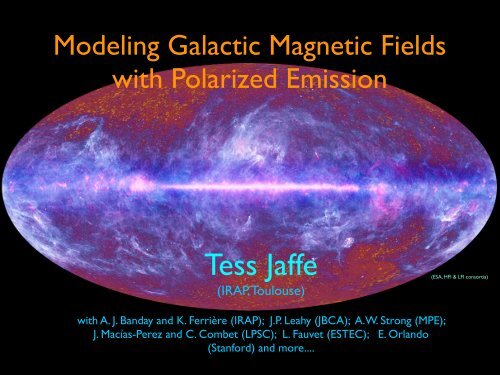
Modeling Galactic Magnetic Fieldswith Polarized EmissionTess Jaffe(IRAP, Toulouse)(ESA, HFI & LFI consortia)with A. J. Banday and K. Ferrière (IRAP); J.P. Leahy (JBCA); A.W. Strong (MPE);J. Macías-Perez and C. Combet (LPSC); L. Fauvet (ESTEC); E. Orlando(Stanford) and more....

Why are magnetic fields important?• They are everywhere. (The classical way to try to stump the colloquium speaker:“Have you considered the effect of ...?”)• They play key roles in:- primordial plasma physics;- galaxy formation and evolution;- hydrostatic balance in the ISM;- star formation via Parker instability;- turbulence (the other traditional way to try to stump the speaker) in both theISM and the IGM;- supernovae remnant expansion;- molecular cloud collapse;- ....• They are central to cosmic microwave background component separation.• They deflect ultra-high energy cosmic-rays (UHECRs).T. Jaffe @ ESAC, 30 May 2013

CMB foregrounds: Planck view(ESA, HFI & LFI consortia)•CMB observations in the sweet spotbetween different foregroundcomponents that would otherwisedominate.•At low frequencies (few 10s of GHz),the synchrotron dominates the CMB.•At high frequencies (few 100s ofGHz), the dust dominates.•Both are polarized.=> Magnetic fields.WMAP teamT. Jaffe @ ESAC, 30 May 2013

ffν/GHzFor the analysis of AME we assume a fixed electron temperatureof 8000External galaxies:K for T e for all regions, fitting only foroneEM. Noteexamplethat this is not the true EM but an effective EM over the 1 ◦ radiusaperture. We also allowed made fits allowing T e to vary, theresults of which are presented in Section 5.6.The thermal dust is fitted using a modified black body fit,S td = 2 h ν3c 2 1e hν/kT d − 1τ 250 (ν/1.2THz) β dΩ, (6)fitting for the optical depth τ 250 ,thedusttemperatureT d and theemissivity index β d .TheCMBisfittedusingthedifferential of ablack-body at T CMB = 2.726 K:( ) 2kΩν2S cmb =c 2 ∆T CMB . (7)where δT CMB is the CMB fluctuation temperature in thermodynamicunits. The spinning dust is fitted usingS sp = N H j ν Ω. (8)where we use a model for j ν calculated using the SPDUST (v2)code of Ali-Haïmoud et al. (2009); Silsbee et al. (2011). For themajority of sources we use fixed parameters appropriate to theWarm Ionized Medium (WIM) fitting only for the amplitude NHsdwhich has a peak frequency of ≈ 28 GHz. In a few sources, thepeak frequency appears to be at a lower frequency, in which casewe fit a Warm Neutral Medium (WNM) model, with a peak frequencyof ≈ 23 GHz.The least-squares fit was calculated using the MPFIT 8(Markwardt 2009) packagewritteninIDLwithstartingvaluesestimated from the data. We constrained amplitude parameters tobe positive and for the CMB fluctuation to be −150 < ∆T CMB

External galaxies: other examplesNGC6946 6cm PI over Hα (Copyright R. Beck, MPIfR)(Soida et al. 2002)A variety of morphologies observed, and we cannot assume a relationshipwith other matter tracers.T. Jaffe @ ESAC, 30 May 2013

Vertical fields in external Galaxies’• More often than not, thickdisk (“halo”) fields remainparallel to the plane. Butnot always, as seen here.• Again, we cannot see ourslike this or the fielddirection.• (Note: “thick disk” oftenreferred to as the ”halo”,extending of order a fewkpc off the plane.)Copyright Cracow ObservatoryT. Jaffe @ ESAC, 30 May 2013

Small-scale field: TurbulenceEMLS I and PI (Uyaniker et al. 1999)Magnetic energy spectrum from pulsar data (Han et al.2004)T. Jaffe @ ESAC, 30 May 2013

Observables• Synchrotron emission:i.e. traces component perpendicular to LOS• Rotation measure:i.e. traces component parallel to LOS and issensitive to the direction• Thermal dust emission: ? i.e. traces component perpendicular to LOSbut depends on dust environment, grain sizes and shapes, alignment mechanisms....• Starlight polarization, Zeeman splitting, masers, etc.• But: electron distributions not well known, dust polarized emission process not well known, datacontaminated with other stuff (bremsstrahlung, CMB, intrinsic RM, etc.)(Courtesy J.F. Macías-Pérez)T. Jaffe @ ESAC, 30 May 2013(Courtesy R. Wielebinski)

GeometryCoherent• Coherent contributes to RM for B|| and to Iand PI for Bperp.• Ordered random (i.e., the anisotropy in theturbulence) contributes to I and PIperpendicular, but to RM variance only.• Isotropic random contributes only to I and toPI and RM variance.RM > 0σRM = 0I = 0PI = 0RM = 0σRM = 0I > 0PI > 0Ordered randomRM = 0σRM = 0I > 0PI > 0Isotropic random•(At high frequencies, outside of Faradayregime.)• Careful when discussing “regular”, “random”,“turbulent”, etc.RM = 0σRM > 0I = 0PI = 0•Want I and PI at the same wavelength, butcannot on the plane.•Of previous results, only Jansson&Farrar takethis component into account.RM = 0σRM > 0I > 0PI = 0σPI > 0T. Jaffe @ ESAC, 30 May 2013

Radio Observations408 MHz total intensity (Haslam et al. 1982) 23 GH polarized intensity (Page et al. 2007)Faraday rotation measure (RM) 1.4 GHz(Taylor et al. 2010) Not shown: SGPS,CGPS, VLA data along the plane.T. Jaffe @ ESAC, 30 May 20131.4 GHz polarized intensity(Wolleben et al. 2006, Testori et al. 2008)

A very brief review of recent workT. Jaffe @ ESAC, 30 May 2013

RM-based modeling• With RMs, can study direction of field (from RM mean) andamount of turbulence along LOS (from RM variance).• Pulsar distance estimates probe along LOS, while extragalacticsources give better sampling and probe full disk.• But uncertainties in thermal electron distribution as well asrelated pulsar distance determinations.• The only certainty is that there are puzzling reversals.(Vallée et al. 2005)van Eck et al. (2011)T. Jaffe @ ESAC, 30 May 2013(Han et al. 2006)

Field reversals?• Reversals => dynamos or primordial?Example of numerical simulation of fieldgenerated by CR-driven dynamo in barredspiral (Kulpa-Dybełl et al. 2011)• Need a more detailed understanding ofwhere the fields are reversed, i.e. moreGalactic pulsar RMs.Examples of formation of bisymmetric spiral (BSS, left) or ring reversal(right) from primordial field (Sofue et al. 2010)T. Jaffe @ ESAC, 30 May 2013

RM + synchrotron models• Complementary observables to constrainboth LOS and plane-of-sky fieldcomponents.• Sun et al. (2008): RMs and synchrotron,include 1.4 GHz depolarization and EM analysis,both in the plane and off. But idealized CREsand B-field components. Unknown effect oflocal structures.(Sun et al. (2008)(courtesy X Sun. & W. Reich)• Jansson et al. (2009,2012): 23 GHz andRMs, MCMC analysis, vertical structure,“striated” (=”ordered random”) componentincluded (2012). But excludes plane, notprobing full disk. Unknown effect of localstructures.• Only Jansson et al. take into account theanisotropic turbulence, i.e. the “orderedrandom” field.T. Jaffe @ ESAC, 30 May 2013Jansson & Farrar (2012)

Local structure?• Sky visibly dominated by spurs and loops. How reliable are fits of large-scalefield models to synchrotron polarization?North polar spur (NPS)aka “Loop I”Synchrotron map at 408 MHz (Haslam et al. 1982).Figure from Page et al. (2007)T. Jaffe @ ESAC, 30 May 2013

First look at the plane• Step features in I: arm tangents?• Peaks and troughs in RM: arms?• Reversals?T. Jaffe @ ESAC, 30 May 2013

Modeling: hammurabi• Hammurabi Code* (Waelkens, Jaffe, et al. 2009)• HEALPix scheme for LOS integration of:• Faraday RM;• synchrotron I, Q, and U (with Faradayrotation applied);• thermal dust I, Q, U (ditto);• (EM);• (DM)...• Modular C++; add your own models.1.4 GHz polarized intensity* Publicly available on Sourceforge:http://sourceforge.net/projects/hammurabicode/23 GHz polarized intensity(Courtesy A. Waelkens.)T. Jaffe @ ESAC, 30 May 2013

Model inputs:Motivated by external galaxies:- 3D magnetic field model:• spiral arm model for ‘coherent’ field;• small-scale turbulence based on GRF with powerlawspectrum;• compression model amplifies and stretches intoanisotropic (‘ordered’) component along armridges based loosely on Broadbent (1989).- 3D CRE density and spectral model- 3D thermal electron density model, e.g., NE2001(Cordes and Lazio 2002);- Hammurabi to integrate observables along LOS;- MCMC (cosmoMC) engine to explore parameterspace.=> Powerful tool to- study the magnetized ISM using information from radioto γ-ray, and- to simulate polarized foregrounds with realisticturbulence for testing component separation forcosmology (for PRISM or Pixie).T. Jaffe @ ESAC, 30 May 2013

Cartoon example:T. Jaffe @ ESAC, 30 May 2013

Cartoon example:coherent• With a reasonable estimate for ne,RMs give Bcoh.T. Jaffe @ ESAC, 30 May 2013

Cartoon example:coherent+ isotropic random• With a reasonable estimate for ne,RMs give Bcoh.• Added simple homogeneous,isotropic GRF produces most of thetotal I but not its morphology.T. Jaffe @ ESAC, 30 May 2013

Cartoon example:coherent+ isotropic random+ inhomogeneous• With a reasonable estimate for ne,RMs give Bcoh.• Added simple homogeneous,isotropic GRF produces most of thetotal I but not its morphology.• Amplification of random field inarms (inhomogeneous), but stillisotropic, can fit total I but not PI.T. Jaffe @ ESAC, 30 May 2013

Cartoon example:coherent+ isotropic random+ inhomogeneous+ anisotropic• With a reasonable estimate for ne,RMs give Bcoh.• Added simple homogeneous,isotropic GRF produces most of thetotal I but not its morphology.• Amplification of random field inarms (inhomogeneous), but stillisotropic, can fit total I but not PI.• Random field stretched along arm giving“ordered random “ component in additionto the isotropic random component.T. Jaffe @ ESAC, 30 May 2013

Cartoon example:coherent+ isotropic random+ inhomogeneous+ anisotropic• With a reasonable estimate for ne,RMs give Bcoh.• Added simple homogeneous,isotropic GRF produces most of thetotal I but not its morphology.• Amplification of random field inarms (inhomogeneous), but stillisotropic, can fit total I but not PI.• Random field stretched along arm giving“ordered random “ component in additionto the isotropic random component.=> With three observables,constrain three field components:Bcoh, Biso, and BordT. Jaffe @ ESAC, 30 May 2013

First results:• 8 parameters fit: φ0, a0 - a4(arms+ring), BRMS, ford.• Orientation of spiral matches NE2001ne model.• Reversal in Scutum-Crux arm and“molecular ring”.• Coherent, isotropic random, orderedfield energy densities in ratios of 1:5:3(roughly 2, 4, and 3 μG along armridges, but this is model dependent).• Weak Sag-Carina arm? Mentioned inBenjamin et al. (2005) using GLIMPSEcounts. Two dominant arms?Reversals?Jaffe et al. (2010)Main limitation: assumes simple power-law CRE spectrum from 0.1 to 1000 GeV. ButCRE spectrum is degenerate with ford. To break the degeneracy, need an additionalfrequency.Interestingly, 2.3 GHz total I is not compatible with this model!T. Jaffe @ ESAC, 30 May 2013

CREs: or, real life isn’t always a power law.• Next step: link in GALPROP code of Strong and Moskalenko (2001)! Selfconsistentin the sense that GALPROP is given the same magnetic field fromhammurabi.• Use full integration over CRE energy spectrum at each point in the 3D galaxymodel:(see e.g. Rybicki & Lightman)• Add a synchrotron data point: 2.3 GHz total I from Jonas et al. (1998).• Add CRE model constrained by gamma-ray data (inverse Compton from thesame electrons); see Strong et al. (2010).T. Jaffe @ ESAC, 30 May 2013

CRE results:0.408 GHz(total I)2.3 GHz(total I)solar modulation23 GHz(PI)previously assumedJaffe et al. (2011)(See also Strong, Orlando, & Jaffe 2011)• Find below few GeV, J(E)∼E -1.3 ,slightly harder than usuallyassumed, compared to J(E)∼E -2.3above.• Note that at lower energies, solarmodulation affects localmeasurements.• Consistent with Strong, Orlando,& Jaffe (2011) high-latitude studyfrom 40 MHz to 23 GHz.• Two results: firstly, betterconstraint on B-fieldcomponents. Secondly,constraint on low-energy endof CRE spectrum otherwiseinaccessible.T. Jaffe @ ESAC, 30 May 2013

Dust: ongoing worksynch total Isynch PIsynch PI/Idust total Idust PIdust PI/IRM• Simple model for thermal dust polarization doesnot work even with sub-grid PI/I of 30%. Howinteresting!• Note also problem with VLA data. No simplespirals!• Polarization degree significantly under-predicted=> dust emission coming from regions with moreordered fields.• This means we can begin to separate arm ridges indifferent components.• Cannot do it by changing dust distribution alone.• This could be telling us about the detaileddistribution of the magnetic fields even from ourposition within the disk.• WMAP just sensitive enough to get a first look butnot more than a qualitative analysis. Needs Planck!Jaffe et al. (2013.)T. Jaffe @ ESAC, 30 May 2013

Spiral arm ridges: separable?Spiral arm shock triggering star formation? CO and microwave-band dust trace relativelycold molecular clouds, whose collapse is triggered in the shock. Downstream, star formationheats PAHs and dust that emit in sub-mm (ISO). So CO at shock front, star formationtrailing? What does this mean for the magnetic field components?M51 component ridges, Patrikeev et al. (2011)T. Jaffe @ ESAC, 30 May 2013

Spiral arm ridges: separable?synch total Isynch PIsynch PI/Idust total Idust PIdust PI/IRMJaffe et al. (2013)T. Jaffe @ ESAC, 30 May 2013

Arm modulation?• Model of shock compression in spiral arms predicts roughly a factor of four ratiobetween pre- and post-shock for the component of the fields parallel to the shock,for the gas and dust, and at least that for the CREs.• This is not observed in synchrotron in external galaxies (e.g. M51) but it’s not clearwhether the observations have the resolution given that the shock region could befairly narrow.• CRE sources are also not uniformly distributed, and the CREs may remain highlyinhomogeneous if the diffusion is highly anisotropic. Two effects, one in shock and onedownstream, effectively smoothing it out?M51 and field by Fletcher et al. (2011)T. Jaffe @ ESAC, 30 May 2013Effenberger et al. (2012)

Planck:Planck and IRAS composite image (ESA).• Planck project on large scale magnetic fieldmodeling using polarized dust mapped withunprecedented precision.• Using magnetic field geometry constrained byRM and synchrotron, we can study the dustdistribution in the disk of the Galaxy.• Polarized dust emission is then acomplementary observable independent ofCRE or thermal electron distributionuncertainties affecting synchrotron.• Can we probe polarized emissivity, e.g. as afunction of dust temperature, radiative torquemechanisms, etc.?• Informed by modeling of grain alignmentprocesses from detailed studies of smallregions, and perhaps vice versa.T. Jaffe @ ESAC, 30 May 2013

Small scales: turbulence and depolarization• depth depolarization, superposition of emission from a changing magnetic fielddirection along the line of sight; •Faraday depth depolarization, where at low frequencies, emission rotated as itpropagates (a.k.a. differential Faraday rotation);• beam depolarization, polarization orientation changes within the observingbeam.•=> Can model “Faraday screen”, polarization “canals”, and polarization“horizon”.T. Jaffe @ ESAC, 30 May 2013

Magnetic field modeling plansToo long “To Do” list:NPS★ the “Fan” region vs the depolarization band?=> scale height, outer turbulence scale, galaxy dynamics,MHD...Fan★ the North Polar Spur (NPS)?=> other spurs, microwave “haze”, or Fermi bubbles (seee.g. Caretti et al. 2013)?• high-latitude sky global or local? can we predict CR deflections?• starlight polarization and dust extinction from Gaia?• supernova remnant polarization morphologies?=> independent probe of ambient field geometry• the halo field, vertical structure, and CRE distribution?• Galactic bar?• which theoretical models of field amplification (e.g. CR-drivendynamo, etc.) are consistent with the observed morphology?• ...• C-BASS, S-PASS, GALFACTS, LOFAR, ASKAP,SKA, Gaia!FanNPSDepolarization bandTop: WMAP 23 GHz polarized intensity.Bottom: 1.4GHz polarized intensity (Reich & Testori)T. Jaffe @ ESAC, 30 May 2013

Radio spurs, microwave haze, and Fermi bubbles?Radio spurs: nearby SNRs? Or galacticcenter outflows? Understanding the“depolarization horizon” will help toplace lower limits on the distance tothe polarized emission.S-PASS view by Carretti et al. (2013)Top: 1.4GHz, bottom 23GHzT. Jaffe @ ESAC, 30 May 2013

Υ-ray gradient problem?• CREs that produce synchrotron alsoproduce Υ-rays through InverseCompton and gas collisions.Observed angular distributiondepends on:- Cosmic ray source distribution?Assumed supernovae, followingpulsars.- Anisotropic diffusion? Degenerate.- Vertical distribution scale height?Difficult to measure, 1

Prospects:• C-Band All Sky Survey (C-BASS) full sky, full Stokes, at 5 GHz. Important for CMB componentseparation, synchrotron and magnetic field modeling, etc.• GALFACTS polarization survey at 1.4GHz from Arecibo. An order of magnitude more extragalactic RMsources as well as diffuse polarized emission for RM synthesis. Can use hammurabi to model turbulence,depolarization horizon, SNa remnants, RM synthesis testing, ....• LOFAR to model fields in Galactic halo, particularly where fields weak, ionized gas tenuous.• PILOT, PIXIE, PRISM (?) for post-Planck sub-millimeter polarization• SKA...GALFACTS field (George et al., ADASS, 2010)T. Jaffe @ ESAC, 30 May 2013SKA simulation (Cordes)

External galaxies:• Most of the same questions apply.• A variety of morphologies are apparent inpolarized emission, with magnetic arms often,but often not, following arms seen in gas tracers.• Will use modified hammurabi to model whatwe will see with LOFAR and SKA (and maybeALMA for dust?).• Easier than our own Galaxy because we canlook from outside.• Harder because of a lack of RM measurements.But...M51 in optical (HST) with radio (5 GHz, VLA & Effelsberg)intensity contours and field directionsT. Jaffe @ ESAC, 30 May 2013

SKA!SKA will allow Faraday RM measurements of background sources to getnot only orientation but direction: reversals?Shamelessly stolen figure, simulation from B. Gaensler of M31with ~10000 background RM sources expected with SKA!T. Jaffe @ ESAC, 30 May 2013

Conclusions:(wake up!)• It’s a very exciting time to be studying galactic magnetic fields.• You need many different and complementary observables to study thegalactic magnetic field.• The days of conflicting models being consistent with the data due todegeneracies and uncertain inputs are numbered.• In the process of attempting to model the magnetic fields, we learnabout things from CRE spectra to dust distribution, shock compressionprocesses, and grain alignment.• The fact that our models don't fit very well is a Good Thing. It meansthere's a lot of information there and a lot to do.T. Jaffe @ ESAC, 30 May 2013