Reports - California Cooperative Oceanic Fisheries Investigations
Reports - California Cooperative Oceanic Fisheries Investigations
Reports - California Cooperative Oceanic Fisheries Investigations

You also want an ePaper? Increase the reach of your titles
YUMPU automatically turns print PDFs into web optimized ePapers that Google loves.
VOLUME 46 DECEMBER 2006
CALIFORNIA<br />
COOPERATIVE<br />
OCEANIC<br />
FISHERIES<br />
INVESTIGATIONS<br />
<strong>Reports</strong><br />
VOLUME 47<br />
January 1 to December 31, 2006<br />
Cooperating Agencies:<br />
CALIFORNIA DEPARTMENT OF FISH AND GAME<br />
UNIVERSITY OF CALIFORNIA, SCRIPPS INSTITUTION OF OCEANOGRAPHY<br />
NATIONAL OCEANIC AND ATMOSPHERIC ADMINISTRATION, NATIONAL MARINE FISHERIES SERVICE
CALCOFI COORDINATOR Elizabeth Venrick<br />
EDITOR Sarah M. Shoffler<br />
This report is not copyrighted, except where otherwise indicated, and may<br />
be reproduced in other publications provided credit is given to <strong>California</strong><br />
<strong>Cooperative</strong> <strong>Oceanic</strong> <strong>Fisheries</strong> <strong>Investigations</strong> and to the author(s). Inquiries<br />
concerning this report should be addressed to CalCOFI Coordinator, Scripps<br />
Institution of Oceanography, La Jolla, CA 92038-0218.<br />
Printed and distributed December 2006, La Jolla, <strong>California</strong><br />
ISSN 0575-3317<br />
EDITORIAL BOARD<br />
Elizabeth Venrick<br />
Roger Hewitt<br />
Laura Rogers-Bennett
CalCOFI Rep., Vol. 47, 2006<br />
CONTENTS<br />
In Memoriam<br />
Laurence E. Eber . . . . . . . . . . . . . . . . . . . . . . . . . . . . . . . . . . . . . . . . . . . . . . . . . . . . . . . . . . . . . . . . . . . . . .5<br />
I. <strong>Reports</strong>, Review, and Publications<br />
Report of the CalCOFI Committee . . . . . . . . . . . . . . . . . . . . . . . . . . . . . . . . . . . . . . . . . . . . . . . . . . . . . . 7<br />
Review of Some <strong>California</strong> <strong>Fisheries</strong> for 2005: Coastal Pelagic Finfish, Market Squid,<br />
Dungeness Crab, Sea Urchin, Abalone, Kellet’s Whelk, Groundfish, Highly Migratory<br />
Species, Ocean Salmon, Nearshor Live-Fish, Pacific Herring, and White Seabass . . . . . . . . . . . . . . . . . . 9<br />
The State of the <strong>California</strong> Current, 2005-2006: Warm in the North, Cool in the South<br />
William T. Peterson, Robert Emmett, Ralf Goericke, Elizabeth Venrick, Arnold Mantyla,<br />
Steven J. Bograd, Franklin B. Schwing, Roger Hewitt, Nancy Lo, William Watson, Jay Barlow,<br />
Mark Lowry, Steve Ralston, Karin A. Forney, Bertha E. Lavaniegos, William J. Sydeman,<br />
David Hyrenbach, Russel W. Bradley, Pete Warzybok, Francisco Chavez, Karen Hunter,<br />
Scott Benson, Michael Weise, and James Harvey . . . . . . . . . . . . . . . . . . . . . . . . . . . . . . . . . . . . . . . . . . . . 30<br />
Publications . . . . . . . . . . . . . . . . . . . . . . . . . . . . . . . . . . . . . . . . . . . . . . . . . . . . . . . . . . . . . . . . . . . . . . . 75<br />
II. Symposium of the CalCOFI Conference, 2005<br />
Symposium Introduction: CalCOFI: The Sum of the Parts . . . . . . . . . . . . . . . . . . . . . . . . . . . . . . . . . . . . .77<br />
Marine Mammal Monitoring and Habitat <strong>Investigations</strong> During CalCOFI Surveys<br />
M. S. Soldevilla, S. M. Wiggins, J. Calambokidis, A. Douglas, E. M. Oleson,<br />
and J. A. Hildebrand . . . . . . . . . . . . . . . . . . . . . . . . . . . . . . . . . . . . . . . . . . . . . . . . . . . . . . . . . . . . . . .79<br />
Secular Warming in the <strong>California</strong> Current and North Pacific. David Field, Dan Cayan,<br />
and Francisco Chavez . . . . . . . . . . . . . . . . . . . . . . . . . . . . . . . . . . . . . . . . . . . . . . . . . . . . . . . . . . . . . .92<br />
III. Scientific Contributions<br />
Shift in Size-at-age of the Strait of Georgia Population of Pacific Hake (Merluccius productus).<br />
Jacquelynne R. King and Gordon A. McFarlane . . . . . . . . . . . . . . . . . . . . . . . . . . . . . . . . . . . . . . . . . . .111<br />
Gimme Shelter: The Importance of Crevices to Some Fish Species Inhabiting a<br />
Deeper-Water Rocky Outcrop in Southern <strong>California</strong>.<br />
Milton S. Love, Donna M. Schroeder, Bill Lenarz, Guy R. Cochrane . . . . . . . . . . . . . . . . . . . . . . . . . . . .119<br />
Interannual and Spatial Variation in the Distribution of Young-of-the-year Rockfish<br />
(Sebastes spp.): expanding and coordinating a survey sampling frame.<br />
Keith M. Sakuma,Stephen Ralston, and Vidar G. Wespestad . . . . . . . . . . . . . . . . . . . . . . . . . . . . . . . . . .127<br />
Rockfish Resources of the South Central <strong>California</strong> Coast:<br />
Analysis of the Resource from Partyboat Data, 1980–2005.<br />
John Stephens, Dean Wendt, Debra Wilson-Vandenberg, Jay Carroll, Royden Nakamura,<br />
Erin Nakada, Steven Rienecke, and Jono Wilson . . . . . . . . . . . . . . . . . . . . . . . . . . . . . . . . . . . . . . . . . . .140<br />
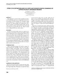
Temporal Patterns of the Siliceous Flux in the Santa Barbara Basin:<br />
The Influence of North Pacific and Local Oceanographic Processes.<br />
Elizabeth L. Venrick, Freda M. H. Reid, Amy Weinheimer, Carina B. Lange, E. P. Dever . . . . . . . . . . . . . .156<br />
Instructions to Authors . . . . . . . . . . . . . . . . . . . . . . . . . . . . . . . . . . . . . . . . . . . . . . . . . . . . . . . . . . . . . . . . . . 175<br />
CalCOFI Basic Station Plan . . . . . . . . . . . . . . . . . . . . . . . . . . . . . . . . . . . . . . . . . . . . . . . . . . . . . . inside back cover<br />
Indexed in Current Contents. Abstracted in Aquatic Sciences and <strong>Fisheries</strong> Abstracts and <strong>Oceanic</strong> Abstracts.
IN MEMORIAM<br />
CalCOFI Rep., Vol. 47, 2006<br />
Mathematician, meteorologist,<br />
computer scientist, Larry<br />
Eber’s career was propelled<br />
by tragedy and sustained by<br />
opportunities. The tragedy was<br />
the collapse of the Pacific sardine<br />
that propagated down<br />
the West Coast from Alaska<br />
to Baja <strong>California</strong>, Mexico in<br />
the mid 1940s. The Bureau of<br />
Commercial <strong>Fisheries</strong>’ Ocean Research Laboratory on<br />
the Stanford University campus was energized by the<br />
sardine collapse. Dr. Oscar Elton Sette established a longrange<br />
program to study the interaction of fisheries,<br />
oceanic and atmospheric physics, and biology of the<br />
North Pacific at Stanford University. For this purpose,<br />
Sette recruited an oceanographer, Ted Saur, and a meteorologist,<br />
Larry Eber. They began the Herculean task<br />
of extracting geostrophic wind estimates by entering<br />
and coding point pair differences in atmospheric pressure<br />
for wind-driven areas from the Oyashio exit from<br />
the Bering Sea across the North Pacific Current, the<br />
<strong>California</strong> Current, and its extension into the North<br />
Equatorial Current seasonally for 30 years. In addition<br />
to the quarterly time series of currents, they established<br />
a monthly mean time series of surface temperatures from<br />
two million ships’ log entries of engine intake temperatures<br />
from 1949–62).<br />
There were two main occurrences in Eber’s career.<br />
One was the invention and construction of electronic<br />
digital computers just before the middle of the 20th<br />
Century. Another was the great El Niño of 1957–58.<br />
The former gave Eber the tools for assembly, analyses,<br />
and display of summaries of great masses of meteorological<br />
and oceanographic data. His computer skills,<br />
learned at the UCLA Department of Meteorology, were<br />
honed at the Stanford Computation Center and the Fleet<br />
Numerical Weather Facility of the U.S. Navy, before the<br />
arrival of high-level computer languages like FORTRAN<br />
and BASIC. This gave him a decade of opportunity in<br />
bending the electronic digital computer to the tasks<br />
adopted by Sette, Saur and Eber. The great El Niño of<br />
1957–58 provided the climatic contrast necessary for<br />
IN MEMORIAM<br />
LAURENCE E. “LARRY” EBER<br />
1922–2005<br />
founding the science of interactions and climatic influences<br />
on the fisheries and biota.<br />
Following the founding of NOAA, the retirement of<br />
Dr. Sette, and closure of the Ocean Research Laboratory,<br />
Eber undertook the next phase of his career at NOAA’s<br />
Fishery Oceanography Center on the Scripps Institution<br />
of Oceanography Campus in the <strong>California</strong> <strong>Cooperative</strong><br />
<strong>Oceanic</strong> <strong>Fisheries</strong> <strong>Investigations</strong> (CalCOFI). On his arrival<br />
in 1970, there were only fledgling attempts at creating<br />
meteorological, oceanographic and biological<br />
databases from the preceding decades of data collection<br />
in the <strong>California</strong> Current habitat of the Pacific sardine.<br />
He derived and documented the procedure for locating<br />
weather satellite suborbital positions in 1973. In the<br />
5
IN MEMORIAM<br />
CalCOFI Rep., Vol. 47, 2006<br />
<strong>Fisheries</strong> Research Division he excelled in three functions:<br />
providing clean files of oceanographic data to other<br />
researchers; setting the mathematical procedures for establishing<br />
Julian day equations still used on CalCOFI<br />
cruises for estimation of contemporary physical oceanographic<br />
anomalies; and participating with Ron Lynn and<br />
Ken Bliss in the analysis of temperature, salinity, oxygen,<br />
stability, and geostrophic flow in the complex<br />
oceanic habitat of the <strong>California</strong> Current and adjacent<br />
regions. In the latter instance, Larry wrote the analysis<br />
software used on the CalCOFI data, as well as the<br />
EDMAP contouring programs for producing surface<br />
plots—programs that continued to be used by oceanography<br />
students and a wide array of his colleagues for<br />
decades after their inception. He subsequently joined<br />
biologists Geoff Moser and Paul Smith in describing the<br />
effect of the great 1957–58 El Niño on the habitat<br />
boundaries, biota, and physical properties of the<br />
<strong>California</strong> Current. He also joined Mark Ohman and<br />
6<br />
Paul Smith in the analysis of zooplankton spatial patterns<br />
using the Acoustic Doppler Current Profiler echo<br />
amplitude files.<br />
Larry Eber graduated from high school at Avalon,<br />
Catalina Island at the onset of World War II and attended<br />
Junior College and the UCLA Department of Meteorology<br />
where Jacob Bjerknes was his mentor. Eber’s war<br />
duty was with the First Cavalry Division in Australia,<br />
the Philippines, and Japan where he attained the rank<br />
of Staff Sergeant. He joined a team in Hawaii in a fruitless<br />
effort to induce more rainfall over pineapple plantations.<br />
In 1992, after 39 years of Federal service, he<br />
retired from NOAA Southwest <strong>Fisheries</strong> Science Center,<br />
La Jolla. Larry is survived by his wife of 56 years, Audrey,<br />
two children and two grandchildren.<br />
Eber’s modesty, creativity and service are sorely missed.<br />
Ron Dotson<br />
Paul Smith
COMMITTEE REPORT<br />
CalCOFI Rep., Vol. 47, 2006<br />
Part I<br />
REPORTS, REVIEW, AND PUBLICATIONS<br />
In 2005, participants in the CalCOFI Conference<br />
were offered the opportunity to register electronically.<br />
Those paying fees individually were encouraged to pay<br />
via PayPal using either a credit card or established PayPal<br />
account. This provides several advantages to the conveners<br />
(for instance, we no longer have to decode handwritten<br />
registration information, or handle large numbers<br />
of personal checks and cash). We have established a listserve<br />
for electronic communications. We have encouraged<br />
electronic registration for the 2006 conference and<br />
expect to continue this in the future. Because this is an<br />
evolving process, we welcome your feedback.<br />
At this writing, all published CalCOFI Atlases are<br />
being scanned and will be made available as searchable<br />
.pdf files on the Scripps/CalCOFI web site (www.<br />
calcofi.org; follow link to publications, then to atlases),<br />
much as the CalCOFI <strong>Reports</strong> have been. Ultimately,<br />
we hope to link the Atlases with the underlying data.<br />
PACOOS<br />
The <strong>California</strong> Current flows affect the ecology,<br />
weather, climate and economies of the entire West Coast<br />
of North America. The Pacific Coast Ocean Observing<br />
System (PaCOOS) is an umbrella organization of federal<br />
and state agencies and academic partners that is developing<br />
ocean-observing products and services that are<br />
transboundary in nature and apply to the entire region<br />
(three countries and three Regional Associations). The<br />
present focus is on data management and modeling activities<br />
leading eventually towards ecological forecasts.<br />
There is an annual Board of Governors meeting and ad<br />
hoc Committees on data management, modeling, and<br />
ocean observing. More information about PaCOOS can<br />
be found at (www.pacoos.org). Under the auspices of<br />
PaCOOS, the following activities relating to CalCOFI<br />
occurred in the 2005–06 timeframe:<br />
1. Reoccupation of the CalCOFI survey line off<br />
Humbolt, CA conducted by NOAA and Humbolt<br />
State University began in May 2006.<br />
2. Monterey Bay Area Research Institute (MBARI), the<br />
Naval Post-Graduate School and the University of<br />
<strong>California</strong>, Santa Cruz (UCSC) continue to conduct<br />
the quarterly central-<strong>California</strong> CalCOFI survey line.<br />
REPORT OF THE CALCOFI COMMITTEE<br />
3. A quarterly Oregon survey line off of Newport, OR<br />
by NOAA began in April 2006.<br />
4. NOAA and PaCOOS partners continue to develop<br />
data management capabilities; eventually the following<br />
ecological data will be served online:<br />
a. West Coast oceanographic data including the<br />
NOAA CalCOFI dataset (http://www.pfeg.noaa.<br />
gov/products/las.html),<br />
b. West Coast benthic habitat data that will be available<br />
online in 2006,<br />
c. National Marine Sanctuary West Coast data,<br />
d. Krill time-series data in southern and central<br />
<strong>California</strong> by Scripps Institution of Oceanography<br />
and University of <strong>California</strong>, Santa Cruz.<br />
The PaCOOS governing body also matured with the<br />
establishment of an Executive Committee and coordinators<br />
at both the NOAA Northwest and Southwest<br />
<strong>Fisheries</strong> Science Centers as well as two academics representing<br />
the interests of the Regional Associations. Two<br />
workshops occurred in 2006 on biological data management<br />
and integration of CalCOFI data with ecological<br />
and physical data from Mexican and Canadian<br />
counterparts as well as on biological survey sampling<br />
methodologies for the <strong>California</strong> Current.<br />
SCCOOS<br />
Since July 2004, funding from the Southern <strong>California</strong><br />
Coastal Observing System (SCCOOS) has allowed<br />
CalCOFI surveys to occupy a suite of nine stations near<br />
or on the 20 fm depth contour. Preliminary examination<br />
of the physical, chemical, and bulk biological parameters<br />
indicates that the nearshore high-production<br />
zone is well covered by SCCOOS stations and by some<br />
CalCOFI inshore stations. Ongoing work focuses on<br />
differences in community structure and differences in<br />
the abundance of fish larvae in the nearshore and the<br />
CalCOFI coastal stations.<br />
CCE/LTER<br />
In 2004, the CalCOFI region was recognized by the<br />
National Science Foundation as a Long-Term Ecological<br />
Research area: the <strong>California</strong> Current Ecosystem (CCE).<br />
In May, the program initiated its first experimental process<br />
7
COMMITTEE REPORT<br />
CalCOFI Rep., Vol. 47, 2006<br />
cruise in the <strong>California</strong> Current System. The objective<br />
was to utilize the spatial variability in nitracline depth<br />
and food-web structure as an analog of the ecosystem<br />
change that has been observed over time by the<br />
CalCOFI surveys. Accordingly, the process cruise was<br />
structured around five experimental cycles, each in different<br />
hydrographic and biotic conditions including:<br />
active upwelling sites, the low-salinity core of the<br />
<strong>California</strong> Current, and the highly stratified offshore<br />
domain. The location of each cycle was determined<br />
with the help of the CalCOFI cruise 0604, MODIS<br />
satellite imagery, and Spray glider mapping. At each experimental<br />
cycle, a Globalstar satellite-tracked drifter<br />
array was deployed. This vertical array included a series<br />
of experimental incubation bottles for assessing grazing<br />
and growth rates of different constituents of the plankton<br />
assemblage. All sampling (for diel periodicity of<br />
mesozooplankton grazing, MOCNESS, iron-limitation<br />
incubations, dissolved organic matter, bio-optical properties,<br />
and other studies) were carried out in the<br />
Lagrangian context established by the drifter. Many of<br />
the cruise data will soon be accessible at the CCE web<br />
site (http://cce.lternet.edu/).<br />
GLIDER AND MVP HIGHLIGHTS<br />
Funds from the Gordon and Betty Moore foundation<br />
to M. Ohman and R. Davis at Scripps Institution<br />
of Oceanography purchased two autonomous Spray<br />
Gliders that are programmed to undulate continuously<br />
between 0 and 500 m, one proceeding along line 93 and<br />
one along line 80. The first glider was launched along<br />
line 93 in April 2005 and, as of this writing, has made<br />
three trips; the second was launched along line 80<br />
in October 2005 and has completed one trip. Selected<br />
profiles and data are available on the Spray web site<br />
(http://spray.ucsd.edu/; follow the link to Data).<br />
Also, Moore Foundation funds purchased a Moving<br />
Vessel Profiler (MVP) a free-fall instrument package<br />
equipped with a CTD, a fluorometer, and a Laser Optical<br />
Particle Counter that can be deployed and retrieved from<br />
a moving ship. This was successfully used for the first<br />
8<br />
time on CalCOFI 0511. Funds are being sought for routine<br />
deployment on CalCOFI cruises.<br />
HERRING MANDATE HIGHLIGHTS<br />
The <strong>California</strong> Fish and Game Commission adopted<br />
regulations to reduce the minimum mesh size from<br />
2-1/8 inches to 2 inches for the San Francisco Bay commercial<br />
herring gillnet fishery. The <strong>California</strong> Fish and<br />
Game Department expressed concern that a potential<br />
increase in the harvest of younger fish may have a longterm<br />
negative effect on the population. Since the<br />
1997–98 El Niño, larger, older fish have been scarce or<br />
absent in both catch and population samples, declining<br />
well below long-term averages. One of the principal<br />
management goals is to harvest age-4 fish and older from<br />
the population; this is designed to restore and maintain<br />
the herring fishery. The Department of Fish and Game<br />
provided an analysis of the potential impacts of reducing<br />
the mesh size in the Commission’s Supplement<br />
Environmental Document: Pacific Herring, Commercial<br />
Fishing Regulations. The Department determined that<br />
the use of 2-inch mesh would potentially increase the<br />
catch of 3- and possibly some 2-year-old fish. As mitigation<br />
for the potential take of the younger age-classes,<br />
the Department recommended reducing the quota at<br />
10 percent of spawning biomass (5,890 tons) by the<br />
percentage of 2- and 3-year-old herring estimated<br />
to comprise the 2004–05 season landings (11.3 and<br />
12.2 percent by weight respectively). The estimated percentage<br />
of 2- and 3-year-old herring is suggested as an<br />
approximation of the percentage that may be caught in<br />
the 2005–06 season. This results in a quota of 4,502 tons<br />
or 7.6 percent of the 2004–05 estimated spawning biomass.<br />
The Commission adopted the reduced quota for<br />
the 2005–06 season.<br />
The CalCOFI Committee:<br />
Elizabeth Venrick, UCSD<br />
Laura Rogers-Bennett, CDFG<br />
Roger Hewitt, NMFS
FISHERIES REVIEW<br />
CalCOFI Rep., Vol. 47, 2006<br />
REVIEW OF SOME CALIFORNIA FISHERIES FOR 2005:<br />
COASTAL PELAGIC FINFISH, MARKET SQUID, DUNGENESS CRAB, SEA URCHIN, ABALONE,<br />
KELLET’S WHELK, GROUNDFISH, HIGHLY MIGRATORY SPECIES, OCEAN SALMON,<br />
NEARSHORE LIVE-FISH, PACIFIC HERRING, AND WHITE SEABASS<br />
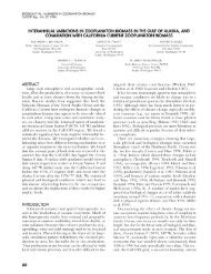
SUMMARY<br />
In 2005, commercial fisheries landed an estimated<br />
132,600 metric tons (t) of fishes and invertebrates from<br />
<strong>California</strong> ocean waters (fig. 1). This represents a decrease<br />
in landings of over 3% from the 137,329 t landed<br />
in 2004 and a 47% decline from the 252,568 t landed<br />
in 2000. In a shift from recent increasing trends, the preliminary<br />
ex-vessel economic value of commercial landings<br />
in 2005 was $107 million, a decrease of 19% from<br />
the $131 million in 2004, mainly the result of a sharp<br />
decline in Dungeness crab landings.<br />
After a one-year absence, market squid was once again<br />
the largest fishery in the state, both by volume at nearly<br />
56,000 t, and in ex-vessel value at $31.6 million. Pacific<br />
sardine slipped to second in landings at nearly 35,000 t,<br />
while the other top five <strong>California</strong> landings included<br />
northern anchovy at over 11,000 t, red sea urchin at<br />
over 5,000 t, and Dungeness crab at 4,500 t. The exvessel<br />
value of Dungeness crab ranked second at nearly<br />
$17 million. This is nearly a 60% decline from 2004<br />
($40.5 million). Other top five valued fisheries include<br />
Chinook salmon at nearly $13 million, red sea urchin<br />
at over $6 million, and <strong>California</strong> spiny lobster at nearly<br />
$6 million.<br />
Statewide landings of red sea urchin dropped nearly<br />
9% while exports for all sea urchin producing states declined<br />
by 21%. Fishing effort for red urchin has remained<br />
constant in southern <strong>California</strong>; however, effort<br />
in northern <strong>California</strong> has declined dramatically.<br />
Commercial landings of Pacific herring also continued<br />
to decline in 2005. An expanding fishery for Kellet’s<br />
whelk, usually taken as bycatch in lobster and crab traps<br />
in southern <strong>California</strong>, yielded 47 t, an increase of 33%<br />
over 2004 landings.<br />
<strong>California</strong>’s commercial groundfish harvest for 2005<br />
was over 10,000 t, a 16% decrease from 2004 landings.<br />
The groundfish harvest consisted mainly of Pacific whiting,<br />
Dover sole, sablefish, and rockfishes. Ex-vessel value<br />
of groundfish landings for 2005 was $13.8 million, similar<br />
to 2004. The Pacific <strong>Fisheries</strong> Management Council<br />
(PFMC) approved stock assessments for 18 groundfish<br />
species and removed lingcod from overfished status and<br />
considered the stock to be officially rebuilt.<br />
CALIFORNIA DEPARTMENT OF FISH AND GAME<br />
Marine Region<br />
8604 La Jolla Shores Drive<br />
La Jolla, CA 92037<br />
DSweetnam@dfg.ca.gov<br />
Figure 1. <strong>California</strong> ports and fishing areas.<br />
For highly migratory species (HMS), commercial and<br />
recreational landings of albacore decreased 35% and 53%,<br />
respectively, from 2004 landings. Bigeye tuna commercial<br />
landings decreased by 57% in the state. In addition,<br />
the PFMC declared that overfishing of bigeye tuna is occurring<br />
throughout its range in the eastern Pacific Ocean.<br />
In 2005, the <strong>California</strong> Fish and Game Commission<br />
(Commission) undertook 16 rule-making actions that<br />
address marine and anadromous species. The Commission<br />
also adopted the Abalone Recovery and Management<br />
Plan, which provides a cohesive framework for the recovery<br />
of depleted abalone populations in southern<br />
<strong>California</strong>, and for the management of the northern<br />
<strong>California</strong> fishery and future fisheries. All of <strong>California</strong>’s<br />
abalone species are included in this plan. In addition,<br />
9
FISHERIES REVIEW<br />
CalCOFI Rep., Vol. 47, 2006<br />
the Commission instituted a deep-water Tanner Crab<br />
fishery and created transferable lobster operator permits.<br />
Coastal Pelagic Finfish<br />
Pacific sardine (Sardinops sagax), Pacific mackerel<br />
(Scomber japonicus), jack mackerel (Trachurus symmetricus),<br />
and northern anchovy (Engraulis mordax) form a complex<br />
known as coastal pelagic species (CPS) finfish, all<br />
of which are jointly managed by the PFMC and NOAA<br />
<strong>Fisheries</strong>. In 2005, combined commercial landings of<br />
CPS finfish totaled 49,219 t (tab. 1), and the ex-vessel<br />
value exceeded $4.8 million (U.S.). The Pacific sardine<br />
fishery is the most valuable fishery among these four<br />
species, contributing 70% of the total tonnage and 65%<br />
of the total ex-vessel value.<br />
Pacific Sardine. The Pacific sardine fishery extends<br />
from British Columbia, Canada, southward into Baja<br />
<strong>California</strong>, México (BCM). Although historically the<br />
bulk of the catch has been landed in southern <strong>California</strong><br />
and Ensenada, BCM, landings in the Pacific Northwest<br />
have been increasing. In 2005, Oregon landings surpassed<br />
those of <strong>California</strong> for the first time since the sardine<br />
fishery expanded.<br />
The Pacific sardine harvest guideline (HG) for each<br />
calendar year is determined from the previous year’s<br />
stock biomass estimate (the number of age 1+ fish on<br />
1 July) in U.S. and Mexican waters. The 1 July 2004<br />
10<br />
TABLE 1<br />
Landings of Coastal Pelagic Species in <strong>California</strong> (metric tons)<br />
Year Pacific sardine Northern anchovy Pacific mackerel Jack mackerel Pacific herring Market squid Total<br />
1977 5 99,504 5,333 44,775 5,200 12,811 167,628<br />
1978 4 11,253 11,193 30,755 4,401 17,145 74,751<br />
1979 16 48,094 27,198 16,335 4,189 19,690 115,542<br />
1980 34 42,255 29,139 20,019 7,932 15,385 114,764<br />
1981 28 51,466 38,304 13,990 5,865 23,510 133,163<br />
1982 129 41,385 27,916 25,984 10,106 16,308 121,828<br />
1983 346 4,231 32,028 18,095 7,881 1,824 64,405<br />
1984 231 2,908 41,534 10,504 3,786 564 59,527<br />
1985 583 1,600 34,053 9,210 7,856 10,275 63,577<br />
1986 1,145 1,879 40,616 10,898 7,502 21,278 83,318<br />
1987 2,061 1,424 40,961 11,653 8,264 19,984 84,347<br />
1988 3,724 1,444 42,200 10,157 8,677 36,641 102,843<br />
1989 3,845 2,410 35,548 19,477 9,046 40,893 111,219<br />
1990 2,770 3,156 36,716 4,874 7,978 28,447 83,941<br />
1991 7,625 4,184 30,459 1,667 7,345 37,388 88,668<br />
1992 17,946 1,124 18,570 5,878 6,318 13,110 62,946<br />
1993 13,843 1,954 12,391 1,614 3,882 42,708 76,392<br />
1994 13,420 3,680 10,040 2,153 2,668 55,395 85,929<br />
1995 43,450 1,881 8,667 2,640 4,475 70,278 131,391<br />
1996 32,553 4,419 10,286 1,985 5,518 80,360 135,121<br />
1997 46,196 5,718 20,615 1,161 11,541 70,257 155,488<br />
1998 41,056 1,457 20,073 970 2,432 2,895 68,646<br />
1999 56,747 5,179 9,527 963 2,207 91,950 164,945<br />
2000 53,586 11,504 21,222 1,135 3,736 118,827 209,144<br />
2001 51,811 19,187 6,924 3,615 2,715 86,203 170,080<br />
2002 58,353 4,643 3,367 1,006 3,339 72,878 143,586<br />
2003 34,292 1,547 3,999 155 1,780 44,965 88,741<br />
2004 44,293 6,793 3,569 1,027 1,596 40,324 99,606<br />
2005 34,331 11,091 3,243 199 217 54,976 104,057<br />
stock biomass estimate for Pacific sardine was 1.2 million<br />
t and the recommended U.S. HG for the 2004<br />
season was 136,179 t. The southern sub-area (south of<br />
39˚N latitude to the U.S.-México Border) received twothirds<br />
of the HG (90,786 t) and the northern sub-area<br />
(north of 39˚N latitude to the U.S.-Canada Border)<br />
received one-third (45,393 t). On 1 September, 80%<br />
(68,106 t) of the uncaught HG was reallocated to the<br />
southern sub-area, and 20% (17,026 t) was reallocated<br />
to the northern sub-area. On 1 December, the total remaining<br />
HG (54,200 t) was opened coast-wide, and by<br />
31 December 2005, 63% (86,430 t) of the HG had been<br />
caught coast-wide.<br />
After considering a number of alternatives for a different<br />
allocation scheme for the U.S. West Coast, the<br />
PFMC decided on a seasonal coast-wide framework in<br />
June 2005, effective for the 2006 season. On 1 January,<br />
35 % of the total U.S. HG will be allocated coast-wide.<br />
On 1 July, 40% of the HG, plus the uncaught remainder<br />
of the previous allocation, will be allocated coastwide.<br />
Then, on 15 September, the remaining 25% of<br />
the HG, plus any unharvested remainder, will be allocated<br />
coast-wide. U.S. tribes have also shown interest<br />
in a portion of the sardine HG. Once a tribal allocation<br />
is decided, it will be applied to the coast-wide HG<br />
first; the non-tribal allocation will apply to the remainder,<br />
after the tribal allocation is accommodated.
FISHERIES REVIEW<br />
CalCOFI Rep., Vol. 47, 2006<br />
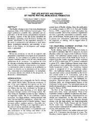
Figure 2. <strong>California</strong> commercial landings of Pacific sardine (Sardinops<br />
sagax) and Pacific mackerel (Scomber japonicus), 1984–2005.<br />
Because of uncertainties inherent in the fishery and sardine<br />
population, the new framework will be reevaluated<br />
in 2008.<br />
During 2005, 34,599 t of Pacific sardine, valued at<br />
more than $3.2 million, was landed in <strong>California</strong>. This<br />
represents a 21.9% decrease in commercial sardine landings<br />
from 2004 (44,293 t). In <strong>California</strong>, commercial<br />
sardine landings averaged 45,176 t over the ten-year<br />
period from 1995–2005 (fig. 2). As in previous years,<br />
most (93.4%) of <strong>California</strong>’s 2005 catch was landed in<br />
the Los Angeles (69.9%; 24,173.7 t) and Monterey<br />
(23.5%; 8,117.9 t) port areas (tab. 2).<br />
During 2005, a total of 31,800.5 t of sardine product<br />
was exported from <strong>California</strong> to 33 countries. Most of<br />
this product was exported to Australia (16,625.6 t), Japan<br />
(7,154.8 t), China (3,222.1 t), and South Korea (2,192.3 t),<br />
which represents more than 91% of the total export value<br />
of nearly $15.9 million.<br />
Oregon’s sardine landings have increased steadily over<br />
the past few years (fig. 3) and, for the first time, exceeded<br />
<strong>California</strong>’s landings in 2005. A total of 45,110 t of sardines<br />
with an ex-vessel value of nearly $6.2 million was<br />
landed in Oregon during 2005. This represents a 30%<br />
increase over 2003 (25,258 t). In contrast, Washington’s<br />
2004 sardine landings decreased by 25% to 8,934 t in<br />
2004, compared to 11,920 t in 2003 (fig. 3).<br />
Pacific Mackerel. Although Pacific mackerel is occasionally<br />
landed in Oregon and Washington, the majority<br />
of landings are made in southern <strong>California</strong> and<br />
Ensenada, BCM. The U.S. fishing season for Pacific<br />
mackerel runs from 1 July to 30 June. At the beginning<br />
of the 2005–06 season (1 July 2005), the biomass<br />
was estimated to be 81,383 t and the HG was set at<br />
17,419 t. Because mackerel are often landed incidentally<br />
to other CPS, the HG was divided into a directed fish-<br />
Figure 3. Commercial landings of Pacific sardine (Sardinops sagax) in<br />
<strong>California</strong>, Oregon, and Washington, 1999–2005 (PacFIN data).<br />
TABLE 2<br />
Landings of Pacific sardine (Sardinops sagax) and Pacific<br />
mackerel (Scomber japonicus) at <strong>California</strong> Port Areas<br />
Pacific Sardine Pacific Mackerel<br />
Area Landings t % Total t Landings t % Total t<br />
Eureka 0.0 0.0 0.0 0.00<br />
San Francisco 308.9 0.9 0.0 0.00<br />
Monterey 8,117.9 23.5 0.4 0.01<br />
Santa Barbara 1,976.9 5.7 97.0 2.99<br />
Los Angeles 24,173.7 69.9 3,144.9 96.97<br />
San Diego 21.5 0.1 1.0 0.03<br />
Total 34,598.9 100.0 3,243.3 100.0<br />
ery (13,419 t) with the remaining HG (4,000 t) set aside<br />
for incidental catch (limited to 40% of a mixed load).<br />
<strong>California</strong> landings of Pacific mackerel have been declining<br />
since the early 1990s (fig. 2). Over the last ten<br />
years, annual landings have averaged 10,136 t; however,<br />
since 2002, they have not exceeded 4,000 t. In 2005,<br />
3,243 t of Pacific mackerel were landed in <strong>California</strong><br />
with an ex-vessel value of $535,259. Ninety-seven percent<br />
(3,145 t) was landed in the Los Angeles port areas<br />
(tab. 2).<br />
<strong>California</strong> exported 1,311 t of mackerel product to<br />
thirteen countries worldwide. Most (56%) of this product<br />
was exported to Australia and Indonesia. Mackerel<br />
exporters generated $0.8 million in export revenue in<br />
2005. Since 1999, an average of 211 t of Pacific mackerel<br />
has been landed in Oregon, and 318 t was landed<br />
during 2005. In Washington, annual landings of mackerel<br />
(unspecified species) have averaged 144 t since the<br />
year 2001; however, only 24 t were landed in 2005.<br />
Jack Mackerel. Landings of jack mackerel in<br />
<strong>California</strong> dropped in 2005 (278 t) from the previous<br />
year (1,027 t); this is only about 100 tons more than the<br />
11
FISHERIES REVIEW<br />
CalCOFI Rep., Vol. 47, 2006<br />
most recent low of 141 t in 2003. Ex-vessel revenues in<br />
2005 totaled $50,833, a 79% decrease from 2004. In<br />
Oregon, landings of jack mackerel totaled 69.8 t with<br />
an ex-vessel value of $19,489. This represents a 41% decrease<br />
in landings from 2004 and a 93% increase from<br />
2003. There were no reported landings of jack mackerel<br />
in Washington during 2005.<br />
Northern Anchovy. Over the past decade, landings<br />
of northern anchovy in <strong>California</strong> have varied widely.<br />
Anchovy landings increased again in 2005, when they<br />
totaled 11,178 t, up 39% over the previous year (6,793 t).<br />
Ex-vessel revenues for northern anchovy totaled $1.1 million,<br />
making this species the second most valuable CPS<br />
finfish in 2005, behind Pacific sardine. In terms of total<br />
ex-vessel revenues realized by the four CPS finfish, Pacific<br />
sardine represented 65.4%, northern anchovy 22.4%,<br />
Pacific mackerel 11.1%, and jack mackerel 1.1%.<br />
<strong>California</strong> exported 160 t of anchovy product, valued<br />
at $534,231, to four countries in 2005, an increase<br />
of three times the weight and nearly two times the value<br />
of 2004. Sixty-eight percent of <strong>California</strong>’s anchovy export<br />
product was shipped to Australia (108 t; $355,656).<br />
In 2005, no northern anchovy was landed in Washington.<br />
Oregon, however, landed 68.4 t valued at $1,576.<br />
Krill. Krill are composed of several species of euphausiids,<br />
small shrimp-like crustaceans that serve as the<br />
basis of the food web for many commercially fished<br />
species, as well as marine mammals and birds. Krill fisheries<br />
exist in other parts of the world, where they are<br />
primarily used for bait and as feed for pets, cultured fish,<br />
and livestock. Following a request from the National<br />
Marine Sanctuaries to prohibit krill fishing in the exclusive<br />
economic zone (EEZ) around the three marine<br />
sanctuaries off central <strong>California</strong>, the PFMC initiated an<br />
amendment to the CPS FMP to include krill as a management<br />
unit. State laws already prohibit the landing of<br />
krill in all Washington, Oregon, and <strong>California</strong> ports.<br />
After evaluating alternatives presented in an environmental<br />
assessment, the PFMC adopted a wider ban on<br />
all commercial fishing for krill in federal U.S. waters,<br />
and also designated essential fish habitat (EFH) for krill<br />
in order to more easily work with other federal agencies<br />
to protect krill.<br />
<strong>California</strong> Market Squid<br />
In 2005, the market squid (Loligo opalescens) was the<br />
state’s largest fishery, both in quantity and ex-vessel value.<br />
Total landings in the squid fishery were 20% greater than<br />
in 2004, increasing from 46,323 t to 55,606 t (fig. 4).<br />
The ex-vessel price ranged from $330-$992/t, with an<br />
average of $569/t (an increase over the average of $450/t<br />
in 2004). The 2005 ex-vessel value was approximately<br />
$31.6 million, a 59% increase from 2004 ($19.9 million).<br />
Market squid is used domestically for food and bait and<br />
12<br />
remains an important international commodity. Approximately<br />
43,131 t of market squid were exported for a<br />
value of $54.6 million in 2005. Asian countries were the<br />
main export market with about 73% of the trade going<br />
to China and Japan.<br />
The fishery uses either seine or brail gear that is usually<br />
combined with attracting lights to capture shallowspawning<br />
squid populations in areas over sandy substrate.<br />
Spawning may occur year-round; however, the fishery<br />
is most active from April to September in central<br />
<strong>California</strong>, and from October to March in southern<br />
<strong>California</strong>. The fishing permit season for market squid<br />
extends from 1 April through 31 March of the following<br />
year. During the 2005–06 season (as opposed to the<br />
2005 calendar year), 70,972 t were landed, a 54% increase<br />
from the 2004–05 season (46,211 t). There was a<br />
69% decline in catch from the northern fishery near<br />
Monterey in the 2005–06 season with only 2,046 t landed<br />
(fig. 5). As in previous seasons, total catch was greater<br />
in southern <strong>California</strong>, with 68,925 t landed (97% of<br />
the catch) during the 2005–06 season (fig. 5). In 2005–06,<br />
squid fishing centered mainly around Catalina Island—<br />
whereas in the 2004–05 season, fishing activity took<br />
place primarily in areas around the northern Channel<br />
Islands near Santa Rosa and Santa Cruz Islands and along<br />
the Port Hueneme coast.<br />
To protect and manage the squid resource, a market<br />
squid fishery management plan (MSFMP) was adopted<br />
by the Commission in 2004. Goals of the MSFMP were<br />
developed to ensure sustainable long-term conservation<br />
and to provide a management framework that is responsive<br />
to environmental and socioeconomic changes.<br />
The 2005–06 fishing season marked the inaugural year<br />
that a restricted access program was implemented under<br />
the MSFMP. A total of 170 restricted access permits were<br />
issued: 77 transferable vessel permits, 14 non-transferable<br />
vessel permits, 14 transferable brail permits, 64 light<br />
boat permits, and 1 experimental non-transferable vessel<br />
permit.<br />
Because market squid live, on average, six to nine<br />
months, reproduce at the end of their lifespan, and<br />
are harvested on spawning grounds, it is critical that<br />
the management of the fishery allows for an adequate<br />
number of eggs to be spawned prior to harvest.<br />
Biological sampling, carried out by CDFG, is designed<br />
to monitor the proportion of the population allowed<br />
to spawn before being captured by the fishery. The<br />
“egg escapement method,” which estimates the level<br />
of reproductive output from fished stocks and is used<br />
as a proxy for maximum sustainable yield, is described<br />
in the 2002 Federal CPS FMP. By spring 2007, the<br />
PFMC Coastal Pelagic Species Management Team<br />
will review the egg escapement method and its management<br />
implications.
FISHERIES REVIEW<br />
CalCOFI Rep., Vol. 47, 2006<br />
Figure 4. <strong>California</strong> commercial market squid (Loligo opalescens) Landings, 1982–2005.<br />
Figure 5. Comparison of market squid (Loligo opalescens) landings for northern and southern fisheries by fishing season (1 April–31 March),<br />
from the 1982–83 season to 2005–06 season.<br />
13
FISHERIES REVIEW<br />
CalCOFI Rep., Vol. 47, 2006<br />
Figure 6. <strong>California</strong> commercial Dungeness crab (Cancer magister) landings,<br />
1981–2005.<br />
Dungeness Crab<br />
Landings of Dungeness crab (Cancer magister) in 2005<br />
were estimated at 4,501 t, a 60% decrease from the<br />
11,281 t landed in 2004, which were the highest landings<br />
in 25 years (fig. 6). This ends the trend of increased<br />
landings since 2001, which had the lowest landings in<br />
25 years. Ex-vessel revenues for 2005 were $16.6 million,<br />
a 59% decrease in value from 2004 ($40.5 million).<br />
The average price per kilogram increased 2% from $3.59<br />
in 2004 to $3.68 in 2005.<br />
Legislation to authorize a preseason soft-shell testing<br />
program was introduced during 1994, and industryfunded<br />
preseason testing began prior to the 1995–96<br />
season. The legislation mandates that at least 25% of the<br />
meat is picked out and is monitored by the Pacific States<br />
Marine <strong>Fisheries</strong> Commission. The program is initiated<br />
each year around 1 November; if the crab meat recovery<br />
is less than 25%, another test is mandated. Two weeks<br />
later the second test is conducted, and if the pick-out<br />
is still below 25%, the season opening is delayed 15 days.<br />
This procedure can continue until 1 January, when no<br />
more tests can be made and the season must be opened<br />
on 15 January. Tests conducted on 1 November and<br />
17 November yielded an average recovery of less than<br />
25%, which resulted in a postponement of the opening<br />
in Del Norte, Humboldt, and Mendocino counties until<br />
December 16. Subsequent tests conducted on 7 December<br />
yielded similar results, which led to a second 15-day<br />
postponement through 31 December 2005. In accordance<br />
with a tri-state management compact, Oregon<br />
and Washington delayed their season openings, so that<br />
the entire West Coast fishery north of Point Arena<br />
opened at the same time. The significant decrease in<br />
landings in 2005 from 2004 is directly attributable to<br />
this 30-day delay in the season opening in these three<br />
14<br />
counties, which contributed 75% of the annual statewide<br />
catch in 2004.<br />
The Dungeness crab fishery in <strong>California</strong> is managed<br />
under a regimen of size, sex, and season. Only male<br />
Dungeness crabs are harvested commercially, and the<br />
minimum commercial harvest size is 159 mm (6.25 in),<br />
measured by the shortest distance across the carapace<br />
immediately in front of the posterior lateral spines. The<br />
minimum size limit is designed to protect sexually mature<br />
crabs from harvest for one or two seasons, and the<br />
timing of the season is designed to provide some measure<br />
of protection to crabs when molting is most prevalent.<br />
<strong>California</strong> implemented regulations prohibiting the<br />
sale of female Dungeness crabs in 1897. Minimum size<br />
regulations were first implemented by <strong>California</strong> in 1903<br />
and have remained substantially unchanged since 1911.<br />
The commercial season runs from 1 December to 15<br />
July from the Oregon border to the southern border of<br />
Mendocino County (northern area), and from 15<br />
November to 30 June in the remainder of the state (central<br />
area). This basic management structure has been stable<br />
and reasonably successful over time.<br />
Summarizing 2004–05 commercial season landings<br />
(as opposed to the 2005 calendar year) results in higher<br />
landings, since 75% of the landings occurred in November<br />
and December of 2004. Landings for the 2004–05 season<br />
totaled 10,838 t, a 12% increase from the 2003–04<br />
season and the highest since the 1976–77 season.<br />
Landings in the northern area in the 2004–05 season<br />
increased 10% over the 2003–04 season and were 230%<br />
higher than the 2,442 t long-term 90-year average for<br />
this area. Central area landings increased by 18% and<br />
were 170% higher than the 993 t long-term 90-year<br />
average. The average statewide price for the 2004–05<br />
season was $3.44/kg, a decrease of $0.24/kg from the<br />
2003–04 season.<br />
The 2004–05 Dungeness crab season catch was valued<br />
at $36.9 million, a 5% increase in value over the<br />
2003–04 season ($35.3 million). A total of 423 vessels<br />
made landings during the 2004–05 season, up slightly<br />
from the 2003–04 season total of 412 boats and from<br />
the 30-year low of 385 vessels in 2001–02 season.<br />
Limited entry was established by the legislature in<br />
1995, with most permits transferable. There were 526<br />
resident permits and 75 non-resident permits renewed<br />
in 2005. Recent fishery issues have centered on the increasing<br />
amount of effort in terms of gear or traps, deployed<br />
in both central and northern <strong>California</strong>. Central<br />
<strong>California</strong> fishermen have in the past two years unsuccessfully<br />
tried to legislate a limit on the number of traps<br />
allowed in their area. Northern crabbers, particularly<br />
those who fish central <strong>California</strong> during the two weeks<br />
prior to the northern opener, have generally opposed<br />
this measure.
FISHERIES REVIEW<br />
CalCOFI Rep., Vol. 47, 2006<br />
Figure 7. <strong>California</strong> commercial red sea urchin (Strongylocentrotus franciscanus) fishery catch, value and number<br />
of permits, 1971–2005.<br />
The Tri-State Committee is also pursuing the extension<br />
of each state’s limited entry program out to 200<br />
miles under authority provided by the Magnuson Act.<br />
Washington and Oregon have already adopted a reciprocal<br />
agreement. <strong>California</strong> fishermen were polled last<br />
summer and are generally in favor of the concept.<br />
<strong>California</strong> would need to act legislatively to enact a “limited<br />
entry 200” statute as part of any reciprocal arrangement<br />
with Oregon.<br />
Sea Urchin<br />
Statewide landings of red sea urchin (Strongylocentrotus<br />
franciscanus) in 2005 were estimated at 5,080 t, with an<br />
ex-vessel value of $6.08 million (fig. 7). The catch represents<br />
a decrease of 8.5% from the previous year, with<br />
both the northern and southern <strong>California</strong> regions registering<br />
declines. Effort in the southern fishery has remained<br />
steady since 2000 at around 10,000 landings<br />
(market receipts) annually, while northern <strong>California</strong> effort<br />
is only about 23% of what it was in 2000. Bodega<br />
Bay landed nearly 450 t in 2002, but gradually declined<br />
to only one landing in 2005, largely due to the lack of<br />
a buyer. Point Arena catch and effort fell by about 40%<br />
from its 2004 level.<br />
In southern <strong>California</strong> the 2005 catch decreased by<br />
8.7% to 4,510 t from 2004, well below the long-term<br />
1975–2004 average catch of 7,530 t. Santa Barbara landings<br />
decreased slightly from 2004 to 2,624 t in 2005;<br />
making it the number one port in the state with just<br />
over half of the state’s landings. The northern Channel<br />
Islands produced 3,360 t of sea urchin, similar to the<br />
previous year, while the southern Channel Islands declined<br />
by about 140 t from the previous year. Production<br />
throughout southern <strong>California</strong> remained steady or declined,<br />
except for San Nicolas Island which increased by<br />
about 60% to just over 140 t.<br />
Northern <strong>California</strong> catch information from logbooks<br />
was weighted by landings data and distributed into segments<br />
of 10 minutes of latitude along the coast. The 10<br />
minutes of latitude around the Point Arena area and the<br />
area near Mendocino and Albion were the only two sea<br />
urchin fishery zones to yield over 50 t in 2005. In 2001,<br />
the Mendocino-Albion zone yielded over 770 t.<br />
The red sea urchin fishery yielded $6.084 million in<br />
ex-vessel value in 2005, for an average of $1.20/kg of<br />
landed urchin. This was well below the highest average<br />
on record of $2.36/kg in 1994. When adjusted for inflation<br />
using the latest consumer price index figures, fishermen<br />
received only an average of $0.62/kg in 2005.<br />
About 35% of the northern <strong>California</strong> catch was priced<br />
below $0.44/kg, and over 30% of the southern catch<br />
was between $0.66 and $0.88. It should be noted that<br />
some buyers in southern <strong>California</strong> began writing a minimum<br />
price of about $0.66/kg on the market receipt at<br />
the time of unloading, starting in 2003. This was not<br />
necessarily the ultimate price and the effect is that price<br />
and value data are likely an underestimate of the actual<br />
price paid to fishermen for red sea urchins in southern<br />
<strong>California</strong> during this time period. CDFG is working<br />
with the industry to rectify this problem.<br />
Exports of fresh urchin roe from all of the sea urchin<br />
producing states in the U.S. were down 21% to 4,190 t<br />
worth $34.9 million. Overall value of exports of live<br />
fresh urchins and fresh roe combined was down by<br />
over $12 million from 2004. <strong>California</strong> exports fresh<br />
roe exclusively.<br />
15
FISHERIES REVIEW<br />
CalCOFI Rep., Vol. 47, 2006<br />
Sea urchin permit renewals totaled 331 in 2005, dropping<br />
from 340 in 2004 and continuing a slow, steady<br />
decline toward the “capacity goal” of 300 set by regulation<br />
in the early 1990s. The industry is currently considering<br />
whether to ask the Commission to eliminate or<br />
reduce the present goal of 300 permits. This is, in part,<br />
because only 46 of 229 active divers took 50% of the<br />
catch in 2005, and the fishery is generally recognized to<br />
have a high level of latent effort. In the event of an improvement<br />
in worldwide urchin markets, this latent<br />
capacity could reactivate and drive catches considerably<br />
higher under the present management scheme. The<br />
capacity goal issue has increased in urgency due to the<br />
aging of the sea urchin diver population with the average<br />
diver age approaching 50 years. The issue of permit transferability<br />
is being debated more actively as older divers<br />
look to retirement and hope to sell their permits or pass<br />
them on to younger family members.<br />
The Sea Urchin Fishery Advisory Committee (SUFAC)<br />
voted in 2005 to continue funding of Dr. Stephen<br />
Schroeter’s long-term studies of sea urchin larval recruitment<br />
that began in 1990. The SUFAC also continued<br />
developing its “barefoot ecologist” program; a collaborative<br />
effort between industry divers, scientists, and the<br />
CDFG whereby urchin divers collect size-frequency<br />
and density data on red sea urchin populations. In 2005,<br />
CDFG and sea urchin divers worked at a Point Loma<br />
kelp bed to calibrate the barefoot ecologist survey methods<br />
with the CDFG’s invertebrate transect survey<br />
methodology.<br />
Abalone<br />
2005 marks the eighth year of the abalone fishery<br />
moratorium for central and southern <strong>California</strong>. The<br />
legislation that created the moratorium mandated the<br />
development of the Abalone Recovery and Management<br />
Plan (ARMP), which provides a cohesive framework<br />
for recovery activities of all abalone species, and<br />
management of the northern <strong>California</strong> recreational red<br />
abalone fishery. After a long and comprehensive public<br />
review process, the ARMP was adopted by the Commission<br />
in December 2005.<br />
The northern <strong>California</strong> recreational red abalone<br />
(Haliotis sorenseni) fishery continues under the guidelines<br />
of the ARMP. The fishery is currently managed using<br />
an adjustable fishery-wide Total Allowable Catch (TAC)<br />
of legal-sized abalone and small-scale closures of sites<br />
that show evidence of depletion. Adjustment of the TAC<br />
is accomplished through changes in regulations that include<br />
a minimum size limit, daily and seasonal limits,<br />
seasonal closures, and gear restrictions (no SCUBA or<br />
surface-supplied air). Changes in the TAC and triggers<br />
for site closure are guided by three management criteria:<br />
recruitment density, sustainable fishery density, and<br />
16<br />
catch per unit of effort (CPUE). The data for monitoring<br />
these management criteria come from fisheryindependent<br />
transect surveys, fishery-dependent abalone<br />
report cards, and telephone and creel surveys.<br />
Fishery-independent transect surveys at eight index<br />
sites provide the criteria for evaluating the TAC. Four<br />
of the index sites, Van Damme, Arena Cove, Caspar<br />
Cove, and Salt Point State Marine Conservation Area<br />
have been surveyed since 2003. Data from these surveys<br />
were used as the baseline for the initial evaluation of the<br />
status of abalone populations in reference to ARMP<br />
management guidelines. Abalone populations at these<br />
four sites remain at relatively high densities (abalone/<br />
hectare) and were higher than the same sites in 1999 and<br />
2000, but fall short of the minimum density levels needed<br />
to increase the TAC (tab. 3).<br />
Fishery-dependent data from abalone cards and telephone<br />
surveys are used to estimate the total catch for<br />
the year, and creel data are used to detect signs of depleted<br />
abalone populations. Creel surveys are scheduled<br />
in alternate years. Since the annual recreational limits<br />
were reduced in 2002, data are insufficient to determine<br />
recent trends in the fishery.<br />
Total abalone catch (number of abalone harvested)<br />
was estimated from Abalone Permit Report Cards and<br />
from telephone surveys from 2002 through 2004 (fig. 8).<br />
Estimates for 2005 are not yet available, although recent<br />
catch estimates appear to be more accurate than past estimates.<br />
The adjusted total-catch estimates were calculated<br />
by taking the catch from returned cards and adding<br />
an estimate for the proportion of people who did not<br />
return cards based on telephone survey results. Catch<br />
estimates from 1998 through 2001 were higher due to<br />
a larger bag and annual limit (4 abalone per day and 100<br />
abalone per year). The catch declined in 2002 due to<br />
new regulations that reduced the bag limit to 3 abalone<br />
per day and the annual limit to 24. The reduced limits<br />
reduced catch by over 40%.<br />
Abalone report cards are purchased every year by<br />
recreational abalone fishermen and must be returned by<br />
31 December. Card sales have ranged from 30,000 to<br />
41,000 cards sold annually since they’ve been required<br />
(fig. 8). After changes in regulations and increases in the<br />
cost of the card, card sales have stabilized at just above<br />
35,000 per year in recent years (2002–05).<br />
All abalone species, excluding red abalone at San<br />
Miguel Island, continue to exhibit very low population<br />
levels although some initial evidence of recovery has<br />
been observed. Pink, green, and black abalones are listed<br />
as species of concern by NOAA <strong>Fisheries</strong>. White abalone<br />
was listed as an endangered species under the Federal<br />
Endangered Species Act in 2001. White abalone recovery<br />
is now under the jurisdiction of NOAA <strong>Fisheries</strong>,<br />
and a White Abalone Recovery Team (WART) has been
FISHERIES REVIEW<br />
CalCOFI Rep., Vol. 47, 2006<br />
TABLE 3<br />
Comparison of Fishery Independent Dive Survey Results and Abalone Recovery<br />
and Management Plan Critical Density Values<br />
Deep Transects (>8.4 m) All Depths Recruitment Density<br />
Number of Density Number of Density 0–177 mm<br />
Site/Year Transects (#/hectare) Transects (#/hectare) abalone/hectare<br />
Van Damme 2003 17 5,100 33 10,700 4,000<br />
Arena Cove 2003 20 3,700 38 5,700 1,800<br />
Salt Point 2005 16 2,800 36 8,900 2,700<br />
Caspar Cove 2005 12 4,600 29 7,500 3,900<br />
Average 4,000 7,900 3,100<br />
Critical Values for 25% TAC increase 4,100 8,300 4,500<br />
Figure 8. Estimated annual catch of red abalone (Haliotis sorenseni) for the northern <strong>California</strong> recreational<br />
abalone fishery and the annual number of abalone report cards sold.<br />
formed. The WART is finishing the draft recovery plan<br />
for the white abalone. A white abalone captive rearing<br />
program is in its sixth year of operation and has five different<br />
families of offspring. The purpose of the program<br />
is to propagate white abalone and grow them to a large<br />
adult size for out planting to enhance recovery.<br />
Pink, green, and black abalones remain at very low<br />
population levels throughout southern <strong>California</strong>.<br />
However, surveys of Santa Catalina Island and the Point<br />
Loma kelp bed off of San Diego have shown some evidence<br />
of reproduction and recruitment of pink and green<br />
abalones. Black abalone populations at all the islands still<br />
remain very low. Black abalone recruitment events have<br />
been documented at San Nicolas Island in 2003, 2004,<br />
and 2005.<br />
Red abalone populations at San Miguel Island appear<br />
to be relatively high while surrounding areas are at low<br />
levels. The Commission, in adopting the ARMP, adopted<br />
an alternative which provides the Commission the opportunity<br />
to evaluate the possibility of abalone fisheries<br />
in specific areas that have only partially recovered. This<br />
consideration ability is first being applied to red abalone<br />
at San Miguel Island. The Department is currently engaged<br />
in a fishery assessment process for the island. The<br />
development process includes an initial stock assessment<br />
of the island, development of a TAC, a catch allocation,<br />
and other issues related to consideration of reopening<br />
the fishery. The Commission expects to complete the<br />
entire process by 2008, when a decision about whether<br />
a fishery should be reestablished will be made.<br />
17
FISHERIES REVIEW<br />
CalCOFI Rep., Vol. 47, 2006<br />
Kellet’s Whelk<br />
Commercial Kellet’s whelk (Kelletia kelletii) landings<br />
for 2005 were 47 t, the highest yearly landings ever<br />
recorded for this species in <strong>California</strong>. Landings were<br />
33% above the 2004 total of 32 t and continued a generally<br />
upward trend which started in 1993 (fig. 9). The<br />
majority of landings occurred at Los Angeles and Orange<br />
County ports (66%); followed by San Diego County ports<br />
(25%); then Santa Barbara and Ventura County ports<br />
(9%). Only 4 t of Kellet’s whelks were landed in Santa<br />
Barbara and Ventura Counties in 2005, down 61% from<br />
the 11 t landed in 2004. Conversely, San Diego County<br />
landings increased from 0.1 t in 2004 to 12 t in 2005.<br />
The ex-vessel value of the Kellet’s whelk fishery in<br />
2005 was approximately $68,000, a 40% increase from<br />
2004. The ex-vessel price in 2005 ranged from $1.10 to<br />
$4.41/kg, with an average of $1.43/kg. The price for<br />
this species has remained relatively stable over the last 20<br />
years, ranging from $0.55 to $1.96/kg, and averaging<br />
$1.01/kg.<br />
Kellet’s whelks often enter lobster and crab traps to<br />
prey on trapped crustaceans. In 2005, fishermen landed<br />
close to 88% of all Kellet’s whelks using commercial lobster<br />
or rock crab trap gear, with the remaining pounds<br />
landed by commercial divers (9%) and fishermen using<br />
finfish traps (3%). Sixty-four commercial fishermen landed<br />
Kellet’s whelk in 2005. Two of these fishers landed close<br />
to 50% of the total catch for the year. Captured whelks<br />
are landed live for domestic seafood markets. There are<br />
few restrictions on the take of Kellet’s whelk. Fishermen<br />
18<br />
Figure 9. <strong>California</strong> commercial landings of Kellet’s whelk (Kelletia kelletii) from 1979–2005.<br />
using traps to take Kelletia commercially are required to<br />
have a commercial license and a trap permit; Dungeness<br />
crab and spiny lobster permit holders are excepted. Divers<br />
taking Kellet’s whelk for commercial purposes must have<br />
a commercial license and take only animals found 1,000<br />
feet beyond the low tide mark.<br />
Kellet’s whelk is one of the largest gastropods found<br />
in <strong>California</strong> waters with a total length close to 175 mm.<br />
They range from Isla Asunción, BCM, to Monterey Bay,<br />
<strong>California</strong> (a recent range extension north from Point<br />
Conception). Preliminary growth rate studies on Kelletia<br />
suggest that it is a slow-growing species growing 7 to<br />
10 mm per year.<br />
Groundfish<br />
Commercial Fishery Landings. <strong>California</strong>’s commercial<br />
groundfish harvest for 2005 was 10,347 t (tab. 4),<br />
a 16% decrease from 2004 (12,225 t), and a 64% decrease<br />
compared to 1995 (28,656 t). The ex-vessel value for all<br />
groundfish in 2005 was approximately $13.76 million,<br />
which is similar to revenues in 2004 ($13.82 million).<br />
In 2005, 85% of the groundfish landed was taken by<br />
bottom and mid-water trawl gear, a decrease from the<br />
nearly 89% observed in 2004. Line gear accounted for<br />
the second largest amount (11% as compared to the 8%<br />
observed in 2004). Trap gear accounted for about 3.4%<br />
of the total 2005 groundfish landings, while the gill and<br />
trammel net component remained under 1%.<br />
As in 2004, the state’s 2005 groundfish harvest was<br />
dominated by Pacific whiting (Merluccius productus)
FISHERIES REVIEW<br />
CalCOFI Rep., Vol. 47, 2006<br />
(3,105 t), Dover sole (Microstomus pacificus) (2,216 t),<br />
sablefish (Anoplopoma fimbria) (1,625 t), and rockfishes<br />
(Sebastes spp.) (1,439 t) (tab. 4). Dover sole, thornyheads<br />
(Sebastolobus alascanus and S. altivelis), and sablefish (the<br />
“DTS” complex) landings, in combination, decreased<br />
about 1% from those reported in 2004, with Dover sole<br />
and thornyheads decreasing by 3% and 4%, respectively,<br />
and sablefish landings increasing by 15%. Most of the<br />
groundfish landings decreased in 2005 compared to 2004,<br />
with the majority of the reductions greater that 40%. As<br />
groups, flatfishes decreased by 3%, rockfishes decreased<br />
by 18%, roundfishes decreased by 23%, and all other<br />
groundfish species decreased by 23%. Only a few species<br />
experienced increased landings of any significance. Of<br />
those species with over 10 t in total landings, petrale sole<br />
(Eopsetta jordani) reported the largest increase (57%) with<br />
sablefish next at 15%.<br />
Recreational Fishery Catches. Estimates from the<br />
relatively new <strong>California</strong> Recreational <strong>Fisheries</strong> Survey<br />
(CRFS) indicated that in 2005 <strong>California</strong> anglers, regardless<br />
of trip type, spent an estimated 2.4 million<br />
angler-days fishing and caught about 1,400 t of groundfish<br />
(tab. 5). About 221,000 angler-days were spent targeting<br />
rockfish and lingcod. This resulted in a take of<br />
938 t groundfish or about 66% of the total groundfish<br />
from all trips. Another 239 t of groundfish were taken<br />
during “other” trips (those trips that did not fall into<br />
any of the other trip type categories), and included trips<br />
that targeted <strong>California</strong> scorpionfish (Scorpaena guttata)<br />
TABLE 4<br />
<strong>California</strong> 2005 Commercial Groundfish Landings (metric tons)<br />
% change % change<br />
2005 2004 since 2004 1995 since 1995<br />
Flatfishes 3,814 3,914 –3% 8,765 –56%<br />
Dover Sole 2,216 2,421 –8% 6,086 –64%<br />
English sole 244 307 –21% 499 –51%<br />
Petrale Sole 771 490 57% 592 30%<br />
Rex Sole 213 210 1% 688 –69%<br />
Sanddabs 236 358 –34% 677 –65%<br />
Other flatfishes 134 128 5% 223 –40%<br />
Rockfishes 1,439 1,761 –18% 11,624 –88%<br />
Thornyheads 862 900 –4% 3,641 –76%<br />
Widow 6 9 –33% 1,697 –100%<br />
Chilipepper 66 63 5% 1,279 –95%<br />
Bocaccio 7 9 –22% 762 –99%<br />
Canary 2 1 100% 155 –99%<br />
Darkblotched 16 34 –53% 367 –96%<br />
Splitnose 122 187 –35% 295 –59%<br />
Other rockfishes 358 558 –36% 3,428 –90%<br />
Roundfishes 4,959 6,405 –23% 8,001 –38%<br />
Lingcod 63 63 0% 538 –88%<br />
Sablefish 1,625 1,410 15% 2,806 –42%<br />
Pacific whiting 3,105 4,742 –34% 4,091 –24%<br />
Grenadier 133 139 –4% 477 –72%<br />
Cabezon 31 50 –38% 88 –65%<br />
Other roundfishes 2 1 100% 1 100%<br />
Other groundfishes 135 175 –23% 266 –49%<br />
Total 10,347 12,225 –16% 28,656 –64%<br />
and Pacific sanddab (Citharichthys sordidus). As in 2004,<br />
much of the remaining groundfish was taken by anglers<br />
targeting coastal migratory species—yellowtail (Seriola<br />
lalandi), barracuda (Sphyraena argentea), white seabass<br />
(Atractoscion nobilis), and Pacific bonito (Sarda chiliensis);<br />
basses—kelp bass (Paralabrax clathratus) and barred sand<br />
bass (P. nebulifer); bay species—sturgeon (Acipenser spp.)<br />
and striped bass (Morone saxatilis); <strong>California</strong> halibut<br />
(Paralichthys californicus); and salmon (Oncorhynchus spp.).<br />
In particular, a small amount of Pacific whiting was taken<br />
during trips targeting rockfish and lingcod, while the<br />
landings of leopard shark (Triakis semifasciata) and starry<br />
flounder (Platichthys stellatus) were reported from trips<br />
targeting bay species and <strong>California</strong> halibut. In addition,<br />
leopard sharks were taken during trips that targeted highly<br />
migratory and coastal migratory species. In contrast to<br />
2004, the 2005 groundfish landings from trips taken by<br />
anglers that were fishing for any available finfish species<br />
dropped to 50 t of groundfish, or about 4% of the total<br />
from all trips.<br />
2005 Groundfish Fishery Management Highlights.<br />
The Pacific whiting 2005 Optimum Yield (OY) was estimated<br />
to be 364,197 t for the entire West Coast (United<br />
States and Canada). Based upon information from the<br />
assessment model and from the international catch sharing<br />
agreement with Canada, the PFMC adopted in<br />
March 2005 an Acceptable Biological Catch (ABC) and<br />
OY of 269,545 t and 269,069 t, respectively, for the U.S.<br />
portion of the stock. The 2005 fishery continued to in-<br />
19
FISHERIES REVIEW<br />
CalCOFI Rep., Vol. 47, 2006<br />
clude a coast-wide (Washington, Oregon, and <strong>California</strong>)<br />
shoreside component operated under an Experimental<br />
Fishing Permit.<br />
In September 2005, the PFMC approved stock assessments<br />
for 18 species, including four initial stock assessments<br />
(gopher rockfish [Sebastes carnatus], <strong>California</strong><br />
scorpionfish, starry flounder, and the Oregon portion<br />
of the kelp greenling [Hexugrammos decagrammus] stock).<br />
The PFMC also followed the recommendation of the<br />
Scientific and Statistical Committee (SSC) to not use<br />
the stock assessment results for vermilion rockfish<br />
(S. miniatus) and the <strong>California</strong> portion of the kelp greenling<br />
stock. In November, the PFMC approved the remaining<br />
stock assessments for lingcod, canary rockfish,<br />
and petrale sole, and adopted rebuilding analyses for<br />
seven rockfishes: bocaccio (S. paucispinis), canary, cowcod<br />
(S. levis), darkblotched, Pacific ocean perch, widow,<br />
and yelloweye (S. ruberrimus). These rebuilding analyses<br />
used a new program, as laid out in the new Terms of<br />
Reference document adopted by the PFMC in April<br />
2005, and the new Rebuilding Plan Revision policy<br />
adopted by the PFMC in September 2005, to evaluate<br />
the rebuilding progress of overfished groundfish stocks.<br />
The lingcod stock assessment, as in previous assessments<br />
of this species, modeled the northern (U.S.-Canada<br />
border to 43˚N lat.) and southern (43˚N lat. to U.S.-<br />
México border) portions of the stock separately. This<br />
latest assessment indicated that the entire stock as a whole<br />
was fully rebuilt. However, the estimated spawning biomass<br />
to unfished spawning biomass ration (SPR) was<br />
higher in the northern (U.S.-Canada border to 43˚N<br />
lat.) portion of the stock (0.87) than in the southern<br />
(43˚N lat. to U.S.-México border) portion (0.24).<br />
20<br />
TABLE 5<br />
Statewide <strong>California</strong> Estimates for Examined and Discarded Dead Catch by Weight (metric tons)<br />
of Groundfish for Specified Trip Type Categories, and Groundfish Groups and Estimates of<br />
Recreational Effort (angler-days) by Trip Type Category<br />
Trip Type Rockfish Highly Migratory Coastal Bay<br />
All Trip<br />
Groundfish Group Lingcod Other1 no target Bass2 Salmon Halibut3 Misc. 4 Types<br />
Leopard Shark/Spiny Dogfish 1.3 0.5 4.6 6.3 0.5 40.9 1.3 55.5<br />
Minor Nearshore Rockfish5 398.1 115.9 10.6 14.0 31.2 7.2 0.3 577.3<br />
Rockfish Species of Concern6 25.0 5.1 4.6 5.2 0.6 0.8 0.0 41.2<br />
Other Shelf/Slope Rockfish 228.5 31.0 18.0 18.4 6.5 4.1 0.0 306.4<br />
Lingcod 256.4 51.7 7.1 8.2 23.9 4.9 0.3 352.5<br />
Cabezon/Greenling 25.5 10.8 4.0 1.8 4.0 0.7 0.4 47.1<br />
Pacific Sanddab, Soles, Thornyheads 2.6 24.1 1.3 0.6 0.3 0.6 0.1 29.6<br />
Starry Flounder 0.6 0.2 0.1 0.0 0.1 4.4 0.1 5.4<br />
Pacific Whiting, Sablefish 0.1 0.0 0.0 0.0 0.0 0.0 0.0 0.1<br />
Total Groundfish Catch 938.0 239.2 50.4 54.5 67.0 63.5 2.5 1,415.1<br />
Total Angler-Days 221,040 133,756 725,957 492,261 180,673 387,605 304,468 2,445,760<br />
1 Other trip types include any target species not covered under the specified groups and include targeted <strong>California</strong> scorpionfish and Pacific sanddab trips.<br />
2 The Highly Migratory Coastal Bass trip type category includes the tuna/sharks/billfish, yellowtail, white seabass, and bass/barracuda/Bonito trip types.<br />
3 The Bay Species, Halibut trip type category includes the sturgeon, striped bass, and halibut trip types.<br />
4 The Miscellaneous trip type category includes the croakers, perches, corbina, and smelt trip types.<br />
5 The Minor Nearshore rockfish group includes black rockfish.<br />
6 The Rockfish Species of Concern group includes the following rockfishes: bocaccio, canary, cowcod, widow, and yelloweye.<br />
In November 2005, the PFMC adopted Amendment<br />
18, a description of groundfish bycatch, and provided<br />
guidance to NOAA <strong>Fisheries</strong> on a draft work plan for<br />
developing the conservation and management measures<br />
necessary to minimize bycatch and bycatch mortality.<br />
The PFMC also adopted Amendment 19, a description<br />
of Essential Fish Habitat, and provided NOAA <strong>Fisheries</strong><br />
with guidance on draft language for the proposed<br />
regulations.<br />
As a result of the Ninth Circuit Court decision on<br />
24 August 2005 regarding darkblotched rockfish, the<br />
PFMC decided in November to pursue a review of all<br />
groundfish rebuilding plans for overfished species to evaluate<br />
whether each plan rebuilt the stock in as short a<br />
time as possible, taking into account the biology of the<br />
stock of fish and the needs of fishing communities. The<br />
PFMC also adopted a range of OYs for 2007 and 2008<br />
groundfish fisheries that included catch levels of zero for<br />
all overfished rockfish species. This action ensured that<br />
a broad range of analyses were provided in the 2007–08<br />
Management Specifications EIS should the new rebuilding<br />
plan evaluations determine that lower harvest<br />
levels than the status quo were required for rebuilding.<br />
In-season Adjustments. In-season changes to the<br />
commercial and recreational management specifications<br />
were implemented throughout 2005 as in past years and<br />
are highlighted by the following:<br />
Commercial Fishery<br />
• The PFMC adopted the final management measures<br />
for the 2005–06 commercial groundfish fisheries in<br />
June and September 2004. New measures included<br />
the implementation of a new selective flatfish trawl
FISHERIES REVIEW<br />
CalCOFI Rep., Vol. 47, 2006<br />
gear north of 40˚N latitude under an experimental<br />
fishing permit. Vessels operating under this permit are<br />
allowed greater access to shelf fishing grounds that have<br />
been closed since 2002 to reduce bycatch of overfished<br />
shelf rockfish species, such as canary rockfish.<br />
• The PFMC recommended an increase in trip limits<br />
for minor slope rockfish and splitnose rockfish as well<br />
as a 150 fm shoreward trawl Rockfish Conservation<br />
Area (RCA) boundary for the area between 40˚10'N<br />
latitude and 38˚N latitude because landings of these<br />
species from this area were well below projections. The<br />
PFMC also recommended a decrease in trawl trip limits<br />
for petrale sole, Dover sole, other flatfish, and arrowtooth<br />
flounder (Atheresthes stomias) to avoid early<br />
attainment of petrale and Dover sole OYs.<br />
• Based on updated bycatch model results, the PFMC<br />
increased trip limits for thornyheads, sablefish, and<br />
slope rockfishes taken in specific areas by limited entry<br />
trawl gear. In addition, the PFMC increased trip limits<br />
for shelf and nearshore fishing (including black<br />
rockfish [S. melanops]) for the limited entry fixed gear<br />
and open access fisheries in certain areas because landed<br />
catch estimates were actually lower than predicted.<br />
The total annual catch limits for canary and yelloweye<br />
rockfish in the directed open access fishery were<br />
also changed.<br />
• The PFMC increased the trawl RCA to 0–250 fm<br />
north of 36˚N latitude and 50–250 fm south of 36˚N<br />
latitude in response to concerns about petrale sole and<br />
canary rockfish landings which were tracking ahead<br />
of projections. The PFMC also decreased limited entry<br />
trawl trip limits for Dover sole, thornyhead, and sablefish<br />
while it increased the daily trip limit for limited<br />
entry fixed gear and open access sablefish fisheries<br />
north of 36˚N latitude. In addition, the PFMC approved<br />
an action to allow fishers to exceed the commercial<br />
harvest guideline for lingcod.<br />
• A review of petrale sole landings indicated that this<br />
species was now subject to overfishing. The Council<br />
recommended that instead of closing the fishery and<br />
starting a race for fish, the DTS fishery should continue<br />
to be prosecuted under the current management<br />
measures (which were already designed to slow<br />
the limited entry bottom trawl harvest) while prohibiting<br />
the retention of petrale sole, slope rockfish,<br />
and splitnose rockfish for the remainder of the year.<br />
Recreational Fishery<br />
• The PFMC adopted the final management measures<br />
for the 2005–06 <strong>California</strong> recreational groundfish<br />
fishery. These measures were developed using a catch<br />
projection model constructed by CDFG staff. The<br />
base catch estimates for this model were calculated<br />
using a 0.7 decay function applied to MRFSS esti-<br />
mates from 1983–89 and 1993–2003. Employing this<br />
decay function allowed the use of catch information<br />
from all the years to generate the base catch estimates,<br />
but the greatest weight was given to the most recent<br />
years. Due to an unusually high estimate of effort<br />
for private and rental boats in July–August of 2003,<br />
estimates from 2003 (which contributed the most to<br />
the base catch estimates) were higher than average<br />
for some groundfish species. As a consequence, the<br />
recreational management structure adopted by the<br />
PFMC for 2005–06 was more constraining than<br />
the one for 2004.<br />
• Additional recreational measures adopted for the<br />
2005–06 management cycle included:<br />
- a change in the lingcod minimum size limit from<br />
30 inches (76 cm) total length to 24 inches (61 cm)<br />
total length;<br />
- a change in the lingcod bag limit from one fish to<br />
two fish per bag; and<br />
- designation of canary rockfish, yelloweye rockfish,<br />
and lingcod recreational harvest guidelines for<br />
<strong>California</strong>.<br />
• In a move to make federal regulations consistent with<br />
<strong>California</strong> state regulations, the PFMC adopted daily<br />
bag limit reductions for the <strong>California</strong> recreational<br />
fisheries for greenlings and cabezon (Scorpaenichthys<br />
marmoratus).<br />
• In the spring of 2005, annual estimates of groundfish<br />
catch from the new CRFS program became available<br />
for 2004. These estimates indicated that the current<br />
recreational regulations could be relaxed while still<br />
keeping catches within harvest targets. After reviewing<br />
catch projections based upon the 2004 CRFS estimates,<br />
the PFMC adopted a liberalized management<br />
structure for <strong>California</strong>’s 2005 and 2006 recreational<br />
groundfish fishery.<br />
Highly Migratory Species<br />
Albacore. Albacore tuna (Thunnus alalunga) is the<br />
most abundant tuna caught in both commercial and<br />
recreational fisheries in <strong>California</strong>. In 2005, 91% of the<br />
commercial-caught albacore came from hook-and-line<br />
gear (jig/bait/troll). A total of 480 t were commercially<br />
landed in <strong>California</strong> ports in 2005, a decrease of 35%<br />
compared to the 1,353 t that were landed in 2004. The<br />
ex-vessel value for albacore was $1.1 million, a decrease<br />
of 55% from 2004 ($2.4 million). The average price<br />
per pound increased from $1.17/lb in 2004 to $1.57/lb<br />
in 2005.<br />
Currently in <strong>California</strong>, there is no bag or minimum<br />
size limit on sport-caught albacore. However, the PFMC<br />
and the Commission may consider a bag limit in the<br />
near future. Most of the recreational harvest of albacore<br />
landed in <strong>California</strong> comes from Mexican waters which<br />
21
FISHERIES REVIEW<br />
CalCOFI Rep., Vol. 47, 2006<br />
has a five-fish bag limit. For recreational anglers, the<br />
2005 albacore season started off promising with large<br />
fish (20–30 lb) being caught by early spring, in waters<br />
just 50–100 miles south of San Diego. But the numbers<br />
of fish being caught plummeted and throughout the<br />
remainder of the season most anglers targeting albacore<br />
came back “empty-handed.” In 2005, only 97,362 albacore<br />
were reported taken by <strong>California</strong>’s Commercial<br />
Passenger Fishing Vessel (CPFV) fleet, a 53% decrease<br />
from the 182,711 reported in 2004.<br />
Bigeye Tuna. In 2005, 100% of the commercialcaught<br />
bigeye tuna (Thunnus obesus) landed in <strong>California</strong><br />
came from longline gear. In 2005, commercial landings<br />
of bigeye tuna totaled 9 t, down 57% from the 21 t<br />
landed in 2004. In 2005 the ex-vessel value for bigeye<br />
tuna also decreased from the average of $2.82/lb in 2004<br />
to $2.10/lb.<br />
Current CPFV logbook data indicate that only 38<br />
bigeye tuna were caught recreationally in 2005 compared<br />
to 463 caught in 2004.<br />
In 2005 the PFMC declared that overfishing of bigeye<br />
tuna is occurring throughout its range in the eastern Pacific<br />
Ocean. The PFMC is looking into ways to reduce fishing<br />
effort on juvenile bigeye tuna by purse seiners.<br />
Swordfish. In 2005, 70% of the commercial-caught<br />
swordfish (Xiphias gladius) landed in <strong>California</strong> came from<br />
drift-gillnet gear compared to 76% landed in 2004 by<br />
longline gear. In 2005 commercial landings for swordfish<br />
totaled 203 t, down 75% from 820 t landed in 2004.<br />
The ex-vessel value increased from an average of $4.34/lb<br />
in 2004 to $5.82/lb in 2005.<br />
Common Thresher. In 2005, 99% of the commercialcaught<br />
common thresher shark (Alopias vulpinus) landed<br />
in <strong>California</strong> came from gillnet gear. Commercial landings<br />
for common thresher shark increased in 2005 to<br />
105 t, compared to 67 t in 2004, while the ex-vessel<br />
value decreased from an average of $1.47/lb in 2004 to<br />
$1.36/lb in 2005.<br />
Shortfin Mako Shark. In 2005, 86% of the commercial-caught<br />
shortfin mako shark (Isurus oxyrinchus)<br />
landed in <strong>California</strong> came from gillnet gear. Commercial<br />
landings for shortfin mako shark decreased in 2005 to<br />
23 t, compared to 38 t in 2004. The ex-vessel value also<br />
decreased in 2005 to an average of $1.08/lb compared<br />
to $1.16/lb in 2004.<br />
2005 HMS Fishery Management Highlights. The<br />
PFMC approved the highly migratory species fishery<br />
management plan (HMS FMP) in March of 2004. The<br />
plan provided a management framework for HMS harvested<br />
within the exclusive economic zone (EEZ) and<br />
adjacent high seas waters off the West Coast. A total of<br />
13 species, representing seven families of fish, are found<br />
in the HMS FMP: Tunas—north Pacific albacore<br />
(Thunnus alalunga), yellowfin (Thunnus albacares), north-<br />
22<br />
ern bluefin (Thunnus thynnus), skipjack (Katsuwonus<br />
pelamis), and bigeye (Thunnus obesus); Billfishes—striped<br />
marlin (Tetrapturus audax) and swordfish (Xiphias gladius);<br />
Roundfish—dorado (dolphinfish) (Coryphaena hippurus);<br />
and Sharks—common thresher (Alopias vulpinus),<br />
pelagic thresher (Alopias pelagicus), bigeye thresher (Alopias<br />
superciliosus), shortfin mako (Isurus oxyrinchus), and blue<br />
(Prionace glauca). The HMS FMP implemented new management<br />
and conservation tools and consolidated existing<br />
state and federal tools and international agreements<br />
for HMS. The new conservation and management tools<br />
include harvest control rules for common thresher and<br />
shortfin mako sharks, a definition of prohibited and protected<br />
species, establishment of incidental HMS catch<br />
allowances, requirements for a new federal HMS vessel<br />
permit, requirements for logbook reporting and submissions,<br />
requirements for carrying fishery observers,<br />
and a summary of mandatory time and area closures.<br />
Commercial fishing gear authorized for the harvest of<br />
HMS include: harpoons, surface hook-and-line gears,<br />
purse seines, drift gillnets, and longlines. Pelagic longline<br />
gear is prohibited inside the West Coast EEZ as is shallow-set<br />
longline gear in the adjacent high seas areas to<br />
avoid gear interactions with endangered sea turtles and<br />
sea birds. Recreational gear authorized for harvest of HMS<br />
are hook-and-line gear, rod-and-reel gear, and spears.<br />
Some of the major HMS management decisions for<br />
2005 include:<br />
• The PFMC identified Pacific bigeye tuna as overfished<br />
and moved to develop an FMP amendment<br />
addressing management options for recovery.<br />
• The PFMC adopted for public review a range of<br />
alternatives for the drift-gillnet northern time/area<br />
closures.<br />
• The PFMC is considering an exempted fishing permit<br />
(EFP) that would allow drift-gillnet fishing in<br />
the current 15 August–15 November closed area. The<br />
EFP fishery would be required to carry an observer,<br />
effort would be limited to 300 sets, and the fishery<br />
would cease if any sea turtle or marine mammal takes<br />
occurred.<br />
Ocean Salmon<br />
The <strong>California</strong> 2005 salmon seasons were constrained<br />
primarily by harvest impacts on Sacramento River winter<br />
Chinook salmon south of Point Arena, Klamath River<br />
fall Chinook salmon and northern <strong>California</strong> coastal<br />
Chinook salmon from Pigeon Point to the <strong>California</strong>-<br />
Oregon border, and naturally produced coho salmon<br />
(Oncorhynchus kisutch) over the entire <strong>California</strong> coast. A<br />
series of regulations were enacted to reduce contact rates<br />
of these constraining populations. These regulations<br />
were expected to result in <strong>California</strong> and Oregon equally<br />
sharing Klamath River fall Chinook salmon ocean troll
FISHERIES REVIEW<br />
CalCOFI Rep., Vol. 47, 2006<br />
Figure 10. <strong>California</strong> commercial landings of ocean salmon, 1981–2005. Note: Commercial fishery landings of<br />
coho salmon were prohibited since 1992 to protect <strong>California</strong> coho salmon stocks.<br />
harvest. However, they resulted in a 44% and 56% (3,700<br />
and 4,700 Klamath River fall Chinook salmon) split of<br />
the ocean commercial harvest to the states of <strong>California</strong><br />
and Oregon, respectively.<br />
Commercial and recreational salmon fishing seasons<br />
in <strong>California</strong> were generally shorter in 2005 than in<br />
2004. Compared to the 2004 season, the commercial<br />
fishing season in 2005 was reduced by 2 days in the<br />
<strong>California</strong> Klamath Management Zone (KMZ) (Horse<br />
Mountain to the <strong>California</strong>-Oregon border) with a 6,000<br />
fish quota, reduced by 51 days in the Fort Bragg area<br />
(Horse Mountain to Point Arena) reduced by 64 days<br />
in the San Francisco area (Point Arena to Pigeon Point),<br />
and reduced by 33 days in the Monterey area (Pigeon<br />
Point to the U.S-México border). The special commercial<br />
fishery targeting Central Valley fall Chinook<br />
salmon remained the same as in 2004 (11 days); the fishery<br />
occurred between Point Reyes and San Pedro Point<br />
during October. The 2005 recreational fishing season<br />
was reduced by 37 days in the <strong>California</strong> KMZ, increased<br />
by 22 days in the Fort Bragg area, increased by 14 days<br />
in the San Francisco area, and reduced by 7 days in the<br />
Monterey area compared to the 2004 season.<br />
As a result of the generally shorter seasons, commercial<br />
salmon landings in 2005 were down 32% from 2004.<br />
Approximately 340,500 dressed Chinook salmon were<br />
landed, weighing 1,946 metric tons, in approximately<br />
16,700 boat days (fig. 10). The value to the commercial<br />
fishing fleet was over $12.8 million with an average price<br />
of $2.97/lb. Landings occurred primarily in the San<br />
Francisco and Monterey port areas when open. This was<br />
generally due to a southern shift in effort as a result of<br />
the regulation changes made to protect Klamath River<br />
Chinook salmon. The harvest of coho salmon has been<br />
prohibited in the commercial fishery since 1992. In the<br />
<strong>California</strong> portion of the KMZ, 7,199 Chinook salmon<br />
were landed from 3–16 September with a minimum size<br />
of 28 inches total length (TL). In all areas south of Horse<br />
Mountain, the minimum size limit was 28 inches TL in<br />
July and August, and 27 inches TL otherwise, except<br />
for the late fall target fishery in October, which had a<br />
26 inch TL size limit.<br />
The recreational landings in 2005 were also down<br />
35% from 2004. Landings totaled 143,200 Chinook<br />
salmon during 171,900 angler days (fig. 11). The average<br />
catch per angler day was 0.83 Chinook salmon.<br />
There was a limit of two fish per angler in all <strong>California</strong><br />
management areas. The harvest of coho salmon has been<br />
prohibited in the recreational fishery since 1996. In the<br />
<strong>California</strong> KMZ, 17,200 Chinook salmon were landed<br />
in 17,100 angler days with a minimum size of 24 inches<br />
TL. This is the first increase in the recreational size limit<br />
in the KMZ since 1983. South of Horse Mountain the<br />
minimum size limit was 20 inches TL the entire season.<br />
Barbless “circle” hooks were required when fishing by<br />
any means other than trolling north of Point Conception.<br />
23
FISHERIES REVIEW<br />
CalCOFI Rep., Vol. 47, 2006<br />
Regulations enacted in 2005 by the PFMC and<br />
Commission for commercial and recreational ocean<br />
salmon fisheries in <strong>California</strong> were designed to do the<br />
following:<br />
• provide commercial and recreational fisheries south<br />
of Point Arena substantially the same as the 2000 and<br />
2001 seasons, in terms of timing and duration, to protect<br />
Sacramento River winter-run Chinook salmon<br />
(Oncorhynchus tshawytcha) which are listed as endangered<br />
under <strong>California</strong> and federal Endangered Species<br />
acts (ESAs);<br />
• allow a maximum exploitation rate (marine and freshwater<br />
combined) of 15% for Oregon coast natural<br />
coho salmon (Oncorhynchus kisutch);<br />
• provide for at least 35,000 naturally spawning adult<br />
Klamath River fall Chinook salmon with a minimum<br />
adult natural spawner escapement rate of 33%;<br />
• meet the allocation objectives for Klamath River fall<br />
Chinook salmon of (1) 50% (8,300 fish) of the allowable<br />
adult harvest for federally-recognized tribal<br />
subsistence and 50% for non-tribal fisheries, (2) 15%<br />
(1,200 fish) of the non-tribal fisheries for the Klamath<br />
River (in-river) recreational fishery and 85% (7,100<br />
fish) to the ocean harvest, and (3) 17.1% (1,200 fish)<br />
of the ocean harvest to the KMZ recreational fishery;<br />
• limit the ocean harvest rate for age-four Klamath<br />
River fall Chinook salmon to no more than 16% to<br />
protect <strong>California</strong> coastal Chinook salmon;<br />
24<br />
Figure 11. <strong>California</strong> recreational landings of ocean salmon, 1981–2005. Note: Landings of coho salmon<br />
(Oncorhynchus kisutch) were prohibited after 1996 to protect <strong>California</strong> coho salmon stocks. Numbers reported<br />
since 1996 are from illegal harvest.<br />
• provide for the escapement of 122,000 to 180,000<br />
hatchery and natural adult Sacramento River fall<br />
Chinook salmon; and<br />
• prohibit the retention of coho salmon in <strong>California</strong> to<br />
protect central <strong>California</strong> coast coho salmon which are<br />
listed as endangered under <strong>California</strong> and federal ESAs.<br />
For more complete information, see PFMC’s Website,<br />
, where you will find the report<br />
“Review of the 2005 Ocean Salmon <strong>Fisheries</strong>,” which<br />
was compiled by the PFMC Salmon Technical Team<br />
and PFMC staff.<br />
Nearshore Live-Fish<br />
Preliminary commercial statewide nearshore finfish<br />
landings for 2005 totaled approximately 254 t. This is<br />
a slight decrease from the 2004 total of 257 t. Live-fish<br />
landings accounted for 87% of the 2005 fishery, totaling<br />
220 t. This is a 3.5% decrease from the 2004 livefish<br />
total of 228 t. The ex-vessel value for the 2005<br />
nearshore finfish fishery was $2.26 million, of which<br />
$2.16 million was generated from finfish landed in a live<br />
condition (fig. 12). This is comparable to the $2.27<br />
million generated in 2004, with $2.18 million paid for<br />
live-fish. The proportion of live landings in the nearshore<br />
fishery declined approximately 2% from the 89%<br />
observed in 2004 (fig.13).<br />
Since the live-fishery began in the mid-1980s, principally<br />
to supply fish for the <strong>California</strong> Asian community,
FISHERIES REVIEW<br />
CalCOFI Rep., Vol. 47, 2006<br />
Figure 12. <strong>California</strong> nearshore live-fish landings in metric tons (left) and ex-vessel value (right), 1993–2005.<br />
Figure 13. Proportion of fish landed live in the nearshore fishery, 1993–2005.<br />
it has expanded and reached a peak in 1998 (fig. 12).<br />
A unique and attractive feature of the fishery is that the<br />
wholesale amount paid to fishermen (i.e., ex-vessel value)<br />
is generally much higher than that paid for dead fish. In<br />
2005, average prices paid per pound were as high as<br />
$9.22 (grass rockfish); whereas those paid for dead fish<br />
reached a high of about $3.10. This compares to the<br />
2004 live-fish high of approximately $10.50/lb. Interestingly,<br />
the 2005 low-end ex-vessel amounts paid for<br />
live-fish were for black and blue rockfishes, at $1.76 and<br />
$1.64, respectively. Black rockfish was by far landed in<br />
the greatest quantity (57.5 t), making up 26.1% of all<br />
statewide nearshore live-fish landings, with the bulk of<br />
those landings taking place in northern <strong>California</strong> (north<br />
25
FISHERIES REVIEW<br />
CalCOFI Rep., Vol. 47, 2006<br />
of 4˚10'N). In terms of total ex-vessel amounts generated,<br />
the top three species in <strong>California</strong>’s live-fish fishery<br />
were <strong>California</strong> sheephead ($0.36 million, 16.5%),<br />
cabezon ($0.34 million, 15.7%), and brown rockfish<br />
(Sebastes auriculatus) ($0.28 million, 12.8%).<br />
Hook-and-line and trap gear were the major gear<br />
types used in the 2005 statewide nearshore live-fish fishery,<br />
making up 78.6% and 19.9%, respectively, of landings.<br />
Hook-and-line gear includes rod-and-reel, vertical<br />
longline, horizontal longline, and weighted stick gear.<br />
Most vessels that used hook-and-line and trap gear range<br />
from 0–40 feet in length and fish in shallow water close<br />
to shore. Trawl gear was used to make 52% of the<br />
<strong>California</strong> scorpionfish landings; hook-and-line, gillnet,<br />
and trap gear were used to make 30%, 13%, and 5%, respectively,<br />
for this species.<br />
2005 Nearshore Fishery Management Highlights:<br />
There are 19 species of finfish that make up <strong>California</strong>’s<br />
nearshore fishery as defined by the Nearshore Fishery<br />
Management Plan (NFMP, 2002) and Section 1.9, Title<br />
14 of the <strong>California</strong> Code of Regulations. These species<br />
are generally found associated with kelp beds or rocky<br />
reefs less than 20 fathoms deep. All but three species are<br />
also managed by the PFMC’s Pacific Coast Groundfish<br />
Fishery Management Plan. Because these species are managed<br />
jointly at the state and federal levels, all regulations<br />
relating to federally-managed species must be consistent<br />
with federal fishery management policy under the<br />
Magnuson-Stevens Fishery Conservation and Management<br />
Act. Consequently, most of the management measures<br />
and regulatory changes affecting the fishery result from<br />
actions by the PFMC, despite the fact that these fish are<br />
shallow water dwellers and are generally found within the<br />
state’s three-mile management zone. Because the live-fish<br />
component of the commercial nearshore fishery makes<br />
up approximately 90% of all nearshore landings, essentially<br />
any discussion about <strong>California</strong>’s nearshore fishery<br />
centers on the live-fish fishery.<br />
PFMC and the Commission undertook the following<br />
management actions for the commercial nearshore<br />
fishery in 2005:<br />
• The first biennial two-year management cycle began.<br />
• Beginning with the July/August period, the cumulative<br />
trip limit for minor nearshore rockfish north of<br />
4˚10'N was increased from 5,000 pounds to 6,000<br />
pounds (with no more than 1,200 pounds for species<br />
other than black and blue rockfishes). This action was<br />
taken because catch levels of black rockfish were lower<br />
than predicted for the first half of the year.<br />
• Stock assessments for cabezon, gopher rockfish, and<br />
<strong>California</strong> scorpionfish were approved and harvest<br />
amounts will change.<br />
• Two fisheries were closed statewide early in 2005 because<br />
their respective TACs were attained. The green-<br />
26<br />
ling fishery was closed on 1 August and the cabezon<br />
fishery was closed on 1 October.<br />
• The <strong>Cooperative</strong> Research and Assessment of Nearshore<br />
Ecosystems (CRANE) project completed its<br />
first full season of sampling. The multi-agency and<br />
academic group surveyed 68 sites for fish and invertebrate<br />
abundance and size frequency. A report based<br />
on 2004 data and a historical overview of fish abundance<br />
will be completed in fall 2006. These results<br />
will further our knowledge of basic nearshore fish<br />
abundance and provide information useful for future<br />
stock assessments.<br />
Pacific Herring<br />
<strong>California</strong>’s commercial fisheries for Pacific herring<br />
(Clupea pallasi) continued to decline in 2005. Statewide<br />
landings for the 2004–05 sac roe season (December<br />
2004–March 2005) totaled 159.2 t, a 90% decrease from<br />
the 2003–04 landings of 1,651 t, with permittees in all<br />
fishing areas not reaching their quotas. The San Francisco<br />
Bay gillnet fleet, composed of three platoons, landed<br />
131.5 t, 95.4% under the 2,874.9 t quota. The Tomales<br />
Bay fishery landed a total of 27.2 t of the 362.9 t quota.<br />
No fishing effort took place in Crescent City with a<br />
27.2 t quota, and Humboldt Bay landings totaled only<br />
0.5 t, far below the 54.4 t quota for that fishery. Annual<br />
sac roe landings January to December 2005 decreased<br />
from 1,596 t to 136.4 t, down 91.5% from the previous<br />
year (tab. 1). The San Francisco Bay herring eggson-kelp<br />
fishery landings remained below average and<br />
there were no landings for the 2004–05 season, despite<br />
a 50.5 t quota.<br />
Ex-vessel prices for roe herring are determined by a<br />
set base price, and an additional roe percentage point<br />
bonus. The base price is set per short ton of roe herring<br />
with a minimum roe percentage of 10%. Roe herring<br />
that are landed which exceed the minimum roe recovery<br />
level are given a bonus for each percentage point<br />
exceeding 10%. Typically, the percentage point bonus is<br />
10% of the base price. The 2004–05 ex-vessel prices for<br />
roe herring with 10% roe recovery averaged an estimated<br />
$500 per short ton landed, with an additional $50 paid<br />
for each percentage point above the 10% baseline. Exvessel<br />
prices in the herring sac roe fishery can vary greatly<br />
based on roe recovery rates. For example, roe herring<br />
caught in San Francisco Bay averaged 16.2% roe (exvessel<br />
price $810 per short ton) and Tomales Bay averaged<br />
13.3% roe (ex-vessel price $665 per short ton). The<br />
forecasted base price for roe herring is a good indicator<br />
of the economic status of the fishery, and a factor in<br />
whether fishermen will participate in the fishery. The<br />
statewide ex-vessel value of the sac roe fishery fell from<br />
$879,500 in 2004, to $119,488 in 2005, the lowest value<br />
for this fishery in 30 seasons. The average ex-vessel catch
FISHERIES REVIEW<br />
CalCOFI Rep., Vol. 47, 2006<br />
value over the past 20 seasons in San Francisco Bay has<br />
been $7.5 million.<br />
CDFG conducted research surveys in three bays to<br />
estimate the spawning biomass of each herring stock.<br />
Spawn deposition survey estimates were used to assess<br />
San Francisco, Tomales Bay, and Humboldt Bay populations.<br />
The 2004–05 herring spawning biomass estimate<br />
for the San Francisco Bay population was 53,464.9 t,<br />
which is 3.2% above the 27-year average (51,825 t). It<br />
is the first time since the 1996–97 season that the herring<br />
spawning biomass has surpassed the long-term average.<br />
The 2004–05 spawning biomass estimate for<br />
Tomales Bay was 3,343.9 t, which represents a decrease<br />
of 70% from the 2003–04 biomass estimate (10,999 t).<br />
The drastic decline in spawning biomass in Tomales Bay<br />
may be the result of the 2004–05 El Niño as well as the<br />
displacement of herring to other spawning areas. In<br />
Humboldt Bay, CDFG conducted spawning ground surveys<br />
and monitoring of the herring gillnet fishery for<br />
the fifth consecutive season. The 2004–05 spawning biomass<br />
estimate for Humboldt Bay was 157.5 t, a decrease<br />
of 65.7% from the 2003–04 biomass estimate (459 t).<br />
No surveys were conducted in Crescent City Harbor.<br />
Based on current otolith readings, the age composition<br />
of the 2004–05 San Francisco Bay and Tomales Bay<br />
stocks continue to reflect a depressed age structure that<br />
has been observed coast wide since the 1997–98 El Niño<br />
season. The cause of this phenomenon remains unknown,<br />
and may be the result of various ecological factors.<br />
The decline in value of <strong>California</strong>’s herring fisheries<br />
in 2005 is due to the inability of the industry to fill the<br />
existing catch quotas. However, the long-term decline<br />
in value is related to cultural and demographic changes<br />
in Japan, the status of Japan’s economy, and increased<br />
competition from other herring fisheries outside of<br />
<strong>California</strong>. The herring roe product, “kazunoko,” remains<br />
a popular Japanese New Year’s food, but it continues<br />
to wane as a traditional holiday gift. The market<br />
for herring sac roe in Japan is shifting from a high-end<br />
seasonal gift product to a lower-value product available<br />
throughout the year and geared toward the casual consumer.<br />
<strong>California</strong>’s roe herring fishery faces competition<br />
in the Japanese market with products from herring fisheries<br />
from the United States, Canada, China, and Russia.<br />
The cultural changes in Japan, increased market competition,<br />
and the prolonged recession in Japan will keep<br />
the ex-vessel price for herring low for the 2005–06 season.<br />
Participation in <strong>California</strong> herring fisheries continues<br />
to decline as the price of herring has remained<br />
low, and operating costs have increased to make the fishery<br />
less profitable. The herring fishing industry has attempted<br />
to revive the fishery by seeking regulation<br />
changes that would help increase the profitability of the<br />
fishery. The key regulation change for the 2005–06 sea-<br />
son was a gillnet minimum mesh size reduction from<br />
2 1/8 inch mesh to 2 inch mesh for the San Francisco<br />
Bay herring fishery.<br />
White Seabass<br />
The white seabass (Atractoscion nobilis) is the largest<br />
member of the Sciaenid family found in <strong>California</strong><br />
waters. In addition to being a popular gamefish, white<br />
seabass is also targeted by a commercial fishery. In 2002,<br />
the Commission established a management season for<br />
the commercial and recreational fisheries of 1 September<br />
to 31 August of the following year. The commercial<br />
white seabass fishery landed 132 t in 2005 (fig. 14), a<br />
2% decrease from the 2004 total of 135 t. The Recreational<br />
<strong>Fisheries</strong> Information Network (RecFIN) estimated<br />
catch of white seabass in 2005, generated from<br />
the CRFS, increased by 11% to 50 t from the previous<br />
year’s total of 45 t. The RecFIN estimates prior to 2004<br />
are from a different survey and are not directly comparable<br />
to the estimates from the CRFS. However, historical<br />
trends in the recreational catch of white seabass<br />
can be determined from CPFV logbook data (fig. 15).<br />
The combined commercial and recreational catch for<br />
2005 was 182 t.<br />
There have been commercial and recreational fisheries<br />
for white seabass in <strong>California</strong> since the 1890s.<br />
Historically, commercial landings have fluctuated widely,<br />
including the landings of white seabass taken in Mexican<br />
waters by <strong>California</strong> commercial fishermen. Before 1982,<br />
the white seabass commercial take in Mexican waters<br />
comprised from 1% to over 80% of <strong>California</strong>’s white<br />
seabass annual landings. Since then, the Mexican government<br />
has prohibited access permits to the U.S. commercial<br />
fleet (fig.13).<br />
Beginning in 1994, the use of set and drift gillnets<br />
within three nautical miles of the mainland shore from<br />
Point Arguello to the U.S.-México border and in waters<br />
less than 70 fathoms or within 1 mile (whichever is<br />
less) of the Channel Islands was prohibited. In April<br />
2002, the use of gill and trammel nets in depths of 60<br />
fathoms or less was prohibited from Point Reyes to Point<br />
Arguello. Despite restrictions, most commercial white<br />
seabass landings are still taken with set and drift gillnets.<br />
In 2005, set and drift gillnets accounted for 96% of the<br />
commercial landings and 98% of commercial white<br />
seabass landings were from south of Point Arguello.<br />
The commercial fishery for white seabass is closed<br />
between Point Conception and the U.S.-México border<br />
from 15 March to 15 June. In 2005, the average exvessel<br />
value paid by dealers was $2.59/lb. The total<br />
ex-vessel value in 2005 was $757,269, approximately<br />
25% more than in 2004.<br />
The recreational fishery for white seabass occurs<br />
almost entirely south of Point Arguello. In 2005, 98%<br />
27
FISHERIES REVIEW<br />
CalCOFI Rep., Vol. 47, 2006<br />
28<br />
Figure 14. <strong>California</strong> commercial landings of white seabass (Atractoscion nobilis) in metric tons, 1936–2005.<br />
Figure 15. <strong>California</strong> recreational catch (in numbers of fish) of white seabass (Atractoscion nobilis) from CPFVs, 1947–2005.
FISHERIES REVIEW<br />
CalCOFI Rep., Vol. 47, 2006<br />
of the catch occurred south of Point Arguello. The majority<br />
of the recreational take occurs between March and<br />
September. White seabass have a minimum size limit of<br />
28 inches (710 mm), and the daily bag limit is three fish,<br />
except from 15 March through 15 June when the daily<br />
bag limit is one fish. Most fish are caught by hook-andline<br />
anglers onboard CPFVs and private boats. However,<br />
during the 2004–05 season, an estimated 27% of the<br />
total number of fish caught was taken by shore anglers.<br />
In 1983, the <strong>California</strong> Legislature (Legislature) established<br />
the Ocean Resources Enhancement and<br />
Hatchery Program (OREHP) managed by CDFG. The<br />
program researches artificial propagation, rearing, and<br />
stocking methods of marine fish species caught in southern<br />
<strong>California</strong> waters whose populations have declined,<br />
adversely affecting to commercial or recreational fishing.<br />
Initially, OREHP focused on <strong>California</strong> halibut and<br />
white seabass. But in response to funding constraints,<br />
white seabass has been OREHP’s primary species for research<br />
and production since 1986. In 1995, the building<br />
of the OREHP hatchery in Carlsbad, <strong>California</strong> was<br />
completed. The hatchery, located next to Agua Hedionda<br />
Lagoon, produces juvenile white seabass that are grown<br />
to 150–200 mm before being placed in grow-out<br />
facilities. Currently there are 14 grow-out facilities located<br />
in bays and marinas from Santa Barbara to San<br />
Diego, including Santa Catalina Island. Volunteers raise<br />
the fish until they reach 200–300 mm and then release<br />
them at or near the grow-out site. In 2004, approximately<br />
270,000 hatchery-produced white seabass were<br />
released, the highest total to date. In 2005, OREHP released<br />
100,911 white seabass. Since 1986, 1.1 million<br />
white seabass, each implanted with a coded wire tag<br />
(CWT), have been released from OREHP facilities.<br />
To evaluate the effectiveness of the program in enhancing<br />
stocks of white seabass, OREHP conducts a<br />
gillnet survey designed to capture 1 to 4 year old juvenile<br />
white seabass at 19 coastal and embayment sites from<br />
Santa Barbara to San Diego, including Santa Catalina<br />
Island. Initially, the survey focused on determining the<br />
distribution of young fish, but switched in the second<br />
half of 1996 to look at recruitment of one-year-old fish<br />
and recovery of tagged fish. OREHP also conducts surveys<br />
of adult fish taken in the commercial and recreational<br />
fisheries to detect CWTs indicating fish produced<br />
by the hatchery. In 2005, CWTs were recovered from<br />
14 adult white seabass.<br />
To manage the state’s commercial and recreational<br />
fisheries for white seabass, the Commission adopted a<br />
White Seabass Fishery Management Plan (WSFMP) in<br />
1996. However, regulations to implement the plan were<br />
not adopted by the Commission at that time. When the<br />
Legislature enacted the Marine Life Management Act<br />
(MLMA) in 1998, it granted broader authority to the<br />
Commission to manage certain commercial and recreational<br />
fisheries, including white seabass. The Legislature<br />
also declared that the WSFMP would remain in effect<br />
until amended and brought into compliance with the<br />
MLMA. The CDFG revised the WSFMP in accordance<br />
with the MLMA and submitted it to the Commission,<br />
which adopted it on 4 April 2002. To implement the<br />
WSFMP, the Commission adopted regulations to establish<br />
a fishing season, harvest control rules, an annual<br />
review of the resource, and the White Seabass Scientific<br />
and Constituent Advisory Panel.<br />
Editor:<br />
D. Sweetnam<br />
Contributors:<br />
D. Aseltine-Neilson, Groundfish<br />
B. Brady, Market squid<br />
M. Connell, White seabass<br />
P. Kalvass, Sea urchin<br />
L. Laughlin, Coastal pelagic finfish<br />
B. Leos, Nearshore live-fish<br />
J. Mello, Kellet’s whelk<br />
G. Neillands, Ocean salmon<br />
E. Roberts, Dungeness crab<br />
I. Taniguchi, Abalone<br />
A. Vejar, Highly migratory species<br />
R. Watanabe, Pacific herring<br />
29
30-74 State of the Current bl 2 2/5/07 8:26 PM Page 30<br />
STATE OF THE CALIFORNIA CURRENT<br />
CalCOFI Rep., Vol. 47, 2006<br />
THE STATE OF THE CALIFORNIA CURRENT, 2005–2006:<br />
WARM IN THE NORTH, COOL IN THE SOUTH<br />
ABSTRACT<br />
This report summarizes the recent state of the<br />
<strong>California</strong> Current System (CCS), primarily during the<br />
period April 2005 through early 2006, and includes observations<br />
of ocean conditions made from Washington<br />
State south to Baja <strong>California</strong>. During 2005, the CCS<br />
experienced very unusual “ocean weather.” For example,<br />
off Washington, Oregon and northern <strong>California</strong>,<br />
the start of upwelling was delayed, resulting in anomalously<br />
warm sea surface temperatures through the spring<br />
and the early summer months. The warming observed<br />
in the northern <strong>California</strong> Current (NCC) in the spring<br />
and early summer appeared to be a regional phenomenon,<br />
since waters south of approximately 35˚N to the<br />
<strong>California</strong>–Mexico border were near the long-term average,<br />
and cooler-than-normal temperatures prevailed<br />
off Baja <strong>California</strong>. The extent of the warming and subsequent<br />
ecosystem response was similar to that of a major<br />
tropical El Niño event. However, we know from observations<br />
made at the equator that equatorial waters<br />
were in an El Niño-neutral state. The impacts on the<br />
NCC pelagic ecosystem were profound with very low<br />
biomass of zooplankton observed in Monterey Bay, the<br />
Gulf of the Farallones, and off Oregon, accompanied by<br />
unprecedented reproductive failure and mortality in sev-<br />
30<br />
BILL PETERSON,<br />
ROBERT EMMETT<br />
NOAA <strong>Fisheries</strong><br />
Northwest <strong>Fisheries</strong> Science Center<br />
Fish Ecology Division<br />
Hatfield Marine Science Center<br />
Newport, Oregon 97365-5275<br />
RALF GOERICKE,<br />
ELIZABETH VENRICK,<br />
ARNOLD MANTYLA<br />
Integrative Oceanography Division<br />
Scripps Institution of Oceanography<br />
La Jolla, <strong>California</strong> 92093-0218<br />
STEVEN J. BOGRAD,<br />
FRANKLIN B. SCHWING<br />
NOAA <strong>Fisheries</strong><br />
Southwest <strong>Fisheries</strong> Science Center<br />
Environmental Research Division<br />
1352 Lighthouse Ave<br />
Pacific Grove, <strong>California</strong> 93950-2097<br />
ROGER HEWITT, NANCY LO,<br />
WILLIAM WATSON, JAY BARLOW,<br />
MARK LOWRY<br />
NOAA <strong>Fisheries</strong><br />
Southwest <strong>Fisheries</strong> Science Center<br />
8604 La Jolla Shores Drive<br />
La Jolla, <strong>California</strong> 92038<br />
STEVE RALSTON, KARIN A. FORNEY<br />
NOAA <strong>Fisheries</strong><br />
Southwest <strong>Fisheries</strong> Science Center<br />
110 Shaffer Road<br />
Santa Cruz, <strong>California</strong> 95060<br />
BERTHA E. LAVANIEGOS<br />
Departmento de Oceanografía Biológica<br />
Centro de Investigación Cientifica y Educación<br />
Superior de Ensenada<br />
Apartado Postal 2732<br />
22860 Ensenada, Baja <strong>California</strong>, México<br />
WILLIAM J. SYDEMAN,<br />
DAVID HYRENBACH,<br />
RUSSEL W. BRADLEY, PETE WARZYBOK<br />
Marine Ecology Division<br />
Point Reyes Bird Observatory<br />
4990 Shoreline Highway<br />
Stinson Beach, <strong>California</strong> 94970<br />
FRANCISCO CHAVEZ<br />
Monterey Bay Aquarium Research Institute<br />
7700 Sandholdt Road<br />
Moss Landing, <strong>California</strong> 95039-9044<br />
KAREN HUNTER<br />
<strong>Cooperative</strong> Institute for Marine Resource Studies,<br />
Oregon State University<br />
Hatfield Marine Science Center<br />
2030 SE Marine Science Drive<br />
Newport, Oregon 97365<br />
SCOTT BENSON<br />
NOAA <strong>Fisheries</strong><br />
Southwest <strong>Fisheries</strong> Science Center<br />
Moss Landing Marine Laboratories<br />
7544 Sandholdt Road<br />
Moss Landing, <strong>California</strong> 95039<br />
MICHAEL WEISE<br />
Department of Ecology and Evolutionary Biology<br />
University of <strong>California</strong>, Santa Cruz<br />
100 Shaffer Road<br />
Santa Cruz, <strong>California</strong> 95060<br />
JAMES HARVEY<br />
Moss Landing Marine Laboratories<br />
8272 Moss Landing Road<br />
Moss Landing, <strong>California</strong> 95039<br />
GILBERTO GAXIOLA-CASTRO<br />
Departamento de Oceanografía Biológica<br />
Centro de Investigación Cientifica y Educación<br />
Superior de Ensenada<br />
Km 107 Carretera Tijuana-Ensenada,<br />
Apartado Postal 2732<br />
22860 Ensenada, Baja <strong>California</strong>, Mexico<br />
REGINALDO DURAZO<br />
Facultad de Ciencias Marinas, Universidad<br />
Autónoma de Baja <strong>California</strong><br />
km 107 Carretera Tijuana-Ensenada,<br />
Apartado Postal 453<br />
Ensenada, Baja <strong>California</strong>, Mexico<br />
eral locally-breeding seabird species. Recruitment failure<br />
was seen in a variety of fishes as well. The proximate<br />
cause was a delay in the initiation of the upwelling<br />
season in the NCC (which usually begins in April) to a<br />
nearly unprecedented start time of late July. Thus, animals<br />
that reproduce in spring and in other years would<br />
find bountiful food resources, found themselves faced<br />
with famine rather than feast. Similarly, marine mammals<br />
and birds which migrate to the NCC upwelling<br />
region in spring and summer, which would otherwise<br />
find a high biomass of energetically-rich zooplankton<br />
and small pelagic fish upon which to feed, were equally<br />
disappointed. Moreover, 2005 marked the third year<br />
of chronically warm conditions in the NCC, a situation<br />
which could have led to a general reduction in physiological<br />
condition of fish and birds, rendering them less<br />
tolerant of adverse ocean conditions in 2005.<br />
INTRODUCTION<br />
This is the thirteenth in a series of annual reports<br />
prepared since 1993 that summarize the climatology,<br />
oceanography, and biology of the <strong>California</strong> Current<br />
System (CCS). It is the third to include data from the<br />
entire length of the <strong>California</strong> Current System. Programs<br />
or institutions contributing to this report include U.S.
30-74 State of the Current bl 2 2/5/07 8:26 PM Page 31<br />
STATE OF THE CALIFORNIA CURRENT<br />
CalCOFI Rep., Vol. 47, 2006<br />
GLOBEC, NOAA/Stock Assessment Improvement<br />
Program, Pacific Coast Ocean Observing System<br />
(PaCOOS), NOAA/NWFSC/Fish Ecology Division,<br />
Point Reyes Bird Observatory, Monterey Bay Aquarium<br />
Research Institute, NOAA/SWFSC/Environmental<br />
Research Division (formerly known as the Pacific <strong>Fisheries</strong><br />
Environmental Laboratory), Monterey Ocean Time<br />
series and Observatory (MOTO), <strong>California</strong> <strong>Cooperative</strong><br />
<strong>Oceanic</strong> <strong>Fisheries</strong> <strong>Investigations</strong> (CalCOFI), and Investigaciones<br />
Mexicanas de la Corriente de <strong>California</strong> program<br />
(IMECOCAL).<br />
Three significant climate events have had a profound<br />
effect on the <strong>California</strong> Current System during the past<br />
decade: the first was the 1997–98 El Niño event; the second<br />
was the dramatic shift to cold ocean conditions that<br />
lasted for a period of four years (1999–2002), and the<br />
third was the more subtle but persistent return to warm<br />
ocean conditions initiated in October 2002. Many publications<br />
have described these recent changes in ocean<br />
conditions, including a special journal issue focused on<br />
the impacts of the 1997–98 El Niño event (Progress in<br />
Oceanography, Volume 54, 2002), several papers discussing<br />
implications of the four-year cool phase (e.g., Schwing et<br />
al. 2000; Peterson and Schwing 2003; Bond et al. 2003),<br />
papers discussing general changes in the <strong>California</strong> Current<br />
System (DiLorenzo et al. 2005; Perez-Brunius et al. 2006),<br />
and a Special Section of Geophysical Research Letters to<br />
be published in November 2006 that discusses the warm<br />
ocean conditions during summer of 2005.<br />
The present warm phase has now continued for more<br />
than three years in the NCC. Warming which began in<br />
late 2002 was probably due to a weak equatorial El Niño<br />
event, but continuation of warming through 2005 seems<br />
to be related to weaker than normal upwelling (in 2004)<br />
and unusual weather conditions that led to a delay in the<br />
start of the upwelling season (in 2005). The impacts of<br />
these chronic warm conditions in the NCC were clearly<br />
manifested in an increase in copepod species diversity off<br />
Oregon (Hooff and Peterson 2006) from late 2002 until<br />
the present, declines in zooplankton biomass in the northern<br />
and central <strong>California</strong> Current, and a failure of Cassin’s<br />
auklets to nest successfully in the Gulf of the Farallones<br />
in 2005 (Sydeman et al. 2006). The breeding failure appears<br />
to be related to the fixed timing of nesting occurring<br />
when sufficient krill resources for the seabirds were<br />
unavailable, i.e., egg-laying, in May and June. A recruitment<br />
failure in several rockfish species off central <strong>California</strong><br />
was also noted in the summers of 2005 and 2006 (S.<br />
Ralston, personal communication; see also Brodeur et<br />
al. 2006). In addition, Pacific hake (Merluccius productus)<br />
migrated farther north in 2005 than in recent years, presumably<br />
due to poor feeding conditions in offshore waters<br />
(Thomas et al. 2006). Much of the poor survival and<br />
recruitment of fishes and birds may be attributed to the<br />
failure of the food chain to produce sufficient prey biomass.<br />
Zooplankton volumes in the southern <strong>California</strong><br />
Current have been declining since 1999, and copepod<br />
biomass off Oregon was the lowest measured in the past<br />
10 years—20% lower than during the 1998 El Niño event.<br />
Also, euphausiid spawning off Oregon (which usually extends<br />
from March through October) was restricted to<br />
August and September, suggesting recruitment failure of<br />
krill in spring and early summer. Very low abundances<br />
of adult euphausiids were observed off both the Farallones<br />
and Monterey Bay (Sydeman et al. In press).<br />
DATA SETS AND METHODS<br />
Basin- and Coast-Wide Analyses<br />
Large-scale patterns of SST are summarized from the<br />
National Center for Environmental Prediction Reanalysis<br />
fields (Kister et al. 2001) and from the NOAA-CIRES<br />
Climate Diagnostics Center (http://www.cdc.noaa.gov).<br />
The reanalysis fields are monthly gridded (approximately<br />
2˚ × 2˚) anomalies of sea surface temperature (SST) and<br />
surface winds. The base period is 1968–96. Monthly<br />
upwelling indices and their anomalies for the North<br />
American west coast (21˚–52˚N) are calculated relative<br />
to 1948–67. The daily alongshore wind component and<br />
SST are from the NOAA National Data Buoy Center<br />
(NDBC). Values from six representative buoys are plotted<br />
against the harmonic mean of each buoy.<br />
Regional Analyses—Oregon and Washington<br />
Regular sampling of the Newport Hydrographic (NH)<br />
line along 44.65˚N continued on a biweekly basis along<br />
the inner portions of the line, at seven stations ranging<br />
from 1 to 25 nautical miles from shore. Stations are designated<br />
according to distance from shore; e.g., NH05 is<br />
the station five miles off Newport. At each station, a<br />
conductivity-temperature-depth (CTD) profile is made<br />
with a Seabird 19 + that is fitted with a Seabird 43<br />
Oxygen sensor and Wetlabs fluorometer. Seawater samples<br />
are collected with a bucket for later analysis of chlorophyll<br />
a and nutrients. Nutrient data for 1997–2003 are<br />
provided by P. Wheeler (Oregon State University,<br />
GLOBEC, LTOP Program). Zooplankton is sampled<br />
with a 0.5 m diameter ring net fitted with a 200 µm<br />
mesh net (and TSK flowmeter) that is towed vertically<br />
from near the sea floor (or from a depth of 100 m at<br />
deeper water stations) to the sea surface. The cruises depart<br />
in late afternoon so as to arrive at the offshore station<br />
by nightfall. Zooplankton is sampled during daytime<br />
on the outbound leg of the cruise; each station is revisited<br />
on the inbound leg, at night, so that euphausiids<br />
can be sampled using 60 cm bongo nets fitted with 333<br />
µm mesh nets and a GO flowmeter, which is towed over<br />
the upper 20–25 m of the water column. In the labo-<br />
31
STATE OF THE CALIFORNIA CURRENT<br />
CalCOFI Rep., Vol. 47, 2006<br />
ratory, zooplankton are enumerated by species and developmental<br />
stage, and biomass is calculated by multiplying<br />
counts (units of number per cubic meter) by weights<br />
of individuals (mostly from literature values). Waters out<br />
to 85 miles offshore of Newport were sampled in May<br />
2005. Temperature anomalies along the Newport line<br />
are based on the Smith et al. (2001) climatology.<br />
Cruises to sample pelagic fish typically sample every<br />
ten days from mid-April through mid-July. Since 1998,<br />
pelagic forage and predatory fish have been sampled<br />
at night with a pelagic rope trawl (NET Systems 244, 20<br />
× 30 m mouth, 100 m in length; mesh size ranges from<br />
163 cm near the throat of the trawl to 8.9 cm in the cod<br />
end; a 6 m long section of 0.8 cm mesh lines the cod<br />
end). Trawls are typically 30 minutes in duration, sampling<br />
from the surface down to a depth of 20 m. Four<br />
stations are sampled along each of two transect lines in<br />
shelf waters off Columbia River and Willapa Bay, Washington<br />
(for station locations see Emmett et al. 2005).<br />
Regional Analyses—Central <strong>California</strong><br />
The Monterey Bay region time series consists of two<br />
moored telemetering buoys located in the Bay, hydrographic<br />
surveys of the Bay every three weeks, and quarterly<br />
surveys along CalCOFI Lines 60 and 67 from the<br />
coast out to station 90. Stations are sampled to near bottom<br />
or 1012 m where water depth permits. Parameters<br />
measured are similar to those for the CalCOFI program<br />
(described below), and methods are described more fully<br />
in Chavez et al. (2002). Properties are mapped for each<br />
32<br />
Figure 1. Location of CalCOFI stations.<br />
section and can be viewed at http://www.mbari.org/<br />
bog/projects/secret/default.htm.<br />
The Fishery Ecology Division of the Southwest Fishery<br />
Science Center has conducted a standardized midwater<br />
trawl survey during May–June aboard the NOAA<br />
R/V David Starr Jordan every year since 1983. Historically,<br />
the survey was conducted between 36˚30'–38˚20'N<br />
latitude (Carmel to Bodega Bay, <strong>California</strong>), but starting<br />
in 2003, coverage has expanded to effectively sample<br />
the entire coast of <strong>California</strong>. The primary purpose<br />
of the survey is to estimate the abundance of pelagic<br />
juvenile rockfishes (Sebastes spp.) and to develop indices<br />
of year-class strength for use in groundfish stock assessments<br />
on the U.S. West Coast.<br />
Regional Analyses—Southern <strong>California</strong><br />
The CalCOFI program conducts quarterly surveys<br />
off Southern <strong>California</strong>, covering 66 stations (fig. 1).<br />
Although surveys began in 1949, this pattern was adopted<br />
in 1984. CTD/Rosette casts to a depth of 525 m are<br />
equipped with sensors for conductivity, temperature,<br />
pressure, oxygen, fluorescence, and light transmission.<br />
Salinity, dissolved oxygen, nutrients, and chlorophyll are<br />
determined on 12 to 20 water samples collected throughout<br />
the water column. Standard (505 µm mesh) oblique<br />
bongo tows are conducted to 210 m depth at each station,<br />
bottom depth permitting. Detailed descriptions of<br />
sampling and analytical protocols and data reports from<br />
past cruises are archived on the CalCOFI Web site<br />
(http://www.calcofi.org).
STATE OF THE CALIFORNIA CURRENT<br />
CalCOFI Rep., Vol. 47, 2006<br />
Figure 2. The standard IMECOCAL sampling grid. Black points represent<br />
the 93-station pattern (CalCOFI lines 100 to 137) occupied by the<br />
IMECOCAL program since 1997 (including line 97 for April surveys since<br />
2003). Depth contours are in meters.<br />
The mixed layer is defined as the layer within which<br />
the sigma-theta differential is less than 0.002 kg/m 3 . The<br />
nitracline depth is defined as the depth where concentrations<br />
of nitrate reach values of 1 µM. Climatologies<br />
are based on data collected during 1984–2005. Cruise<br />
averages and anomalies presented below are based on<br />
measurements made at these 66 stations. Unless otherwise<br />
stated, anomalies are calculated as the cruise mean<br />
value minus harmonic mean. Individual cruise data from<br />
200 m (interpolated standard level) were averaged for<br />
offshore stations (station numbers xx.60 and higher) on<br />
all lines for cruises since 1984. Annual averages and<br />
anomalies, relative to the years 1984–2005, were calculated<br />
as described above.<br />
Since 2003, the winter cruise has extended measurements<br />
into Central <strong>California</strong>, primarily to examine<br />
distribution of hake larvae. The daily hake larval<br />
production at hatching and the instantaneous mortality<br />
rate (IMR) were estimated using a Pareto survival curve,<br />
because it was evident that the IMR decreases as age of<br />
larvae increases (Lo 1 in prep). This was done for years<br />
1 Lo in prep. Time series of daily Pacific hake larval production off <strong>California</strong> in<br />
1951–2005.<br />
when surveys covered the whole area. For years when<br />
hake larval data were collected only from San Diego to<br />
Morro Bay (southern area), the larval production for the<br />
whole area was computed from mean larvae density from<br />
the south.<br />
Regional Analyses—IMECOCAL<br />
Data off northern and central Baja <strong>California</strong> are collected<br />
quarterly with a grid of about 93 stations (fig. 2).<br />
At each station a CTD/Rosette cast is made to 1000 m<br />
depth, and is equipped with sensors for pressure, temperature,<br />
salinity, dissolved oxygen, and fluorescence.<br />
Water samples from the upper 200 m are collected with<br />
5 liter Niskin bottles at 0, 10, 20, 50, 100, 150, and<br />
200 m depths to determine dissolved oxygen, chlorophyll<br />
a and phaeopigments, nutrients (NO 3 , NO 2 , PO 4 ,<br />
SiO 3 ), and primary production. Macrozooplankton is<br />
sampled with bongo net tows from 200 m to the surface.<br />
IMECOCAL cruise schedules, data collection,<br />
methods, and analyses are fully described in data reports<br />
at the Web site: http://www.imecocal.cicese.mx.<br />
Avifauna<br />
Since 1987, CalCOFI cruises have included systematic<br />
surveys of the distribution and abundance of marine<br />
birds in relation to oceanographic conditions (Veit<br />
et al. 1996; Hyrenbach and Veit 2003). Since the early<br />
1970s the Point Reyes Bird Observatory (PRBO) Marine<br />
Ecology Division has monitored the reproductive performance<br />
and the diet of seabird populations breeding<br />
at the Farallon Islands (central <strong>California</strong>) (Sydeman et<br />
al. 2001; Abraham and Sydeman 2004).<br />
Marine Mammals<br />
Marine mammal populations along the U.S. West<br />
Coast are assessed every 2–5 years by means of comprehensive<br />
shipboard line-transect surveys. Previous marine<br />
mammal assessment surveys were conducted during 1991<br />
and 1993 (<strong>California</strong> only), and during 1996 and 2001<br />
(entire U.S. West Coast) by the Southwest <strong>Fisheries</strong><br />
Science Center. The most recent survey, extending along<br />
the entire U.S. West Coast and about 550 km offshore,<br />
was completed during June–December 2005. For the<br />
first time, additional fine-scale surveys were conducted<br />
within the National Marine Sanctuaries in central<br />
<strong>California</strong> and Washington. The project, Collaborative<br />
Survey of Cetacean Abundance and the Pelagic Ecosystem<br />
(CSCAPE), also incorporated extensive ecosystem<br />
studies, including underway and station-based<br />
oceanographic sampling, net tows, and seabird surveys.<br />
All survey data are currently being processed and analyzed<br />
by SWFSC staff, but some preliminary marine<br />
mammal observations for 2005 are described below and<br />
related to previous survey years.<br />
33
STATE OF THE CALIFORNIA CURRENT<br />
CalCOFI Rep., Vol. 47, 2006<br />
Figure 3. SST anomalies in the North Pacific Ocean for (A) May 2005, (B) September 2005, (C) January 2006, and (D) May 2006. Contour interval is 1.0˚C.<br />
Positive (warm) anomalies are shaded light grey, and negative (cool) anomalies are shaded dark grey. SST climatology is 1968–96. Monthly data obtained from<br />
the NOAA-CIRES Climate Diagnostics Center.<br />
BASINWIDE PATTERNS<br />
Sea surface temperature (SST) anomalies in 2005 and<br />
2006 continued to display a heterogeneous pattern that<br />
does not resemble the characteristic spatial patterns defined<br />
in previous analyses (e.g., Pacific Decadal Oscillation<br />
[PDO]), Mantua and Hare 2002; Victoria mode, Bond<br />
et al. 2003). For most of the past 12 months, positive<br />
SST anomalies have been maintained northwest of<br />
Hawaii, but negative anomalies have prevailed in the<br />
Kuroshio/Oyashio region (fig. 3). Northeast Pacific<br />
SSTs have been controlled by local wind processes. The<br />
North Pacific High (NPH) failed to strengthen as usual<br />
in spring 2005, leading to anomalously strong downwelling<br />
in the Gulf of Alaska and weaker than normal<br />
upwelling along the North American west coast (fig. 3a).<br />
However, the NPH remained strong into the fall of<br />
2005, leading to sustained coastal upwelling and cool<br />
SSTs in the <strong>California</strong> Current System (fig. 3b). Warm<br />
anomalies again prevailed during much of the winter<br />
2005–06 (fig. 3c).<br />
The most recent assessment (May 2006) shows generally<br />
negative SST anomalies in the northeast Pacific,<br />
and warm SSTs northwest of Hawaii and off Southern<br />
<strong>California</strong> and Mexico (fig. 3d). <strong>California</strong> Current<br />
System SST anomalies have become more positive since<br />
April, indicating that the seasonal development of coastal<br />
upwelling in 2006 has been delayed like in 2005. In con-<br />
34<br />
trast, SSTs off Peru continue a cool tendency that began<br />
in early 2005 (Climate Prediction Center 2005). In contrast<br />
to the North Pacific, the Atlantic remains extremely<br />
warm, which suggests another active hurricane season.<br />
The tropical Pacific was in a weak La Niña state in<br />
spring–summer 2005, but has returned to an ENSOneutral<br />
state during the past several months (Climate<br />
Prediction Center 2005). The Multivariate ENSO Index<br />
(Wolter and Timlin 1998) has been slightly negative since<br />
October 2005, suggesting weak to moderate La Niña<br />
conditions. Recent equatorial Pacific SSTs have been<br />
near normal, except for cool anomalies (fig. 3) and an<br />
associated shallow thermocline near the South American<br />
coast. The lack of a clear ENSO signal in the tropics<br />
during the past year suggests that equatorial processes<br />
have not played a significant role in creating ENSO-like<br />
anomalies in the <strong>California</strong> Current System. ENSOneutral<br />
conditions are forecast for the next three to six<br />
months (Climate Prediction Center 2005).<br />
The atmospheric variability has been dominated by<br />
the 60–90 day signal of the Madden-Julian Oscillation<br />
(MJO). The MJO is reflected in the large-scale winds<br />
over the Northeast Pacific and upper ocean anomalies<br />
as well, making it difficult to characterize any persistent<br />
long-term anomaly pattern. The predominant MJO forcing<br />
has also excited atmospheric variability at relatively<br />
short wavelengths (sub-ocean basin), which may have
STATE OF THE CALIFORNIA CURRENT<br />
CalCOFI Rep., Vol. 47, 2006<br />
Figure 4. Monthly upwelling index and upwelling index anomaly for January 2004–May. 2006.<br />
Shaded areas denote positive (upwelling-favorable) values in upper panel, and positive anomalies<br />
(generally greater than normal upwelling) in lower panel. Anomalies are relative to 1948–67 monthly<br />
means. Units are in m 3 /s per 100 km of coastline.<br />
contributed to the continuing spatially complex and heterogeneous<br />
anomaly patterns in SST. The MJO pattern<br />
is strengthening again in spring 2006.<br />
COASTWIDE CONDITIONS<br />
For 1999–2003, the <strong>California</strong> Current System had<br />
very strong summer upwelling and very cool SSTs (summarized<br />
in past CalCOFI <strong>Reports</strong>). In 2004, this pattern<br />
switched, with weaker summer upwelling, but<br />
anomalously strong upwelling in the fall and early winter<br />
of 2004 north of Monterey Bay (fig. 4). Since the<br />
weak El Niño of 2002–04 and through the first half of<br />
2005, upwelling anomalies South of Monterey have been<br />
negative with anomalously weak upwelling extending<br />
along the entire coast in spring and early summer 2005.<br />
These are consistent with winds at the National Data<br />
Buoy Center (NDBC) coastal buoys (fig. 5) and anomalously<br />
warm coastal SSTs (fig. 6).<br />
Most of the <strong>California</strong> Current System experienced<br />
unusually warm upper ocean conditions in spring–<br />
summer 2005. In the Southern <strong>California</strong> Bight, SSTs<br />
were up to 4˚C above normal (http://www.pfeg.noaa.gov).<br />
However, this warm surface layer may have been quite<br />
thin, reflecting low winds and weak mixing, rather than<br />
deep warming due to an anomalously deep thermocline<br />
and a large change in heat content. Strong upwelling<br />
commenced in July–August and continued into early<br />
spring 2006, leading to rapid surface cooling and an adjustment<br />
of SSTs back to near-normal values. However,<br />
with the exception of positive upwelling anomalies off<br />
northern <strong>California</strong> and southern Oregon, upwelling<br />
again has been anomalously weak in 2006, strikingly<br />
35
STATE OF THE CALIFORNIA CURRENT<br />
CalCOFI Rep., Vol. 47, 2006<br />
Figure 5. Time series of daily-averaged alongshore winds for January 2004–March 2006 at selected NOAA National Data Buoy Center (NDBC) coastal buoys.<br />
Bold lines are the biharmonic annual climatological cycle at each buoy. Shaded areas are the standard errors for each Julian day. Series have been smoothed<br />
with a 7-day running mean. Data provided by NDBC.<br />
36
STATE OF THE CALIFORNIA CURRENT<br />
CalCOFI Rep., Vol. 47, 2006<br />
Figure 6. Time series of daily-averaged SST for January 2004–March 2006 at selected NDBC coastal buoys. Bold lines are the biharmonic annual climatological<br />
cycle at each buoy. Shaded areas are the standard errors for each Julian day. Data provided by NOAA NDBC.<br />
37
STATE OF THE CALIFORNIA CURRENT<br />
CalCOFI Rep., Vol. 47, 2006<br />
Figure 7. Time series of the Pacific Decadal Oscillation (PDO, upper) and<br />
sea surface temperature (lower) at NOAA Buoy 46050, 22 miles off Newport,<br />
Oregon. Note that anomalously warm water persisted off the Oregon coast<br />
from late-2002 through late-2005; The two time series appear to be correlated,<br />
with SST lagging the two major changes in the PDO by about six months.<br />
similar to the pattern in 2005 (fig. 4). There is no apparent<br />
surface ocean teleconnection with the tropical<br />
Pacific contributing to these warm anomalies.<br />
The predominance of strong intra-seasonal variability<br />
in the <strong>California</strong> Current System is illustrated by a<br />
series of ca. 30-day alongshore fluctuations in NDBC<br />
winds (fig. 5). These strong fluctuations or reversals in<br />
the alongshore winds were observed throughout the<br />
2004–05 period, particularly in the northern <strong>California</strong><br />
Current System. This anomalous wind forcing is reflected<br />
in the SST time series from the NDBC buoys<br />
(fig. 6). The intra-seasonal oscillations in alongshore<br />
winds in summer and fall 2005 resulted in strong fluctuations<br />
in SST, with changes sometimes exceeding 5˚C<br />
over the course of a few days.<br />
REGIONAL STUDIES<br />
Oregon<br />
The time series of sea surface temperature 22 miles<br />
off Newport, Oregon (NOAA Buoy 46050), shows high<br />
temperatures during the summer of the 1997–98 tropical<br />
El Niño event, and cold temperatures during the<br />
negative (cool) phase of the PDO during 1999–2002.<br />
Between spring-early summer 2003 and the end of 2005,<br />
anomalously warm water was common. Sea surface temperatures<br />
at NOAA buoy 46050 (22 miles off Newport<br />
in 140 m water depth) were 1˚ to 2˚C above normal for<br />
most months after autumn 2002 (fig. 7). Some months<br />
in 2004 and 2005 had positive SST anomalies that<br />
exceeded those seen during the 1998 El Niño event.<br />
38<br />
Figure 8. Temperature (left) and temperature anomalies (right) off Newport,<br />
Oregon, measured on 10 May 2005. Note that warming was observed<br />
chiefly in the upper 100 m of the water column, with +2˚C anomalies<br />
observed at least as far offshore as 150 km.<br />
Figure 9. Time series of temperature (upper) and salinity (lower) measured<br />
at a depth of 150 m at station NH 25 (25 miles off Newport, Oregon; water<br />
depth, 300 m), from July 1997 to present.<br />
There is correspondence between the PDO and local<br />
temperature anomalies (fig. 7). The four-year period of<br />
negative PDO values from late-1998 until late-2002 is<br />
matched closely by negative SST anomalies off Oregon.<br />
The positive PDO values from late-2002 until present
STATE OF THE CALIFORNIA CURRENT<br />
CalCOFI Rep., Vol. 47, 2006<br />
also match positive SST anomalies. This suggests that<br />
changes in the basin-scale forcing result in changes locally<br />
(off Oregon), and that local changes may be due<br />
to differences in transport of water out of the North<br />
Pacific into the northern <strong>California</strong> Current, as suggested<br />
by DiLorenzo et al. (2005). The temperature section<br />
along the Newport Line, May 2005 (fig. 8), shows<br />
a +3˚C anomaly in the upper 20–25 m and a +1˚C<br />
anomaly in the upper 100 m. Deeper waters only had<br />
an anomaly of about +0.5˚C. Another temperature section<br />
along the Newport Line was completed in mid-<br />
July (Pierce et al. 2006) with the same result; Pierce et al.<br />
(2006) note that the July 2005 section resembled sections<br />
made in July of 1983 and 1997, both El Niño years.<br />
A time series of temperature measured at a depth of<br />
150 m at a shelf break station off Newport shows a strong<br />
seasonal cycle (fig. 9). Summertime temperatures show<br />
the same pattern as the SST at NOAA Buoy 46050.<br />
Temperatures were cool during summers of 1999–2002,<br />
with the average ranging from 7.39˚C (1999) to 7.24˚C<br />
(2002). Following this four-year period of cool temperatures,<br />
the deep waters began to warm, and average<br />
temperatures increased to 7.56˚C (2003), 7.71˚C (2004),<br />
and 7.65˚C (2005). Salinity at 150 m at the same station<br />
had the opposite pattern, with relatively high values<br />
during summers 1999–2002 when the averages<br />
ranged from 33.92 to 33.96, decreasing in 2003 to 33.90,<br />
then 33.89 (2004) and 33.93 (2005). As of July 2006 the<br />
trend is towards colder and saltier water similar to that<br />
observed from 1999 to 2002. From this (albeit limited)<br />
data set, it appears that relatively warm and fresh water<br />
off Oregon occurs during the positive phase of the PDO<br />
and colder and saltier water during the negative phase,<br />
supporting a hypothesis that different water types occur<br />
off Oregon as a function of the PDO phase.<br />
Central <strong>California</strong><br />
In Monterey Bay, sea surface salinity anomalies were<br />
about 0.2 units fresher from late 2002 until the present,<br />
with the strongest anomalies in the winter (fig. 10). Sea<br />
surface temperatures were cooler than average from 1999<br />
to late-2002, but were near the long-term average from<br />
early 2003 through late-2005, with the exception of<br />
about +1˚C anomalies during spring 2005.<br />
Temperatures at 200 m were cooler than average from<br />
1999 to late-2001 (fig. 11), but were warmer in winters<br />
of 2001–02 and 2002–03. However from early-2004<br />
through late-2005, temperatures were warmer by about<br />
0.2˚C, similar to that observed off Oregon. The salinity<br />
record was different from that off Oregon in that<br />
above average salinities have been observed in Monterey<br />
Bay in all years since 1999.<br />
Another significant trend in Monterey Bay (not<br />
shown) is a long-term warming of 0.2˚C since 1989, or<br />
a change of 0.012˚C per year. A similar change has been<br />
noted for the Newport Line. When historical data from<br />
NH 25 at 150 m (from 1961–71) are compared to recent<br />
temperatures, the overall temperature increase is<br />
0.006˚C per year. Given the lack of measurements between<br />
1972 and 1997, the temperature increase off<br />
Monterey and Newport may well be the same.<br />
Southern and Baja <strong>California</strong>:<br />
CalCOFI Overview<br />
This report is based on cruises in April, July, and<br />
November of 2005, and February of 2006. In the<br />
CalCOFI region, mixed-layer depths (MLD) during the<br />
last year were slightly below the long-term average<br />
(fig. 12a) with values similar to those observed since<br />
2002. Mixed-layer temperatures during 2005 were 0.5˚C<br />
below the long-term average, similar to values measured<br />
since 1999. The value for February 2006 was slightly<br />
above the long-term average (fig. 12b).<br />
Mixed-layer salinity anomalies over the last year were<br />
below zero but were higher than those observed during<br />
the previous two years (fig. 12c), reversing a trend of<br />
decreasing salinities that began in 2003. This increase of<br />
salinities was seen throughout the CalCOFI region, but<br />
was particularly pronounced at the edge of the Central<br />
Gyre of the North Pacific (fig. 13a) and less so in other<br />
regions (e.g., figs. 13b, c). Temperatures at a depth of<br />
200 m were close to the long-term average over the last<br />
year, continuing conditions observed since 1998 (fig.<br />
14a). Salinities at a depth of 200 m had values similar to<br />
those observed since 1999 (fig. 14b), and were similar<br />
to salinities observed in Monterey Bay. The large negative<br />
salinity anomaly observed over the last few years is<br />
not apparent at 200 m and must have been confined to<br />
the upper 100 to 150 m.<br />
IMECOCAL Overview<br />
IMECOCAL surveys were completed in April, July,<br />
and October 2005, and February 2006. Data shown here<br />
are relative to a climatology of 1997–2004. The recent<br />
surveys found that 0–500 m temperature-salinity characteristics<br />
contrasted to climatological means (Lynn et al.<br />
1982; Ramirez-Manguilar 2005), showing lower-thannormal<br />
salinities in the upper layer (� t < 25.5) similar<br />
to previous years (Goericke et al. 2004, 2005; Durazo<br />
et al. 2005). The near-surface salinities were, however,<br />
slightly closer to the climatological mean than they were<br />
in 2002–04 (fig. 15). Although average TS (Temperature-<br />
Salinity) diagrams for each cruise (except July 2005) suggest<br />
near normal sea surface temperatures, a closer<br />
scrutiny of T and S anomalies (not shown) for each of<br />
the hydrographic sections, indicate that <strong>California</strong> Current<br />
flows were generally displaced offshore (see surface flow<br />
patterns and property distributions below), and were<br />
39
STATE OF THE CALIFORNIA CURRENT<br />
CalCOFI Rep., Vol. 47, 2006<br />
Figure 10. Time series of sea surface temperature, salinity, nitrate, chlorophyll and primary production anomalies in Monterey Bay.<br />
40
STATE OF THE CALIFORNIA CURRENT<br />
CalCOFI Rep., Vol. 47, 2006<br />
Figure 11. Time series of temperature, salinity, nitrate, and silicate anomalies at a depth of 200 m in Monterey Bay.<br />
41
STATE OF THE CALIFORNIA CURRENT<br />
CalCOFI Rep., Vol. 47, 2006<br />
Figure 13. T-S lines for three representative areas of the CalCOFI region. A) The edge of the central gyre (line 90–93, stations 100–120), B) the <strong>California</strong> Current<br />
region (line 83–90, stations 70–90), and C) the northern coastal areas (line 77–80, stations 60 and inshore). Each data point represents the average TS characteristic<br />
of one standard depth level for the specified time period, e.g., the year 2002.<br />
42<br />
Figure 12. Anomalies of cruise averages for mixed layer depth, (A) temperature<br />
(B) and salinity (C) in the CalCOFI area, based on all 66 standard CalCOFI<br />
stations. Data from the last four cruises are plotted as solid symbols, data<br />
from previous cruises are plotted as open diamonds. The solid lines represents<br />
the annual averages and the dotted lines the climatological mean.
STATE OF THE CALIFORNIA CURRENT<br />
CalCOFI Rep., Vol. 47, 2006<br />
Figure 14. Anomaly of temperature (A) and salinity (B) at 200 m, averaged<br />
for data from the seaward end of all CalCOFI lines (stations xx.60 and<br />
greater), 1984–present.<br />
usually associated with anomalies of positive temperature<br />
(2˚ to 3˚C) and negative salinity (�0.2 to �0.4). The<br />
maximum anomalies of T and S were located at the core<br />
of the <strong>California</strong> Current flow, between 40 and 80 m<br />
depth. On the other hand, coastal waters generally linked<br />
to upwelling regions showed near normal conditions.<br />
More than eight years of sampling (1997–2006) in<br />
the Baja <strong>California</strong> region allows us to establish some<br />
general interannual trends. Throughout this period, it<br />
has been evident that high positive anomalies of temperature<br />
and salinity in the upper layer were associated<br />
with the strong 1997–98 El Niño (fig. 16). The following<br />
three years were a period of slightly negative<br />
temperature anomalies with a strong anomaly (�2˚C)<br />
in October 2002. Despite the occurrence of cool water<br />
in the surface, subsurface water (200 m depth) was warm<br />
in fall 2002, representing the beginning of a period with<br />
strong stratification of the water column in the Baja<br />
<strong>California</strong> region. The stratification is still more evident<br />
in salinity, with negative anomalies indicating the intrusion<br />
of subarctic water flowing in the upper layer with<br />
an enhanced undercurrent at 200 m depth.<br />
Most of the IMECOCAL stations are located in the<br />
offshore domain, but with a few shallow stations near<br />
Punta Colonet (31˚N), Cabo San Quintin (30.5˚N),<br />
Vizcaino Bay (28˚–29.5˚N), Punta San Hipolito (27˚N),<br />
and the Gulf of Ulloa (25˚–27.5˚N). Hydrographic variables<br />
in continental shelf stations show tendencies similar<br />
to those observed in the offshore region (fig. 17).<br />
Surface salinity reported negative anomalies despite the<br />
coastal upwelling activity, indicating that subarctic water<br />
affected a considerable proportion of the upper layer.<br />
Southern and Baja <strong>California</strong> Cruises:<br />
Spring 2005 (fig. 18)<br />
CalCOFI 0504 (15 April–1 May). Dynamic heights<br />
indicate that surface currents were dominated by the<br />
<strong>California</strong> Current flowing southeast close to the Channel<br />
Island, with branches flowing toward the coast. Close<br />
to the coast, poleward currents were observed. A small<br />
upwelling plume extended from Point Conception to<br />
the southeast, outlined by the 12˚C isotherm and characterized<br />
by high nitrate and moderate chlorophyll a<br />
concentrations. The offshore areas were characterized<br />
by meandering flows, low salinity, and, as usual, low<br />
concentrations of chlorophyll a.<br />
IMECOCAL 0504 (14 April–5 May). Dynamic<br />
height anomalies for this cruise show an equatorward<br />
flow parallel to the coast. The strongest offshore gradients<br />
were located at about 100–150 km from the coast<br />
Figure 15. Temperature-salinity diagrams for the spring, summer, and fall 2005 and winter 2006 data collected in the IMECOCAL grid. Bold continuous line represents<br />
the climatological mean computed at standard depths from historical (1948–78) and recent (1997–2005) data sets, from 0 to 500 m. Continuous thin lines<br />
depict one standard deviation along the salinity axis. Heavy dots indicate the mean temperature-salinity for each cruise. Both cruise and climatological mean<br />
profiles were obtained using the same stations on each case. Thin dashed line marks the � t = 25.5 isopycnal contour.<br />
43
STATE OF THE CALIFORNIA CURRENT<br />
CalCOFI Rep., Vol. 47, 2006<br />
Figure 16. Time series of temperature and salinity anomalies at 10 m and<br />
200 m, estimated for the entire area off Baja <strong>California</strong> (upper two panels)<br />
and for coastal waters (lower two panels). Anomalies were calculated removing<br />
the seasonal means of the period 1997–2006. Open circles indicate<br />
missing or non-analyzed cruises; the asterisk indicate data available only<br />
from north Baja <strong>California</strong>.<br />
and associated to the lowest 10 m salinities which indicate<br />
water of the <strong>California</strong> Current. As indicated by<br />
the 10 m (minimum) temperature and (coastal relative<br />
maximum) salinity distributions, this water was separated<br />
from the coast by two regions of coastal upwelling, one<br />
running from Ensenada (32˚N) to Punta Baja (30˚N)<br />
and another south of Punta Eugenia. Coastal upwelling<br />
44<br />
Figure 17. Time series anomalies of hydrological properties (temperature<br />
and salinity) estimated in shallow water (shelf) stations along Baja <strong>California</strong>.<br />
Anomalies were calculated removing the seasonal means of the period<br />
1997–2006. Open circles indicate missing or unanalyzed cruises; the asterisk<br />
indicate data available only from north Baja <strong>California</strong>.<br />
was also associated with high chlorophyll-a concentration,<br />
with the higher values at the northern locations.<br />
Zooplankton volume (not shown) presented high values<br />
along the coast. Westward of the <strong>California</strong> Current<br />
jet, dynamic height anomalies indicated a meandering<br />
current with weak offshore gradients.<br />
Summer 2005 (fig. 19)<br />
CalCOFI 0507 (1–17 July). The <strong>California</strong> Current,<br />
close to the coast during the spring, was further offshore<br />
in the summer and had spread into two branches farther<br />
south. Strong poleward flow was observed close to the<br />
coast. The Southern <strong>California</strong> Eddy (SCE) was strongly<br />
expressed, centered on station 87.45. A lens of unusually<br />
cold, saline- and nutrient-rich water extended from Point<br />
Conception to station 87.45, suggesting upwelling in this<br />
area. High concentrations of chlorophyll a were found<br />
slightly to the west of this lens of cold and saline water,<br />
supporting the upwelling interpretation. Unusually high<br />
concentrations of chlorophyll a were also found close to<br />
the coast; at stations 90.28 and 87.33 values were the highest<br />
summer values on record for these stations. The large<br />
extent in these regions of high chlorophyll a contributed<br />
to the larger than normal chlorophyll-a concentration<br />
cruise average. Floristic analyses will determine if these<br />
areas are extensions of the unusually persistent dinoflagellate<br />
blooms observed last year in the nearshore.<br />
IMECOCAL 0507 (14 July–4 August). The <strong>California</strong><br />
Current flow, as depicted by the dynamic height<br />
contours, appeared slightly displaced offshore during this
STATE OF THE CALIFORNIA CURRENT<br />
CalCOFI Rep., Vol. 47, 2006<br />
Figure 18. Spatial patterns for CalCOFI and IMECOCAL cruises in spring 2004, showing upper ocean geostrophic flow estimated from<br />
the 0/500 dbar dynamic height field, 10 m salinity, 10 m temperature, and 10 m chlorophyll a.<br />
45
STATE OF THE CALIFORNIA CURRENT<br />
CalCOFI Rep., Vol. 47, 2006<br />
46<br />
Figure 19. Spatial patterns for CalCOFI and IMECOCAL cruises in summer 2005, showing upper-ocean geostrophic flow estimated from<br />
the 0/500 dbar dynamic height field, 10 m salinity, 10 m temperature, and 10 m chlorophyll a.
STATE OF THE CALIFORNIA CURRENT<br />
CalCOFI Rep., Vol. 47, 2006<br />
Figure 20. Spatial patterns for CalCOFI and IMECOCAL cruises in fall 2005, showing upper-ocean geostrophic flow estimated from the<br />
0/500 dbar dynamic height field, 10 m salinity, 10 m temperature, and 10 m chlorophyll a. Data used for these plots are still preliminary.<br />
47
STATE OF THE CALIFORNIA CURRENT<br />
CalCOFI Rep., Vol. 47, 2006<br />
48<br />
Figure 21. Spatial patterns for CalCOFI and IMECOCAL winter in February 2006 showing upper-ocean geostrophic flow estimated from<br />
the 0/500 dbar dynamic height field, 10 m salinity, 10 m temperature, and 10 m chlorophyll a. Data used for these plots are still preliminary.
STATE OF THE CALIFORNIA CURRENT<br />
CalCOFI Rep., Vol. 47, 2006<br />
season, and ran southward west of stations xxx.45. The<br />
jet was narrow and meandered around coastal cyclonic<br />
eddies that might have shed from recently upwelled water<br />
on the coast. Minimum temperatures (~12˚C) occurred<br />
at the coast south of Ensenada (32˚N), associated with<br />
pigments higher than 8 mg chlorophyll a m �3 . Zooplankton<br />
volume (not shown) follows the same pattern<br />
as that of chlorophyll, with the highest volume on record<br />
found at the Gulf of Ulloa (26.5˚N). The eddy structures<br />
were linked to relatively high chlorophyll-a concentration<br />
and to slightly higher near-surface salinities.<br />
Temperature and salinity anomalies along the <strong>California</strong><br />
Current jet indicated warmer and fresher waters, while<br />
those eastward, associated with eddies, indicated colder<br />
and saltier waters.<br />
Fall 2005 (fig. 20)<br />
CalCOFI 0511 (4–21 November). Compared with<br />
its location in April and July 2005, the <strong>California</strong> Current<br />
was found even farther offshore, still split in two branches<br />
with a cyclonic eddy between these branches centered<br />
on station 90.90. The Southern <strong>California</strong> Eddy, centered<br />
on stations 87.45 and 87.50, was as strong as it was<br />
during the summer. Water was flowing poleward along<br />
the coast, as is typical of this time of the year (Bograd<br />
et al. 2000). Somewhat elevated concentrations of chlorophyll<br />
a were found along the coast and off Point<br />
Conception.<br />
IMECOCAL 0510 (13–27 October). Dynamic height<br />
contours portrayed a more diffuse, weaker, and meandering<br />
<strong>California</strong> Current. The 10 m salinity distribution<br />
suggested that the <strong>California</strong> Current core (S ~33.3)<br />
had been displaced off the limits of the survey region in<br />
most of the area. Coastal upwelling, as suggested by the<br />
10 m temperature coastal minimum (T ~15˚–17˚C) and<br />
a chlorophyll a coastal maximum (chlorophyll a ~2 mg<br />
m �3 ), was restricted to the northern portion, between<br />
Ensenada and Punta Baja.<br />
Winter 2006 (fig. 21)<br />
CalCOFI 0602 (3–22 February). Data for this cruise<br />
are preliminary. The flow patterns are similar to those<br />
observed during July and November 2005, with a strong<br />
<strong>California</strong> Current entering the area along the center of<br />
line 77 and splitting into two branches with an extended<br />
meander in the southern part of the study area. The<br />
Southern <strong>California</strong> Eddy was strong, still centered on<br />
stations 87.45 to 87.50. Low temperatures and high salinities<br />
were observed off Point Conception and farther<br />
north, suggesting localized upwelling. However, concentrations<br />
of chlorophyll a were still low, typical of winter<br />
conditions.<br />
IMECOCAL 0602 (4–25 February). Property distributions<br />
for winter 2006 are mostly uniform through-<br />
out the survey region, typical of this season (e.g., Lynn<br />
and Simpson 1987). Temperatures ranged from 15˚ to<br />
18˚C, while salinities varied from 33.4 to 33.8.<br />
Chlorophyll-a values were low, also typical of the season,<br />
with highest (~1 mg m �3 ) values inside Vizcaino Bay<br />
and south of Punta Eugenia.<br />
BIOLOGICAL PATTERNS AND PROCESSES<br />
Macronutrients, Chlorophyll a,<br />
and Primary Production<br />
Oregon: The year 2005 was characterized by very<br />
low nutrient concentrations during spring months. At<br />
station NH 05, the average surface nitrate concentrations<br />
(March–June) were the lowest measured for our<br />
10-year time series at 0.67 µM. This compares to 1.91<br />
µM in spring 1998 (during the El Niño), and 5.03 ±<br />
1.55 (95% CI) for March–June, averaged for the years<br />
1997 and 1999–2004. After upwelling was initiated in<br />
July 2005, nitrate concentrations increased to 14.5 µM,<br />
the highest average concentration observed in our time<br />
series for July–August. This compares to the July–August<br />
average for 1997 and 1999–2004 of 10.53 ± 1.77 µM.<br />
The average for 1998 was only 2.3 µM. Table 1 summarizes<br />
these results.<br />
Chlorophyll-a concentrations for April–June in 2005<br />
were 2.9 µg per liter, the median value for the 10-year<br />
time series. The lowest chlorophyll values for the<br />
April–June period were from 1997–2000, averaging 1.7<br />
µg per liter over this four-year period. Thus, although<br />
very low concentrations of nitrate may have limited phytoplankton<br />
growth in spring 2005, chlorophyll-a concentrations<br />
were not strongly affected.<br />
The chlorophyll a values averaged over the upwelling<br />
season (May–September) ranged from 3.7 (1997) to 8.5<br />
(2002) µg per liter; the 2005 value was near the median<br />
at 6.3 µg per liter. Thus, there is no evidence for any<br />
dramatic effect of warm ocean conditions on either<br />
TABLE 1<br />
Average nitrate (µM) and chlorophyll (µg chl-a L �1 )<br />
concentrations measured at the sea surface at station<br />
NH 05, five miles off Newport, in spring (April–June)<br />
and summer (July–August) for the years 1997–2005.<br />
Nitrate (µM) Chlorophyll-a (µg chl-a L-1)<br />
YEAR April–June July–August April–June July–August<br />
1997 5.21 7.95 1.14 6.1<br />
1998 1.91 2.25 2.23 10.5<br />
1999 4.95 10.20 1.79 5.5<br />
2000 8.65 12.00 1.93 8.4<br />
2001 4.16 9.43 6.59 9.0<br />
2002 4.28 11.49 6.09 10.9<br />
2003 4.37 10.30 2.99 9.7<br />
2004 3.62 8.41 4.92 8.1<br />
2005 0.67 14.49 2.94 8.7<br />
49
STATE OF THE CALIFORNIA CURRENT<br />
CalCOFI Rep., Vol. 47, 2006<br />
Figure 22. Time series of silicate and nitrate concentration from station<br />
NH 25 (25 miles off Newport, Oregon). Station depth is 300 m; sampling<br />
depth is 150 m. Note that in any given year, concentrations are lower in<br />
winter than summer.<br />
Figure 23. Cruise mean nitracline depth anomalies in the CalCOFI area.<br />
The nitracline depth is defines as the depth where nitrate reaches values of 1<br />
µM. Data from the last four cruises are plotted as solid symbols. The solid<br />
line is the annual mean.<br />
spring-averaged or seasonally-averaged chlorophyll concentrations<br />
in shelf waters off Newport in 2005.<br />
Nitrate and silicate measured at a depth of 150 m at<br />
NH 25 are shown in Figure 22. One clear pattern is the<br />
increase in nitrate and silicate concentration from the<br />
1997–98 El Niño period until 2002; since then, there<br />
has been a tendency toward lesser concentrations of each<br />
nutrient. These trends match the trend observed at 200<br />
m both in the Monterey region and Southern <strong>California</strong><br />
Bight (see below). Since late-2003, nitrate and silicate<br />
concentrations seem to have declined sharply. However<br />
there are too few data points to draw any firm conclusions.<br />
In 2006, we added water-bottle sampling from a<br />
depth of 150 m at our NH 25 station during our biweekly<br />
cruise, to allow us to measure the deep-water<br />
nutrients with greater certainty.<br />
Central <strong>California</strong>: In Monterey Bay, sea surface<br />
nitrate concentrations were lower than average by 1 to<br />
4 µM from early-2003 through late-2005 (fig. 10). The<br />
lowest values measured in spring 2005 (�4 µM anom-<br />
50<br />
aly) were similar to those measured during the 1998 El<br />
Niño event. By spring 2006, nitrate concentration were<br />
about 2 µM above average.<br />
Sea surface chlorophyll a concentrations have been<br />
higher than average since 1999, and that trend continues<br />
(fig. 10). Slightly reduced concentrations were seen<br />
in summer 2002 and 2003; however, values in 2005 were<br />
among the highest measured. Thus, the warm ocean of<br />
2005 did not have a dramatic negative effect on phytoplankton<br />
biomass, as indexed by chlorophyll-a concentrations,<br />
the same result as seen off Newport, Oregon.<br />
A similar pattern is seen with the primary production<br />
measurements with maximum above-average rates seen<br />
in the summers of 2002, 2003, and 2005.<br />
Nitrate and silicate measured at a depth of 200 m in<br />
Monterey Bay (fig. 11) showed that concentrations of<br />
both nutrients were above average from 1999–present,<br />
except early in 2005 when silicate concentrations were<br />
slightly below normal, and from summer 2004 until the<br />
present when nitrate concentrations were below normal<br />
by 1–2 µM.<br />
CalCOFI: Nitracline depth anomalies for the whole<br />
CalCOFI region were slightly below the long-term<br />
average over the last year (shallower nitricline; fig. 23),<br />
continuing patterns observed since 2000. Concentrations<br />
of mixed-layer nitrate varied over the past year; the annual<br />
average was close to the long-term average (fig. 24).<br />
It appears that concentrations of phosphate have been<br />
declining since 2003, a trend that requires further observations<br />
for confirmation. Over the last three cruises,<br />
concentrations of silica have been close to the long-term<br />
average, in contrast to observations during the previous<br />
two years which had the lowest silicate anomalies observed<br />
over the 23-year observation period. It is probable<br />
that silicate and salinity anomalies are linked since<br />
these have co-varied over the last six years. Last year’s<br />
report suggested that these are linked to the possibly increased<br />
transport of subarctic waters into the CalCOFI<br />
area (Goericke et al. 2005).<br />
Concentrations of all macronutrients at a depth of<br />
200 m (e.g., nitrate, fig. 25a) co-vary strongly with salinity<br />
at depth (fig. 14), i.e., these have been relatively constant<br />
and above their long-term average since 1998.<br />
Nitrate-silicate ratios at 200 m were relatively constant<br />
over the last year (fig. 25b).<br />
Temporal changes in nitrate concentration at the<br />
bottom of the Santa Barbara Basin (not illustrated)<br />
show that the basin flushed during the winter/spring<br />
of 2004 and the winter of 2005–06. Subsequent rates<br />
of denitrification, however, were sufficiently high to<br />
draw nitrate at the bottom of the basin down to values<br />
of 6.8 µM in November 2005. Concentrations of nitrite<br />
reached levels of 3.5 µM. These values for nitrate<br />
and nitrite during the fall of 2005 are similar to the
STATE OF THE CALIFORNIA CURRENT<br />
CalCOFI Rep., Vol. 47, 2006<br />
Figure 24. Anomalies of concentrations of (A) nitrate, (B) phosphate, and (C) silicate in the mixed layer of the CalCOFI area. Data from the last four cruises are<br />
plotted as solid symbols. The solid lines are the annual means.<br />
record levels, lowest and highest, respectively, observed<br />
during late-2004 and early-2005 (Goericke et al.<br />
2005). Corresponding rates of denitrification during<br />
2005, approximately 0.09 µM day �1 , were similar to<br />
those observed during 2004, 0.06 µM day �1 (Goericke<br />
et al. 2005).<br />
Standing stocks of chlorophyll a over the last year were<br />
similar to values observed over the last five to 10 years<br />
(fig. 26a). The values are consistent with the trend of<br />
increasing chlorophyll a observed since measurements<br />
began (for annual means, the r 2 = 0.42). Standing stocks<br />
during the summer and fall were among the highest<br />
measured during these time periods (fig. 26b). Depthintegrated<br />
rates of primary production over the last year<br />
were well within the range of rates measured over the<br />
last two decades (fig. 26c) and follow the previous seasonal<br />
pattern (fig. 26d). In contrast to annually averaged<br />
standing stocks of chlorophyll a, annually averaged rates<br />
of primary production have not increased over the last<br />
two decades (r 2 = 0.01).<br />
51
STATE OF THE CALIFORNIA CURRENT<br />
CalCOFI Rep., Vol. 47, 2006<br />
Figure 25. Nitrate (A) and nitrate/silicate ratios (B) at a depth of 200 m in the CalCOFI area. Data from the last four cruises are plotted as solid symbols. The<br />
solid lines are the annual means.<br />
Figure 26. Averages for standing stocks of chlorophyll a in the CalCOFI area, plotted against time (A) and the day of the year (B), rates of primary production<br />
integrated to the bottom of the euphotic zone plotted against time (C) and day of the year (D). Data from the last four cruises are plotted as solid symbols. The<br />
solid lines represents the annual averages. Days within months are defined as fraction of the full month, i.e., January takes on values ranging from 0.0 to 1.0.<br />
52
STATE OF THE CALIFORNIA CURRENT<br />
CalCOFI Rep., Vol. 47, 2006<br />
Figure 27. Depth profiles of chlorophyll a for the three areas of the CalCOFI region. (A) The edge of the central gyre (Line 90–93, Stations 100–120), (B) the<br />
<strong>California</strong> Current region (Line 83–90, Stations 70–90) and (C) the coastal areas in the north (Line 77–80, Stations 60 and inshore). Each data point represents the<br />
mean at one standard depth for the specified time period.<br />
Figure 28. (Left) Plankton biomass (chlorophyll and zooplankton displacement volume), and nighttime zooplankton abundance (copepods and euphausiids)<br />
measured at offshore stations in IMECOCAL grid. (Right) Plankton biomass (chlorophyll and zooplankton displacement volume), and nighttime zooplankton<br />
abundance (copepods and euphausiids) at inshore stations in the IMECOCAL grid. Open circles indicate missing or un-analyzed cruises; the asterisk indicate<br />
data available only from north Baja <strong>California</strong>. Biological variables have been transformed to logarithms.<br />
53
STATE OF THE CALIFORNIA CURRENT<br />
CalCOFI Rep., Vol. 47, 2006<br />
In most regions, the vertical distribution of chlorophyll<br />
a was close to the long-term average profile (fig. 27).<br />
At the edge of the central gyre (fig. 27a), where the deep<br />
chlorophyll-a maximum had been about 20 m above the<br />
climatological average during 2002 and 2003, the profile<br />
had returned to normal. The exception was seen in<br />
the southern portion of the <strong>California</strong> Current where<br />
concentrations of chlorophyll a in the upper 40 m were<br />
elevated relative to the long-term average (fig. 27b).<br />
IMECOCAL: At the offshore stations, surface<br />
chlorophyll-a concentrations have dropped since January<br />
2003, as is shown by a shift from positive to negative<br />
anomalies (fig. 28), changes associated with increased<br />
stratification. At the inshore stations, chlorophyll a<br />
showed a similar decrease, although the anomalies were<br />
more variable in time. The most negative anomalies occurred<br />
through 2004, and there was a progressive tendency<br />
toward zero anomalies between April 2005 and<br />
January 2006.<br />
Zooplankton<br />
Oregon: The 10-year time series of copepod biomass<br />
measured at Newport shows that a strong seasonal<br />
cycle with peaks in July–August prevailed during the<br />
summers of 2000–04. However, there was only a very<br />
weak seasonal signal in 1997–99, and in 2005 (fig. 29).<br />
Seasonally-averaged (May–September) copepod biomass<br />
measured in 2005 had the lowest value of the recent<br />
10-year time series (fig. 29)—about 9 mg carbon m �3 —<br />
and the lowest value compared to data from 1969–73<br />
and 1983. We attribute this decline in biomass to a lack<br />
of significant levels of copepod production in spring<br />
2005 due to the delayed spring transition.<br />
Figure 30 shows that copepod species richness was<br />
anomalously high from autumn 2002 through spring<br />
2006, during the period of warmer-than-average sea surface<br />
temperatures. Copepod species richness was very<br />
high in 2005, and remained anomalously high throughout<br />
spring and summer months. Thus, despite strong<br />
upwelling from late-July through September 2005, the<br />
copepod community did not immediately change from<br />
one dominated by a highly-diverse warm-water community<br />
to one dominated by a low-diversity cold-water<br />
community. Instead there was a time lag of several<br />
months, with high species richness prevailing until<br />
November–December of 2005. We suggest that anomalously<br />
low numbers of copepod species are associated<br />
with the transport of coastal subarctic water into the<br />
coastal waters of the NCC (as in 1999–2002), whereas<br />
anomalously high numbers of species are associated with<br />
either a greater amount of onshore transport of warm,<br />
offshore, subtropical water, or northward transport of<br />
subtropical coastal neritic water along a coastal corridor<br />
(as in late-2002 to early-2006).<br />
54<br />
Figure 29. Time series of monthly-averaged values of copepod biomass<br />
measured at a mid-shelf station (NH-05), off Newport, Oregon, 1996–present<br />
(UPPER). Summer-averaged values of copepod biomass measured at NH-<br />
05 (LOWER). Note that the summer of 2005 had the lowest average biomass<br />
for any summer in our 10-year time series.<br />
Figure 30. Time series of copepod species richness at station NH-05 off<br />
Newport, Oregon, and the Pacific Decadal Oscillation, from 1996 through<br />
May 2006.<br />
The two persistent changes in copepod species richness<br />
in late-1998 and late-2002 lag the PDO by about<br />
six months (fig. 30). The two transition points were:<br />
(1) the change to a negative anomaly of species richness<br />
in December 1998, which was preceded by a change in<br />
sign of the PDO in July–August 1998, and (2) a change<br />
to a positive anomaly of species richness in November<br />
2002, which followed changes in the PDO in August<br />
and April 2002. The same lag was seen when PDO and<br />
SST were compared (fig. 7). Thus, comparing the PDO,<br />
SST, and copepod species richness indicates that the<br />
coastal ecosystem in the northern <strong>California</strong> Current off<br />
Oregon was warmer than usual two years prior to the<br />
warm summer of 2005, with a dominance of subtropical<br />
neritic zooplankton species (see Hooff and Peterson<br />
2006 for details). The warm summer of 2005 was the<br />
third such year in a row, suggesting the possibility that
STATE OF THE CALIFORNIA CURRENT<br />
CalCOFI Rep., Vol. 47, 2006<br />
Figure 31. Monthly averages of euphausiid eggs for all samples at two stations<br />
along the Newport Line from 1996–present (bars), compared to abundances<br />
observed during the warm summer of 2005 (spline). Note the one<br />
month delay in the peak in egg production in 2005 (from July–August to<br />
August–September).<br />
TABLE 2<br />
Abundance of euphausiid eggs (number m �3 ) along<br />
the Newport Line at stations 5, 15, and 25 miles from<br />
shore, averaged for spring (March–June) and summer<br />
(July–August). Water depths at these stations are 62 m,<br />
92 m, and 300 m respectively. The dashes (—) indicate<br />
that samples were not collected during that year.<br />
March–June July–August<br />
NH 05 NH 15 NH 25 NH 05 NH 15 NH 25<br />
1996 0.4 — — 45.2 — —<br />
1997 0.6 5.1 — 50.0 97.2 —<br />
1998 0.2 8.5 — 0.5 84.1 —<br />
1999 99.3 15.3 — 27.3 75.4 —<br />
2000 22.9 8.0 — 437.7 332.2 —<br />
2001 11.4 11.2 1.7 52.1 366.8 102.9<br />
2002 3.8 13.0 23.4 112.5 107.4 215.6<br />
2003 0.2 84.1 14.4 18.2 101.1 515.3<br />
2004 6.9 39.9 28.5 154.1 212.8 251.4<br />
2005 0.2 3.4 4.4 38.8 231.5 143.2<br />
deleterious effects on the ecosystem observed during<br />
summer 2005 may have been due to three years of<br />
chronic warming.<br />
The seasonal cycle of euphausiid egg abundances at<br />
stations NH 15 and NH 25 along the Newport Line is<br />
shown in Figure 31. A minor peak in abundance can<br />
occur in winter (in either February or March), but the<br />
major spawning time is clearly during summer (July–<br />
August). This pattern corresponds to the tendency of<br />
Thysanoessa spinifera to spawn in winter-spring and for<br />
both species (T. spinifera and Euphausia pacifica) to spawn<br />
in summer. Interannual variability is very high, with seasonal<br />
averages of egg abundances ranging over an order<br />
of magnitude (tab. 2). The year 2005 was exceptional in<br />
that few eggs were found at any station in spring, but<br />
an average number of eggs were found in July–August.<br />
The appearance of large numbers of eggs in summer of<br />
2005 did not occur until after the onset of strong upwelling<br />
in mid-July.<br />
Monterey Bay: Sampling of zooplankton along<br />
CalCOFI Line 67 has been sporadic since 1985, but has<br />
been carried out on a regular basis for the past three<br />
years. Zooplankton displacement volumes measured in<br />
2005 were very low, similar to values measured during<br />
the tropical El Niño events of 1983 and 1998 (not shown;<br />
see Mackas et al. In review). Strong negative biomass<br />
anomalies were seen for both transition zone copepods<br />
and central/equatorial copepods. The two most common<br />
euphausiids, Euphausia pacifica and Thysanoessa<br />
spinifera, also had negative biomass anomalies (not shown:<br />
see Sydeman et al. 2006).<br />
CalCOFI: Data for macrozooplankton displacement<br />
volumes are available up to November 2005. The<br />
annual average for 2005 (86 ml/1000 m 3 ) was close to<br />
the long-term average (horizontal line in fig. 32). The<br />
decline in zooplankton biomass from the early sixties<br />
until the late nineties has been extensively described<br />
(McGowan et al. 1998 and previous reports in this series).<br />
Zooplankton displacement volumes recovered with<br />
the advent of the 1999 La Niña conditions and have<br />
since been at levels similar to those observed during the<br />
1980s. However, the annual averages since 1999 show a<br />
declining trend with a regression coefficient that is similar<br />
to that characteristic of the 1984–98 time series<br />
(fig. 32). Considering the high cruise-to-cruise variability<br />
of these data it is prudent to wait for more data<br />
before attempting detailed interpretations of these trends.<br />
Like copepods in Monterey Bay, both transition-zone<br />
and central/equatorial copepod species had negative biomass<br />
anomalies (not shown; see Mackas et al. In review).<br />
On the other hand, for the more common euphausiid<br />
species, E. pacifica biomass was equal to the long-term<br />
mean, whereas T. spinifera had a positive biomass anomaly<br />
(Sydeman et al. 2006).<br />
IMECOCAL: Zooplankton biomass in 2005 was<br />
higher than average during the IMECOCAL surveys,<br />
in contrast to measurements made in the rest of the<br />
<strong>California</strong> Current. This was due to higher-than-average<br />
biomass of both copepods and euphausiids (fig. 28).<br />
Zooplankton biomass has increased since April 2003.<br />
However, a closer inspection of the abundance for the<br />
main suspension feeding crustaceans indicated a dramatic<br />
decrease from October 2002 to January 2003 (not<br />
shown), with a progressive recovery for copepods, but<br />
a step-response for euphausiids, since July 2004.<br />
The zooplankton biomass in shallow-water stations<br />
showed positive anomalies that were relatively high in<br />
2003–06, with negative anomalies observed only in the<br />
winters of 2003 and 2005 (fig. 28). Negative abundance<br />
55
STATE OF THE CALIFORNIA CURRENT<br />
CalCOFI Rep., Vol. 47, 2006<br />
anomalies of copepods and euphausiids were seen during<br />
January 2005 near the coast, while offshore the<br />
anomalies were positive (fig. 28). By July 2005, strongly<br />
positive anomalies occurred offshore, but anomalies were<br />
close to zero on the shelf. However, we found huge<br />
abundances of copepods and euphausiids in Vizcaino<br />
and the Gulf of Ulloa, but low abundance along the<br />
northern coast.<br />
Another interesting feature of the offshore and inshore<br />
plankton time series is that zooplankton biomass<br />
seems to be inversely related to both salinity (fig. 16)<br />
and chlorophyll (fig. 28). This relationship could reflect<br />
either the transport of different plankton communities<br />
56<br />
Figure 32. CalCOFI cruise mean macrozooplankton displacement volumes plotted against the year (A, log axis)<br />
and the month of the year (B, linear axis). The climatological average is shown by the horizontal striped line in A.<br />
Annual averages are connected by the solid line. Linear regressions of values vs. time for the time periods 1984 to<br />
1998 and 1999 to 2005 have identical regression coefficients (�0.035).<br />
into Mexican waters as reflected by higher or lower salinity,<br />
or a strong coupling between phytoplankton and<br />
zooplankton through grazing.<br />
Fish<br />
Oregon and Washington: Forage Fish (whitebait smelt,<br />
herring, anchovies, sardines). Pelagic rope-trawl surveys<br />
off the Columbia River and southern Washington<br />
state captured very low numbers of forage fishes during<br />
the 1998 tropical El Niño event and during 1999 (fig. 33).<br />
By 2000, stocks had increased greatly by factors ranging<br />
from 5.6 (sardines) to 240 (whitebait smelt), and continued<br />
to grow through 2001. Forage fish densities peaked
STATE OF THE CALIFORNIA CURRENT<br />
CalCOFI Rep., Vol. 47, 2006<br />
Figure 33. Densities of forage fish and predatory fish from rope trawl surveys conducted in coastal waters off<br />
southern Washington.<br />
in 2003 after four years of cool, productive ocean conditions<br />
(1999–2002), but then declined in 2004–05 following<br />
the change to warm-ocean conditions in 2003<br />
(fig. 7). Despite the return to warm-ocean conditions<br />
in 2003–05, numbers of anchovies and sardines remained<br />
high through 2005, whereas herring and whitebait smelt<br />
declined to only 10% of their maximum numbers observed<br />
in 2001. Because most forage fish recruitment<br />
(i.e., the larval-to-juvenile transformation, which occurs<br />
in summer and fall) happens after our survey period<br />
(spring and early-summer) we do not catch most forage<br />
fishes until they are at least one year old. Thus, forage<br />
fish densities appear to reflect oceanographic conditions<br />
from the previous year. For example, during the 1998<br />
El Niño the forage fishes had little if any recruitment<br />
success and this was shown by the extremely low forage<br />
fish densities in 1999. However, the excellent ocean conditions<br />
in 1999 (cool ocean, early spring transition, etc.)<br />
resulted in very high forage fish densities in 2000.<br />
Preliminary results of the 2006 surveys suggest forage<br />
fish densities as low as those observed in 1998. Herring<br />
populations appear to be particularly low in 2006. This<br />
indicates very poor forage fish recruitment from spawning<br />
that occurred in 2005, and that the very warm and<br />
poor ocean conditions in 2005 will correlate very strongly<br />
with the decline in forage fish densities in 2006.<br />
Oregon and Washington: Predatory Fish (Pacific hake,<br />
Jack and chub mackerel, and spiny dogfish). Catches<br />
57
STATE OF THE CALIFORNIA CURRENT<br />
CalCOFI Rep., Vol. 47, 2006<br />
of adult Pacific hake with the rope trawl were somewhat<br />
related to ocean conditions, with highest catches during<br />
the warm 1998 tropical El Niño event, low catches<br />
during the four cool years (1999–2002), but with increasing<br />
abundances during the warm years of 2003–04<br />
(fig. 33). We had expected to see increased numbers of<br />
adult Pacific hake in 2005 both because numbers were<br />
building in 2003 and 2004, and because hydrography<br />
and zooplankton in the Pacific Northwest in 2005 resembled<br />
the 1998 El Niño event. However, this expectation<br />
was not met; it is not known why numbers were<br />
low although it is possible that the bulk of the adult hake<br />
population is living more to the north, in Canadian waters<br />
(Thomas et al. 2006; see also the discussion of larval<br />
hake, central and southern <strong>California</strong>, below). Both<br />
Jack mackerel (Trachurus symmetricus) and spiny dogfish<br />
(Squalus acanthias) had highest abundances during the<br />
cool years, 1999–2002. Abundances of chub mackerel<br />
(Scomber japonicus) did not seem to be related to either<br />
cool- or warm-ocean conditions since they were most<br />
abundant during the warm 1998 El Niño and the cool<br />
years of 1999 and 2001.<br />
Central <strong>California</strong>: Pelagic Juvenile Young-of-the-<br />
Year Rockfish (Sebastes spp.). During 2005, the standardized<br />
midwater trawl surveys conducted by SWFSC<br />
indicated that pelagic juvenile rockfish catches in the<br />
core area (Carmel to Bodega Bay, <strong>California</strong>) were at an<br />
all time low when considered in relation to the 23 years<br />
the survey has been conducted (fig. 34). However, it is<br />
important to note that with the new data available from<br />
the expanded survey coverage in 2005 (spanning San<br />
Diego, <strong>California</strong> to Westport, Washington), two types<br />
of shifts in distribution were revealed. Specifically, species<br />
characterized by a more southerly geographic range (e.g.,<br />
58<br />
Figure 34. Time series of juvenile rockfish within the core area off central <strong>California</strong>. Long term trends in reproductive success of 10<br />
species of rockfish (genus Sebastes) are shown on log-scale (individual species patterns are shown as thin black lines). The bold lines<br />
represent the first and second principal components scores, respectively, which together account for 75% of the total variance.<br />
bocaccio, shortbelly, and squarespot rockfish) were caught<br />
in relatively large numbers south of Point Conception.<br />
Conversely, species with more northerly distributions<br />
(widow, canary, and yellowtail rockfish) were caught in<br />
moderate numbers north of Cape Mendocino. The near<br />
absence of fish in the core survey area was associated<br />
with a redistribution of fish, both to the north and the<br />
south, as well as overall lower abundances.<br />
There has been tremendous interannual variability in<br />
the abundance of the 10 species that are routinely indexed<br />
in the survey. The overall pattern in the survey<br />
(fig. 34) is one of very high concordance in abundance<br />
among the 10 species. A number of striking patterns are<br />
evident including: (1) substantial high-frequency interannual<br />
variation (e.g., 1991–92), and (2) obvious lowfrequency<br />
variability, as evidenced by the protracted<br />
period of low abundance from 1994–2000. The first of<br />
these conclusions is consistent with very poor reproductive<br />
success for these winter-spawning species during<br />
El Niño years, including the 1983, 1992, and 1998<br />
events. The second observation is likely related to<br />
“regime”-scale variability, as evidenced by the PDO,<br />
wherein rockfish reproductive success is poor during the<br />
“warm” phase.<br />
Figure 35 shows the first two principal component<br />
scores for the collective rockfish assemblage within the<br />
core survey area. Note the divergence in the relationship<br />
between the first and second principal components, which<br />
are positively correlated early in the time series (through<br />
~1993) but are negatively correlated thereafter. This<br />
change in relationship may be due to a shift in the species<br />
composition of survey catches towards a more northern<br />
assemblage, particularly during the last four years, as evidenced<br />
by relatively higher catches of blue, black, widow,
STATE OF THE CALIFORNIA CURRENT<br />
CalCOFI Rep., Vol. 47, 2006<br />
Figure 35. Principal components analysis (PCA) of the eight most important rockfish taxa within the core area; 2006 was similar to 2005 in terms of overall<br />
abundance patterns and species composition. Note similarity to the 1998 El Niño event as well.<br />
and canary rockfish in relation to catches of shortbelly,<br />
bocaccio, chilipepper, and squarespot rockfish.<br />
The extremely low abundances of juvenile rockfish<br />
in 2005 are consistent with an anomalously warm ocean<br />
state. The production of many populations was extremely<br />
low in 2005, perhaps a result of a delayed onset of seasonal<br />
coastal upwelling in spring and low primary production.<br />
Populations were also redistributed to the north.<br />
Given the lower production of rockfish, management<br />
must consider the long-term impacts of future warm<br />
conditions on annual recruitment. It is also noteworthy<br />
that preliminary indications are that the spring 2006 was<br />
equally anomalous.<br />
Central and Southern <strong>California</strong>: Pacific Hake<br />
(Merluccius productus). Since 2003, five sampling<br />
lines north of Morro Bay have been reinstated into the<br />
CalCOFI sampling pattern in the January survey, primarily<br />
to collect hake larvae for comparison with samples<br />
collected before the range restriction post-1984.<br />
Pacific hake is a migratory species occurring off the west<br />
coast of the American continent between Baja <strong>California</strong><br />
and British Columbia. Pacific hake larvae live below the<br />
mixed layer in colder water and have been obtained as<br />
far offshore as 200–250 miles. Conventional wisdom is<br />
that adult hake migrate south in autumn from the Pacific<br />
Northwest to the waters off <strong>California</strong> and Baja <strong>California</strong><br />
in order to spawn, then return north in spring where<br />
they feed during summer months (Hollowed 1992). It<br />
is believed that during warm years, the spawning center<br />
moves northward where they may spawn as far north<br />
as Oregon (R. Emmett, personal communication,<br />
NMFS/Newport, Oregon), whereas during cool years<br />
the spawning center is located between mid-Baja<br />
<strong>California</strong> and San Francisco. The expansion of winter<br />
CalCOFI sampling for hake larvae is designed to test the<br />
idea of a northward-shifting spawning center.<br />
The time series of daily larval production at hatching<br />
(P h ) from 1951–2005 (earlier years from Moser et al.<br />
1993) is shown in fig. 36 for the area between San Diego<br />
and San Francisco in January–April, the peak spawning<br />
period.<br />
The daily larval production fluctuated with a grand<br />
peak in 1987 and minor peaks at 1952, 1958, 1966, and<br />
1972. The larval production has been declining since 1987<br />
in this survey area. The comparison between the larval<br />
production and the temperature at 57 m depth where<br />
yolk-sac larvae concentrate (fig. 36), shows that the temperature<br />
has been increasing from mid-1970 to mid-1990<br />
and decreasing since 1997. Peaks of larval production tend<br />
to coincide with the low points of temperatures. The<br />
high production off <strong>California</strong> may be partially related<br />
to migration of a large biomass of hake that migrated to<br />
the <strong>California</strong> waters from the north when the water<br />
temperature decreased dramatically. Hake larval produc-<br />
59
STATE OF THE CALIFORNIA CURRENT<br />
CalCOFI Rep., Vol. 47, 2006<br />
tion has been declining since 1987. (See also the discussion<br />
of adult hake, Oregon and Washington, above.)<br />
Southern <strong>California</strong>: Spawning by Sardines, Anchovy<br />
and Jack Mackerel. In spring 2005, eggs of sardine and<br />
Jack mackerel were not abundant compared to other recent<br />
spring values, while anchovy eggs seemed to be<br />
quite abundant (fig. 37). Sardine eggs were most abundant<br />
between San Diego and Avila Beach in a narrow<br />
strip and fewer were observed in the north than in 2004<br />
(Goericke et al. 2005). Anchovy eggs were relatively<br />
abundant and were confined to the Southern <strong>California</strong><br />
Bight; Jack mackerel eggs were offshore of the sardine<br />
eggs, with relatively little overlap, a pattern seen in other<br />
years. Like sardine eggs, both anchovy and Jack mackerel<br />
eggs were centered in the area south of Avila Beach.<br />
Overall, sardine and anchovy eggs were more abundant<br />
than Jack mackerel eggs. In 2005, sardine eggs were<br />
found in temperatures ranging between 12˚C and 18˚C;<br />
the majority of eggs were found between 13˚C and<br />
16˚C. The mean sea surface temperature weighted by<br />
abundance of sardine eggs was 14.2˚C. In 2003 and 2004,<br />
sardine eggs were found in the area between 12˚–14˚C<br />
sea surface temperature, and the mean weighted temperatures<br />
were 13.7˚C and 13.4˚C, respectively. (For<br />
more information, see http://swfsc.nmfs.noaa.gov/FRD/<br />
CalCOFI/CurrentCruise/sardmaps.htm.)<br />
The spawning biomass of Pacific sardine is a fisheryindependent<br />
population index, useful for examining the<br />
past relationship between spawning and sea surface temperature<br />
(Lo and Macewicz 2006). The spawning biomass<br />
of Pacific sardine is positively related to the daily<br />
egg production, in particular if the number of oocytes<br />
per biomass weight remains constant (Lo et al. 2005).<br />
The relationship between the daily egg production per<br />
0.05m 2 and the average sea surface temperature (˚C)<br />
60<br />
Figure 36. Time series of daily hake larval production /10m 2 (P h ) between San Diego and San Francisco, <strong>California</strong>, and<br />
mean the temperature at the 57 m depth experienced by yolk-sac larvae in 1951–2005.<br />
during 1994–2005, indicated that in most years, except<br />
in 1997 and 2002, the increase of daily egg production<br />
coincides with the increase of sea surface temperature<br />
(fig. 38). This relationship is consistent with high temperature<br />
being favorable for the Pacific sardine (Jacobson<br />
and MacCall 1995).<br />
Southern <strong>California</strong>: Lanternfish and Lightfish Larvae.<br />
Stenobrachius leucopsarus, the Northern Lampfish, is a subarctic-transitional,<br />
midwater species that inhabits <strong>California</strong><br />
Current waters south to the central Baja <strong>California</strong><br />
Peninsula and ranges westward in the transitional zone.<br />
Larvae are present year-round, but with a strong winter-spring<br />
maximum and very low incidence and abundance<br />
during summer and fall. During the 1977–98<br />
warm regime its larval distribution off southern <strong>California</strong><br />
contracted shoreward and northward compared with the<br />
preceding cool period, although no consistent long-term<br />
change in larval abundance was apparent. With the advent<br />
of cool-ocean conditions following the strong El<br />
Niño of 1997–98, both frequency of larval occurrence<br />
and larval abundance off southern <strong>California</strong> began to<br />
increase and the distribution began to expand seaward<br />
and southward, much like the pre-1977 pattern.<br />
However, these trends were short-lived, with both abundance<br />
and incidence declining in 2003 and 2004, and<br />
the larger catches once again being made at more northern<br />
and shoreward stations. In 2005, larval abundance<br />
was lower again, about half of 2004 abundance, with the<br />
largest decline off central <strong>California</strong> (~40% of the 2004<br />
abundance). Most of the largest catches in 2005 were at<br />
more shoreward and northern stations. Similar patterns<br />
were seen for the blue lanternfish, Tarletonbeania crenularis,<br />
another subarctic-transition-zone species.<br />
The Panama lightfish, Vinciguerria lucetia, is a tropicalsubtropical,<br />
midwater species that ranges from Chile to
STATE OF THE CALIFORNIA CURRENT<br />
CalCOFI Rep., Vol. 47, 2006<br />
Figure 37. Rate of occurrence of eggs of Pacific sardine (Sardinops sagax), northern anchovy (Engraulis mordax), and Jack mackerel (Trachurus symmetricus)<br />
sampled with the continuous underway fish egg sampler (CUFES) and sea surface temperatures in 28 March–1 May 2005. One egg per minute corresponds to<br />
approximately five eggs per cubic meter.<br />
61
STATE OF THE CALIFORNIA CURRENT<br />
CalCOFI Rep., Vol. 47, 2006<br />
central <strong>California</strong>. Larvae are present year-round off<br />
southern <strong>California</strong>, with a maximum in summer–fall<br />
and low incidence and abundance during winter–spring.<br />
Larval incidence and abundance often increase during<br />
El Niño events and decrease during La Niña events.<br />
Following the 1976–77 regime shift from cool- to warmocean<br />
conditions, both abundance and incidence increased<br />
substantially, peaking during the 1997–98 El<br />
Niño, then declining dramatically in 1999. During the<br />
warm regime, the larval distribution expanded shoreward<br />
and northward as abundance increased. Concurrent<br />
with declining abundance beginning in 1999, the larval<br />
distribution returned to its pre-1977 pattern of higher<br />
catches largely restricted to offshore, southern CalCOFI<br />
stations. Larval Panama lightfish abundance rebounded<br />
briefly in 2001, declined again in 2002, then increased<br />
from 2003–05. Incidence also increased a little each year<br />
from 2003–05.<br />
The 2005 larval abundances of these mesopelagic fishes<br />
are consistent with those seen during previous warmwater<br />
events, including El Niño. The declines in larval<br />
abundance of the subarctic species and the higher incidence<br />
of the subtropical species in 2005 may indicate an<br />
increasing percentage of subtropical water entering the<br />
<strong>California</strong> Current. This is probably a result of a weaker<br />
southward transport of the <strong>California</strong> Current, and an<br />
enhanced poleward undercurrent transport. The midwater<br />
adjustments may be part of the region’s interan-<br />
62<br />
Figure 38. Daily egg production/0.05m 2 of Pacific sardine (circle) and average sea surface temperature (˚C) (diamond)<br />
during March–April CalCOFI cruises from 1994–2005.<br />
nual variability, or they could signal the demise of the<br />
cool regime that began following the 1997–98 El Niño.<br />
Turtles<br />
Central <strong>California</strong>: Leatherback Turtles. The critically<br />
endangered leatherback turtle (Dermochelys coriacea)<br />
occurs seasonally along the U.S. Pacific Coast. The huge<br />
marine reptiles migrate from nesting beaches in Papua,<br />
Indonesia, to forage on jellyfish (Scyphomedusae) that are<br />
usually present during late-summer and fall months. The<br />
Southwest <strong>Fisheries</strong> Science Center monitors the abundance<br />
and distribution of leatherback turtles at foraging<br />
grounds off the coast of <strong>California</strong>. Results of aerial surveys<br />
conducted during 1990–2003 revealed that the coast<br />
of central <strong>California</strong> is a key destination for leatherbacks,<br />
because great densities of jellyfish develop in areas where<br />
alternating upwelling and relaxation events create suitable<br />
habitat in nearshore retention areas.<br />
Fine-scale aerial surveys of leatherbacks and jellyfish<br />
have been conducted annually during August–October<br />
within Monterey Bay and the Gulf of the Farallones<br />
since 2002. Leatherbacks were generally most abundant<br />
off the San Mateo coast, but during 2002–04 they were<br />
also encountered throughout the study area. The composition<br />
of Scyphomedusae was diverse, including sea<br />
nettles (Chrysaora fuscescens), purple stripe jelly (Chrysaora<br />
colorata), egg-yolk jelly (Phacellophora camtschatica), and<br />
moon jelly (Aurelia labiata). In contrast, during 2005
STATE OF THE CALIFORNIA CURRENT<br />
CalCOFI Rep., Vol. 47, 2006<br />
Figure 39. Distribution of leatherback turtles in 2005 in relation to distribution of jellyfish. Turtles were only found in association<br />
with Chrysaora fuscecens.<br />
(fig. 39) leatherbacks were found only in a small area off<br />
San Francisco, although sea surface temperature and<br />
chlorophyll-a concentrations were similar throughout<br />
the study area. Results of shipboard net sampling revealed<br />
that there was a difference in jellyfish species composition<br />
compared to previous years. Egg-yolk jellies and<br />
moon jellies dominated the assemblage in Monterey Bay,<br />
whereas sea nettles were densely aggregated only in a<br />
limited area off San Francisco where the leatherbacks<br />
were seen (fig. 39). Thus, leatherbacks appear to favor<br />
sea nettles over other available jellyfish species. The pattern<br />
of jellyfish distribution may have been affected by<br />
the later onset of upwelling during late-spring and fewer<br />
prolonged wind relaxation events during late-summer<br />
2005. Studies are currently underway to examine potential<br />
benefits of sea nettle consumption, and to understand<br />
the oceanographic and trophic processes that lead<br />
to foraging habitat for leatherbacks.<br />
Avifauna<br />
Central <strong>California</strong>: Cassin’s Auklet (Ptychoramphus<br />
aleuticus). Cassin’s auklets are among the best harbingers<br />
and sentinels of ecological change in the <strong>California</strong><br />
Current (fig. 40). Breeding failures of auklets in the<br />
Farallones have been associated with ENSO conditions,<br />
which affect the pelagic food web structure of northern<br />
<strong>California</strong> (Ainley et al. 1995). Significant positive anomalies<br />
in breeding success occurred during the cold-water<br />
years of 1994, 2001, and 2002. Significant negative anomalies<br />
in breeding success occurred in 1983, 1990, 1992,<br />
and 2005. The decrease was much greater during the<br />
1982–83 El Niño than during the 1997–98 event.<br />
Breeding success rates during a somewhat weaker<br />
El Niño event in 1992 were similar to those observed<br />
in 1983 (~0.25). The abandonment rate during 1983<br />
and 1992 El Niño mirrored the low breeding success,<br />
and peaked at roughly 65% of the breeding pairs. The<br />
long-term mean breeding success for the period<br />
1971–2004 for this population is 0.70 offspring per breeding<br />
pair, and the correlation between breeding success<br />
and abandonment rate is negative (Spearman r = �0.306,<br />
p = 0.076, n = 34).<br />
The complete breeding failure of the Cassin’s auklet<br />
observed in 2005 was the first indication of major changes<br />
in the ecosystem (fig. 40). The population initiated egglaying<br />
within the “normal” nesting period (April), but<br />
by mid-May, all adults had essentially abandoned the<br />
colony. A small second pulse of egg-laying was observed<br />
63
STATE OF THE CALIFORNIA CURRENT<br />
CalCOFI Rep., Vol. 47, 2006<br />
in late-June, again followed by rapid colony abandonment.<br />
Breeding propensity was low for auklets in 2005<br />
compared to 2004, with a 45% reduction in nesting burrows<br />
in 12 study plots (Sydeman et al. In press).<br />
The unusual breeding failure of the auklets appears<br />
related to the timing of a climate disruption which caused<br />
a mismatch in prey resource availability for the seabirds<br />
during the egg-laying period of high energetic needs.<br />
Phenological mismatches between predator and prey<br />
have been invoked to explain climate effects on other<br />
marine species (Cushing 1990). While the ocean-surface<br />
temperatures were warm, the climatological record in<br />
2005 does not reflect any “extreme” warming, even during<br />
May, when colony abandonment occurred. The<br />
seabird’s reliance on euphausiids during reproduction<br />
coupled with the acoustic surveys in the region indicates<br />
that the climate disruption of 2005 caused a reduction<br />
in zooplankton biomass (Sydeman et al. 2006)<br />
as was observed off Newport, Oregon. Therefore, we<br />
conclude that the unprecedented breeding failure was<br />
the result of “bottom-up” climate forcing on the auklet’s<br />
prey base during a critical time period.<br />
Central <strong>California</strong>: Other Seabirds. Five other<br />
seabirds are monitored in the Farallones, thus the colonybased<br />
data provides a broader perspective to interpret<br />
the observed anomaly in the at-sea abundance of the<br />
Cassin’s auklet. The seabird productivity data for six<br />
species breeding at Southeast Farallon Island revealed<br />
that 2005 was a peculiar year (fig. 41). We considered<br />
three species with conservative life-histories (Cassin’s<br />
64<br />
Figure 40. Time series of breeding success and abandonment rate of Cassin’s auklets at Southeast Farallon Island,<br />
<strong>California</strong>, 1971–2005 showing interannual variability (dots), and the long-term mean breeding success (solid line) +/�80%<br />
confidence intervals (dashed lines).<br />
auklet, common murre [Uria aalge], rhinoceros auklet<br />
[Cerorhinca monocerata]) and three species with flexible<br />
life histories (Brandt’s cormorant [Phalacrocorax penicillatus],<br />
pigeon guillemot [Cepphus columba], pelagic cormorant<br />
[Phalacrocorax pelagicus]). Hierarchical clustering<br />
of the productivity data revealed that 2005 was most similar<br />
to 2003, another year with depressed productivity<br />
(fig. 42). Marine bird populations experienced a pervasive<br />
breeding failure in 2005, with only the Brandt’s cormorant<br />
performing at a level comparable to the long-term<br />
average (1999–2004). Most notably, the pelagic cormorant<br />
and Cassin’s auklet experienced complete breeding<br />
failures (productivity = 0 chicks/breeding pair)<br />
(fig. 42). While the pelagic cormorant breeding failures<br />
during warm-water conditions are common, with complete<br />
failures in 1990, 1992, and 1993, this species had<br />
experienced high productivity (>2 chicks per breeding<br />
pair) in the last four years (2001–04) (Goericke et al.<br />
2004). The Cassin’s auklet experienced the lowest productivity<br />
ever recorded, after unusually high values (>1<br />
chick per breeding pair) in 2001–02, and a slight decline<br />
thereafter (Goericke et al. 2004).<br />
Southern <strong>California</strong>: Pelagic Seabirds. Seabird communities<br />
off southern <strong>California</strong> have been characterized<br />
during the springtime CalCOFI cruises since 1999.<br />
To quantify interannual fluctuations in community composition,<br />
we used hierarchical clustering (fig. 43) to assess<br />
the similarity of the avifauna over the seven-year<br />
data set (1999–2005). We focused on the abundance of<br />
four indicator species with different water mass prefer-
STATE OF THE CALIFORNIA CURRENT<br />
CalCOFI Rep., Vol. 47, 2006<br />
Figure 41. Anomalies of productivity for six seabird species breeding at the Farallon Islands (central <strong>California</strong>).<br />
The long-term averages (1999–2004) are depicted by the solid horizontal lines and the hatched lines illustrate the<br />
variability (mean +/�2 standard deviations). Filled circles highlight productivity anomalies in 2005.<br />
ences and biogeographic affinities. The subtropical blackvented<br />
shearwater (Puffinus opisthomelas) and pink-footed<br />
shearwater (Puffinus creatopus) shift their distributions<br />
northwards into the CalCOFI study area during warmwater<br />
years. The Cook’s petrel (Pterodroma cookii) is an<br />
offshore spring–summer visitor, which moves shoreward<br />
during warm-water periods and increased significantly<br />
in abundance off southern <strong>California</strong> between 1987–98.<br />
The once numerically-dominant cold-water species, the<br />
sooty shearwater (Puffinus griseus), is a spring–fall visitor<br />
which declined in abundance by 74% between 1987–98,<br />
and rebounded slightly thereafter (Veit et al. 1996;<br />
Hyrenbach and Veit 2003). We also considered two<br />
locally-breeding species with an affinity for cold water,<br />
the planktivorous Cassin’s auklet and the piscivorous<br />
common murre.<br />
At-sea surveys off southern <strong>California</strong> revealed that<br />
2005 was a peculiar year, with a seabird community<br />
structure which did not closely resemble the avifauna<br />
during warm-water years (2002–04) or during the cool<br />
spring of 1999 (fig. 44). Instead, the 2005 avifauna was<br />
most similar to that observed during the spring of 2001,<br />
a year with warm-water and cold-water anomalies<br />
(fig. 7). The abundances of the six indicator seabird<br />
species (fig. 44) suggest that 2005 was an intermediate<br />
year, without the sudden appearance of warm-water<br />
species characteristic of El Niño years (Veit et al. 1996;<br />
Hyrenbach and Veit 2003). The abundance of the three<br />
65
STATE OF THE CALIFORNIA CURRENT<br />
CalCOFI Rep., Vol. 47, 2006<br />
Figure 42. Cluster tree of marine bird community structure for the sea bird<br />
colonies in the Gulf of the Farallones. The Euclidean distances are based on<br />
the hierarchical clustering technique, with the median linkage algorithm. The<br />
thickness of the lines identifies those years in the same cluster.<br />
66<br />
Figure 43. Cluster tree of marine bird community structure at-sea off<br />
southern <strong>California</strong> during spring CalCOFI cuises (1999–2005). The<br />
Euclidean distances are based on the hierarchical clustering technique, with<br />
the median linkage algorithm. The thickness of the lines identifies those<br />
years in the same cluster.<br />
Figure 44. Anomalies of spring-time abundance for six seabird species indicative of warm-water and cold-water<br />
within the CalCOFI study area. The long-term averages (1999–2004) are depicted by the solid horizontal lines and the<br />
hatched lines illustrate the variability (mean +2 standard deviations). Filled circles highlight anomalies in 2005.
STATE OF THE CALIFORNIA CURRENT<br />
CalCOFI Rep., Vol. 47, 2006<br />
Figure 45. Percentage mass for market squid, rockfishes, sardine,<br />
anchovy, and hake identified and reconstructed from sea lion fecal samples<br />
collected on Año Nuevo Island from 2002 to 2005 (Weise 2006), and fecal<br />
samples collected by Weise (2000) and Weise and Harvey (in review) in the<br />
Monterey Bay from 1997 to 1999. Dashed lines highlight the 1997–98 El<br />
Niño event and similar changes during 2004–05. Asterisks indicate significant<br />
change in percentage mass between years (P < 0.05).<br />
subtropical indicator species was comparable to the longterm<br />
average (1999–2004), and well within the observed<br />
pattern of variation (fig. 45). Conversely, the at-sea<br />
abundances of two cold-water indicators were anomalously<br />
high, with anomalies over two standard deviations<br />
above the long-term spring average (1999–2004).<br />
The sooty shearwater reached very high numbers (>2.5<br />
birds km �2 ), comparable to the densities observed in<br />
2001. Most notably, the Cassin’s auklet experienced an<br />
almost ten-fold (0.48 vs. 0.06 birds km �2 ) increase in<br />
abundance over the recent spring-time average<br />
(1999–2004). Another locally-breeding species, the piscivorous<br />
common murre occurred at densities slightly<br />
below the average (fig. 45).<br />
Marine Mammals<br />
Central <strong>California</strong>: <strong>California</strong> Sea Lion (Zalophus<br />
californianus). Diet studies of <strong>California</strong> sea lion<br />
(Zalophus californianus) have been conducted at Año<br />
Nuevo Island (ANI; 37˚6'N, 122˚20'W), which is one<br />
of the largest haul-out sites for sea lions in central and<br />
northern <strong>California</strong> (Weise 2000, 2006; Lowry and<br />
Forney 2005). Annual variation in sea lion diet in central<br />
<strong>California</strong> was examined by identifying fish otoliths<br />
and cephalopod beaks found in fecal samples collected<br />
at ANI. Prey hard parts were measured and speciesspecific<br />
correction factors were used to estimate standard<br />
length and mass of prey consumed (Orr and Harvey<br />
2001). The contribution of each prey species in the diet<br />
for each year was expressed as a percentage of the total<br />
estimated mass (%M) of prey ingested (Weise and Harvey<br />
In review).<br />
During 2005, approximately 112 fecal samples were<br />
recovered containing 873 prey. Diet was dominated by<br />
schooling prey including northern anchovy (Engraulis<br />
mordax; 31.2%), rockfish (Sebastes spp.; 25.2%), Pacific<br />
sardine (Sardinops sagax; 22.8%), Pacific hake (Merluccius<br />
productus; 13.5%), and market squid (Loligo opalescens;<br />
0.5%). Trends in the importance of prey species in the<br />
diet of <strong>California</strong> sea lions were apparent when comparing<br />
diet for multiple years (1997–99; Weise 2000;<br />
Weise and Harvey In review). The decreasing importance<br />
of market squid and the increasing importance of<br />
sardine in the diet from 2004 to 2005 during the anomalously<br />
warm waters were similar to trends observed during<br />
the 1997–98 El Niño (fig. 45). Sardines eaten by<br />
<strong>California</strong> sea lions were larger during the 1997–98 El<br />
Niño (Weise 2000), whereas during 2004–05 there was<br />
an increase in juvenile sardines (12–18 cm) in the diet,<br />
although adult sardines were still present (27–36 cm;<br />
fig. 46). Interestingly, during 2004 to 2005 there were<br />
increased numbers of rockfish species in the diet compared<br />
with the 1997–98 El Niño. These data indicated<br />
that the effects of climatic shifts during 2005 were not<br />
limited to the physical oceanography and lower trophic<br />
levels, but extended to an apex predator, providing insight<br />
into the level of plasticity in their diet and foraging<br />
strategies during environmental perturbations.<br />
Southern <strong>California</strong>: <strong>California</strong> Sea Lion (Zalophus<br />
californianus). Pup production of <strong>California</strong> sea lions<br />
in the U.S. has been monitored annually since 1975.<br />
During this time period, decreases in pup production<br />
(fig. 47) were observed during the 1983, 1992–93, and<br />
1998 El Niño events when above average water temperatures<br />
were present and when productivity levels<br />
were low due to decreased upwelling in the region.<br />
After pup counts peaked in 2000 and 2001, a decrease<br />
in the number of pups was observed in 2002 and 2003<br />
when moderate El Niño conditions were seen in south-<br />
67
STATE OF THE CALIFORNIA CURRENT<br />
CalCOFI Rep., Vol. 47, 2006<br />
68<br />
Figure 46. Reconstructed body length of sardines identified in fecal samples of <strong>California</strong> sea lions collected on<br />
Año Nuevo Island during 2002 to 2005, and sea lion fecal samples collected in Monterey Bay from 1997 to 1999.<br />
Figure 47. Counts of <strong>California</strong> sea lion (Zalophus californianus) pups in Channel Islands.
STATE OF THE CALIFORNIA CURRENT<br />
CalCOFI Rep., Vol. 47, 2006<br />
Figure 48. Survey transects and sightings of blue and fin whales during 1991, 1993, 1996, 2001, and 2005.<br />
ern <strong>California</strong> (Venrick et al. 2003). In 2004, oceanographic<br />
conditions returned to normal in southern<br />
<strong>California</strong> (Goericke et al. 2004) and pup production<br />
increased, but at a level below the 2000 and 2001 peak.<br />
Pup counts from an aerial photographic survey conducted<br />
in July 2005 indicate an increase in pup production<br />
from that observed in 2004.<br />
Diet studies of <strong>California</strong> sea lions—utilizing fecal samples<br />
collected at rookeries located at San Clemente and<br />
San Nicolas islands since 1981—show changes in the type<br />
of prey species consumed during El Niño events (M. Lowry,<br />
NMFS, SWFSC, unpublished data). During El Niño<br />
events, the diet becomes more diversified as the predators<br />
consume a greater proportion of non-primary prey species.<br />
The higher pup production in 2005 indicates sufficient<br />
prey was available for the <strong>California</strong> sea lion. Samples col-<br />
lected since early-2004 are archived in a freezer, but have<br />
not been processed due to funding constraints.<br />
<strong>California</strong> Current System: Summer/Fall 2005. During<br />
CSCAPE surveys, a total of 12,954 km were surveyed<br />
systematically using standard line-transect protocols,<br />
resulting in 1,498 sightings of 21 cetacean and 5 pinniped<br />
species. The diversity of species was comparable<br />
to previous years; however the distribution of a few<br />
species differed notably. Northern fur seals (Callorhinus<br />
ursinus), which are commonly found at least 50 km from<br />
shore, were unusually abundant within 10 km of the central<br />
<strong>California</strong> coast during July. Fin whales (Balaenoptera<br />
physalus) were encountered more frequently than during<br />
previous years, and a greater number of fin whales<br />
were seen in northern offshore waters than during<br />
previous surveys, particularly compared to the 1990s<br />
69
STATE OF THE CALIFORNIA CURRENT<br />
CalCOFI Rep., Vol. 47, 2006<br />
(fig. 48). Blue whales (B. musculus) were also distributed<br />
more widely throughout the study area than in previous<br />
years (fig. 48). This may have been related to the<br />
poor recruitment of their euphausiid prey in nearshore<br />
foraging areas during 2005. As in previous years, humpback<br />
whales (Megaptera novaeangliae) were concentrated<br />
in nearshore waters off central <strong>California</strong> and Oregon-<br />
Washington. They were observed foraging primarily on<br />
dense aggregations of small pelagic schooling fish, particularly<br />
in nearshore regions where small cetaceans that<br />
feed on fish and cephalopods were also abundant, including<br />
Pacific white-sided dolphin (Lagenorhynchus obliquidens),<br />
northern right whale dolphin (Lissodelphis borealis),<br />
Risso’s dolphin (Grampus griseus), and Dall’s porpoise<br />
(Phocoenoides dalli) (fig. 49).<br />
70<br />
Figure 49. Sightings of marine mammals within the central <strong>California</strong> National Marine Sanctuaries.<br />
Although the distributions of cetacean species have<br />
varied between surveys, species-environment relationships<br />
for some species have been remarkably consistent.<br />
For example, the offshore extent of Dall’s porpoise off<br />
<strong>California</strong> appears directly linked to the offshore extent<br />
of upwelling-modified waters (fig. 50). During all survey<br />
years, this species was primarily found in cool, upwelling-modified<br />
waters less than about 17˚C, while<br />
avoiding the coldest, most recently upwelled waters near<br />
shore. Further analyses of the CSCAPE results in the<br />
context of oceanographic processes are planned in the<br />
future, and, combined with the results of other studies<br />
in this report, will enhance our understanding of the<br />
dynamic nature of the <strong>California</strong> Current and the marine<br />
predators that inhabit this region.
STATE OF THE CALIFORNIA CURRENT<br />
CalCOFI Rep., Vol. 47, 2006<br />
Figure 50. Mean satellite-derived August sea surface temperatures and July-September sightings of Dall's porpoise during surveys conducted in 1991, 1993,<br />
1996, 2001, and 2005. (Satellite images courtesy of NOAA Coastwatch West Coast).<br />
DISCUSSION<br />
The overall conclusion of this “State of the <strong>California</strong><br />
Current: 2005–2006” report is that the bulk of the<br />
Current was anomalously warm in 2005, but that the<br />
warming was not due to a tropical El Niño. Rather, the<br />
cause was failure of strong upwelling to become established<br />
until July, two months later than normal for the<br />
northern <strong>California</strong> Current. This delay in the initiation<br />
of upwelling disrupted normal seasonal cycles of<br />
plankton production with effects that cascaded through<br />
the entire food chain, from plankton to whales. For example,<br />
off Oregon euphausiids failed to reproduce in<br />
spring and copepods did not show any peak in abundance<br />
(whereas a strong peak is expected in July or<br />
August). Throughout most of the <strong>California</strong> Current,<br />
zooplankton biomass ended the season with anomalously<br />
low values. The results of either (or both) delayed upwelling<br />
and low zooplankton biomass were reduced<br />
catches of juvenile rockfish (lowest catches in 22 years<br />
occurred during summer 2005 off central <strong>California</strong>),<br />
poor recruitment of all forage fish off Oregon and<br />
Washington (sardines, anchovies, herring, and osmeriids),<br />
wide-spread recruitment failure and deaths of seabirds<br />
off central <strong>California</strong> and Oregon, and an apparent redistribution<br />
of leatherback turtles, fur seals, and fin and<br />
blue whales. Although most of the <strong>California</strong> Current<br />
was affected by the warming, conditions off Baja<br />
<strong>California</strong> were anomalously cool and both copepod and<br />
euphausiid biomass values had strongly positive anomalies.<br />
This was true both for coastal and offshore waters.<br />
Another factor that could have contributed to the dramatic<br />
ecosystem impacts is that the northern <strong>California</strong><br />
Current has been warmer than normal for the past three<br />
years, thus this three-year warming event may have led<br />
to chronic stress on animals.<br />
What is the prognosis for the future? Preliminary reports<br />
from 2006 suggest that this year will also be an unusual<br />
one. However, unlike 2005 with warm conditions<br />
in the north, average conditions off southern <strong>California</strong>,<br />
and cool conditions off Baja <strong>California</strong>, 2006 has been<br />
cool and moderately productive in the north (for copepods,<br />
euphausiids, sea birds, and juvenile salmon), but<br />
warm and unproductive in waters off central <strong>California</strong>.<br />
Cassin’s auklets once again experienced reproductive fail-<br />
71
STATE OF THE CALIFORNIA CURRENT<br />
CalCOFI Rep., Vol. 47, 2006<br />
ure (W. Sydeman, personal communication) and juvenile<br />
rockfish abundances were again at near-record low<br />
levels (S. Ralston, personal communication).<br />
SUMMARY<br />
• Sea surface temperatures (SST) throughout the central<br />
and northern <strong>California</strong> Current System in 2005<br />
were typically 1˚–2˚C above normal (and up to 4˚C<br />
above normal) and have been warmer than normal<br />
since the 2002–03 El Niño. Conditions were particularly<br />
warm in May and June 2005, months when<br />
upwelling is ordinarily expected to have its strongest<br />
impact. Upwelling became relatively strong commencing<br />
in June–July, resulting in a cooling of SST<br />
by August and a delayed pulse in seasonal productivity.<br />
Coastal upwelling continued later than expected<br />
into 2005, resulting in near-normal net upwelling for<br />
the year. Thus, the year 2005 will be a good example<br />
of a year in which the “seasonally averaged upwelling”<br />
will be a deceiving statistic.<br />
• Average temperatures in southern and Baja <strong>California</strong><br />
were nearly normal or slightly cooler than usual.<br />
• The impact of the warm anomaly on the pelagic<br />
ecosystem in Washington, Oregon, and northern<br />
<strong>California</strong> were perhaps best described as devastating.<br />
• Preliminary indications are that this pattern of delayed<br />
upwelling may repeat in 2006 in the central<br />
<strong>California</strong> region.<br />
• Nutrient concentrations were lower than average off<br />
Newport and Monterey but slightly above average in<br />
the CalCOFI region, yet chlorophyll concentrations<br />
were average off Newport, above average off Monterey<br />
and CalCOFI, but below average off Mexico. Thus,<br />
nitrate and chlorophyll did not appear to be closely<br />
related.<br />
• Zooplankton biomass was below normal off Newport,<br />
Monterey, and in the CalCOFI region, but above normal<br />
off Mexico. The normal pattern of an increase in<br />
zooplankton biomass in spring-summer also did not<br />
occur off British Columbia (Mackas et al. In review),<br />
Oregon, northern <strong>California</strong>, or central <strong>California</strong><br />
• The most noticeable signal off Newport was the<br />
presence of a “warm-water copepod community”<br />
throughout most of 2005, which resembled the community<br />
type seen during strong El Niño conditions.<br />
Warm-water copepod species also appeared to be more<br />
abundant off Monterey.<br />
• Euphausiids off Oregon failed to spawn during spring;<br />
spawning was delayed in summer and did not commence<br />
until upwelling was initiated. The highest<br />
numbers of eggs occurred in September, rather than<br />
the usual July. Adult euphausiid biomass was below<br />
normal in central <strong>California</strong> but average in the<br />
CalCOFI region.<br />
72<br />
• The numbers of herring and white-bait smelt off<br />
Oregon fell to values that were 10% of the maxima<br />
observed during the cool-ocean conditions of<br />
1999–2002, whereas sardine and anchovy numbers<br />
were little different from previous years. However, recruitment<br />
of all forage fish species appeared to be very<br />
low in 2005 since the surveys in 2006 are finding very<br />
low numbers, similar to numbers observed during the<br />
1998 El Niño event. Thus, there will be a one-year<br />
lag between perturbation caused by “the warm ocean<br />
of 2005” and a measurable impact on biomass of forage<br />
fish in 2006.<br />
• The abundances of juvenile rockfish off central<br />
<strong>California</strong> were the lowest ever measured from the<br />
22-year time series. The near-absence of fish in the<br />
survey area was associated with a re-distribution of<br />
adult fishes, both to the north (for northern species)<br />
and to the south (for southern species), leaving a gap<br />
in the central portions of the current. Catches in 2006<br />
were low as well.<br />
• Sardine and Jack mackerel eggs in the CalCOFI surveys<br />
were not as abundant as in previous years but<br />
there was no evidence of anomalously low numbers,<br />
nor was there any evidence for warmer-than-usual<br />
conditions. Anchovy egg numbers were quite abundant,<br />
but again, nothing out of the ordinary.<br />
• The abundances of the larvae of the mesopelagic lampfish<br />
and lanternfish suggest an ecosystem response to<br />
the warm conditions of 2005 that penetrated down<br />
several hundred meters in the water column. Northern<br />
lampfish (with a subarctic-transitional affinity) were<br />
found shoreward and northward during 2005, similar<br />
to observations made during years of warm phase<br />
PDO; during a cool phase these species are found<br />
seaward and southward. The tropical-subtropical<br />
mesopelagic species move in the opposite pattern of<br />
shoreward and northward during a warm phase of<br />
the PDO but seaward and southward during a negative<br />
phase.<br />
• Cassin’s auklets may be the most sensitive sentinel<br />
species in the <strong>California</strong> Current as a collapse in their<br />
breeding success was the first harbinger of the impacts<br />
of the 2005 warm event on any component of the<br />
ecosystem. Other seabirds in the Gulf of the Farallones<br />
showed a similar, but not as dramatic, response.<br />
• For pelagic seabirds in the CalCOFI survey region,<br />
2005 was unusual, but unlike other components of<br />
the ecosystem, they did not strongly resemble an “El<br />
Niño” assemblage. Interestingly, the Cassin’s auklet,<br />
which is not usually very abundant in the CalCOFI<br />
region, became abundant there, suggesting a southward<br />
migration of the birds away from central<br />
<strong>California</strong>, perhaps similar to the southward migration<br />
suggested for rockfish.
30-74 State of the Curre#2E503F 1/29/07 10:16 PM Page 73<br />
STATE OF THE CALIFORNIA CURRENT<br />
CalCOFI Rep., Vol. 47, 2006<br />
• Studies of diets of <strong>California</strong> sea lions in the Monterey<br />
Bay region found a decreasing importance of market<br />
squid and increasing importance of sardines in 2005,<br />
similar to observations made during the 1998 El Niño<br />
event, and consistent with the reported decline of<br />
market squid in Monterey Bay.<br />
• On the other hand, <strong>California</strong> sea lions in southern<br />
<strong>California</strong> showed no sign of being affected by warmocean<br />
conditions, indicated by a continued increase<br />
in production of pups in 2005. Pup production declined<br />
during past El Niño events (1983, 1992–93,<br />
1998), but not during the 2005 warm event.<br />
• Northern fur seals were found unusually close to shore<br />
in 2005; fin whales were more frequently encountered<br />
on coast-wide surveys and blue whales were dispersed<br />
and widely distributed, possibly in response to<br />
a scarcity of their primary prey, euphausiids.<br />
ACKNOWLEDGEMENTS<br />
CalCOFI cruises off Southern <strong>California</strong> were jointly<br />
conducted by Scripps Institution of Oceanography and<br />
Southwest <strong>Fisheries</strong> Science Center and supported by<br />
NOAA JIMO Grant NA17RJ1231. A large number of<br />
conscientious people from both institutions collected<br />
samples at sea, processed them in laboratories, maintained<br />
the databases, and generated tables, graphics, and<br />
reports. Without their dedication the legacy of CalCOFI<br />
could not have been sustained. Cruises off Monterey are<br />
conducted primarily by personnel from the Monterey<br />
Bay Aquarium Research Institute and University of<br />
<strong>California</strong> at Santa Cruz under the direction of J. Tim<br />
Pennington with data support from Reiko Michisaki.<br />
Support for these efforts comes from NOAA and<br />
the David and Lucile Packard Foundation. Cruises off<br />
Newport were carried out under the leadership of Tracy<br />
Shaw, Jen Menkel, and Leah Feinberg, and supported<br />
by the U.S. GLOBEC Program and the NOAA/NMFS<br />
Stock Assessment Improvement Program. Xuemei Qiu<br />
assisted with the drafting of figures. The studies on<br />
<strong>California</strong> Current seabirds were funded by the U.S. Fish<br />
and Wildlife Service, the David and Lucile Packard<br />
Foundation, Resources Legacy Fund Foundation, Friends<br />
of the Farallones, and Point Reyes Bird Observatory<br />
(PRBO). Christine Abraham and Chris Rintoul managed<br />
the seabird databases used in this report. This is<br />
PRBO contribution no. 1214. The sea lion work of<br />
Weise and Harvey was supported by Joe Scordino at<br />
National Marine <strong>Fisheries</strong> Service through the West<br />
Coast Expanding Pinniped Program, and additional support<br />
through the Center for Integrative Marine Technologies,<br />
the Tagging of Pacific Pelagics, and <strong>California</strong><br />
Sea Grant Program. Thanks to P. Morris for her assistance<br />
in the field, H. Vuorisalo and other interns for<br />
their assistance in processing and analyzing samples.<br />
This work was conducted under NMFS permit number<br />
87-1593-05.<br />
IMECOCAL cruises were supported by CONACYT<br />
(Grants 42569 and 47044). Special thanks are given to<br />
Jose Luis Cadena-Ramírez, Julio Cesar Hernández-León<br />
and Patricia García-García for helping in the analysis of<br />
the zooplankton samples, and to Martín de la Cruz-<br />
Orozco for chlorophyll analysis.<br />
LITERATURE CITED<br />
Abraham, C. L. and W. J. Sydeman. 2004. Ocean climate, euphausiids, and<br />
auklet nesting: interannual trends and variation in phenology, diet, and<br />
growth of a planktivorous seabird, Ptychoramphus aleuticus. Mar. Ecol. Prog.<br />
Ser. 274:235–250.<br />
Ainley, D. G., W. J. Sydeman, and J. Norton. 1995. Upper trophic level<br />
predators indicate interannual negative and positive anomalies in the<br />
<strong>California</strong> Current food web. Mar. Ecol. Prog. Ser. 118:79–89.<br />
Bograd, S. J., P. M. DiGiacomo, R. Durazo, T. L. Hayward, K. D.<br />
Hyrenback, R. J. Lynn, A. W. Mantyla, F. B. Schwing, W. J. Sydeman,<br />
T. Baumgartner, B. Lavaniegos, and C. S. Moore. 2000. The state of the<br />
<strong>California</strong> Current, 1990–2000: forward to a new regime? Calif. Coop.<br />
<strong>Oceanic</strong> Fish. Invest. Rep. 41:26–52.<br />
Bond, N. A., J. E. Overland, M. Spillane, and P. Stabeno. 2003. Recent<br />
shifts in the state of the North Pacific. Geophys. Res. Letters 30(23), 2183,<br />
doi:10.1029/2003GL)18597, 2003.<br />
Brodeur, R. D., S. Ralston, R. L. Emmett, M. Trudel, T. D. Auth, and A.<br />
J. Phillips. 2006. Anomlous pelagic nekton abundance, distribution, and<br />
apparent recruitment in the northern <strong>California</strong> Current in 2004 and 2005.<br />
Geophys. Res. Letters. 33, L22SO8, doi:10.1029/2006GLO26614.<br />
Chavez, F. P., J. T. Pennington, C. G. Castro, J. P. Ryan, R. P. Michisaki,<br />
B. Schlining, P. Walz, K. R. Buck, A. McFadyen, and C. A. Collins.<br />
2002. Biological and chemical consequences of the 1997–98 El Niño in<br />
central <strong>California</strong> waters. Prog. Oceanogr. 54:205–232.<br />
Climate Prediction Center. 2005. Climate Diagnostics Bulletin. 2005. online<br />
at: www.cpc.ncep.noaa.gov/products/analysis_monitoring/CDB_<br />
archive.html<br />
Cushing, D. H. 1990. Plankton production and year-class strength in fish<br />
populations: an update of the match/mismatch hypothesis. Adv. Mar. Biol.<br />
26:249–293.<br />
DiLorenzo, E., A. J. Miller, N. Schneider, and J. C. McWillliams. 2005. The<br />
warming of the <strong>California</strong> Current System: Dynamics and Ecosystem<br />
Implications. J. Phys. Oceanogr. 35:336–362.<br />
Durazo, R., G. Gaxiola-Castro, B. Lavaniegos, R. Castro-Valdez, J. Gomez-<br />
Valdes, A. S. Mascarenhas Jr. 2005. Oceanographic conditions west of the<br />
Baja <strong>California</strong> coast, 2002-2003: A weak El Niño and subartic water enhancement.<br />
Cienc. Mar. 31:537–552.<br />
Emmett, R. L., R. D. Brodeur, T. W. Miller, S. S. Pool, P. J. Bentley, G. K.<br />
Krutzikowsky, and J. McCrae. 2005. Pacific sardine (Sardinops sagax) abundance,<br />
distribution, and ecological relationships in the Pacific Northwest.<br />
Calif. Coop. <strong>Oceanic</strong> Fish. Invest. 46:122–143.<br />
Goericke, R., S. J. Bograd, G. Gaxiola-Castro, J. Gomex-Valdes, R. Hooff,<br />
A. Huyer, K. D. Hyrenbach, B. E. Laveniegos, A. Mantyla, W. T. Peterson,<br />
F. B. Schwing, R. L. Smith, W. J. Sideman, E. Venrick, and P. A. Wheeler.<br />
2004. The State of the <strong>California</strong> Current, 2003–2004: A rare “normal”<br />
year. Calif. Coop. <strong>Oceanic</strong> Fish. Invest. Rep. 45:27–60.<br />
Goericke, R., E. Venrick, A. Mantyla, R. Hooff, C. Collins, G. Gaxiola-<br />
Castro, S. J. Bograd, F. B. Schwing, W. T. Peterson, B. Marinovic,<br />
A. Huyer, P. Wheeler, R. L. Smith, F. Chavez, N. Lo., K. D. Hyrenbach,<br />
and W. J. Sydeman. 2005. The state of the <strong>California</strong> Current, 2004–2005:<br />
still cool? Calif. Coop. <strong>Oceanic</strong> Fish. Invest. Rep. 46:32–71.<br />
Hollowed, A. B. 1992. Spatial and temporal distribution of Pacific hake,<br />
Merluccius productus, larvae and estimates of survival during early life stages.<br />
Calif. Coop. <strong>Oceanic</strong> Fish. Invest. Rep. 33:100–123.<br />
Hooff, R. C. and W. T. Peterson. 2006. Copepod biodiversity as an indicator<br />
of changes in ocean and climate conditions of the northern <strong>California</strong><br />
current ecosystem. Limnol. Oceanogr. 51(6): 2042–2051.<br />
73
30-74 State of the Curre#2E503F 1/29/07 10:16 PM Page 74<br />
STATE OF THE CALIFORNIA CURRENT<br />
CalCOFI Rep., Vol. 47, 2006<br />
Hyrenbach, K. D. and R. R. Veit. 2003. Ocean warming and seabird assemblages<br />
of the <strong>California</strong> Current System (1987–1998): response at multiple<br />
temporal scales. Deep-Sea Res. II. 50(14-16):2537–2565.<br />
Jacobson, L. D. and A. D. MacCall. 1995. Stock-recruitment models for<br />
Pacific sardine (Sardinops sagax). Can. J. Fish. Aquat. Sci. 52:566–577.<br />
Kister, R., and co-authors. 2001. The NCEP-NCAR 50-year reanalysis:<br />
Monthly means CD-ROM and documentation, Bull. Am. Meteorol. Soc.<br />
82: 247–268.<br />
Lo, N. C. H. and B. Macewicz. 2006. Spawning biomass of Pacific sardine<br />
(Sardinops sagax) off <strong>California</strong> in 2005. National <strong>Oceanic</strong> and Atmospheric<br />
administration, U.S. Dep. Commer. NOAA-TM-NMFS-SWFSC-387.<br />
29pp.<br />
Lo, N. C. H., B. Macewicz, and D. Griffith. 2005. The spawning biomass<br />
of Pacific sardine during 1994–2004 off <strong>California</strong>. Calif. Coop. <strong>Oceanic</strong><br />
Fish. Invest. Rep. 46:93–112.<br />
Lowry, M. S. and K. A. Forney. 2005. Abundance and distribution of<br />
<strong>California</strong> sea lions (Zalophus californianus) in central and northern <strong>California</strong><br />
during 1998 and summer 1999. U.S. Fish. Bull. 103:331–343.<br />
Lynn, R. J., K. A. Bliss, and L. E. Eber. 1982. Vertical and horizontal distributions<br />
of seasonal mean temperature, salinity, sigma-t, stability, dynamic<br />
height, oxygen, and oxygen saturation in the <strong>California</strong> Current,<br />
1950–1978. Calif. Coop. <strong>Oceanic</strong> Fish. Invest. Atlas No. 30.<br />
Lynn, R. J. and J. J. Simpson. 1987. The <strong>California</strong> Current System: the seasonal<br />
variability of its physical characteristics. J. Geophys. Res.<br />
92:12947–12966.<br />
Mackas, D. L., W. T. Peterson, M. D. Ohman, and B. E. Lavaniegos. In review.<br />
Zooplankton anomalies in the <strong>California</strong> Current system before and<br />
during the warm ocean conditions of 2005. Geophys. Res. Letters.<br />
Mantua, N. J. and S. R. Hare. 2002. The Pacific Decadal Oscillation. J.<br />
Oceanogr. 58:35–44.<br />
McGowan, J. A., D. R. Cayan, and L. C. Dorman. 1998. Climate-ocean<br />
variability and ecosystem response in the Northeast Pacific. Science<br />
281:210–217.<br />
Moser, H. G., R. L. Charter, P. E. Smith, D. A. Ambrose, S. R. Charter,<br />
C. A. Meyer, E. M. Sandknop, and W. Watson. 1993. Distributional Atlas<br />
of fish larvae and eggs in the <strong>California</strong> current region: Taxa with 1000<br />
or more: total larvae, 1951 through 1984. Calif. Coop. <strong>Oceanic</strong> Fish.<br />
Invest. Atlas No. 31. 233 pp.<br />
Orr, A. J. and J. T. Harvey. 2001. Quantifying errors associated with using<br />
fecal samples to determine the diet of the <strong>California</strong> sea lion (Zalophus californianus).<br />
Can. J. Zool. 79:1080–1087.<br />
Pérez-Brunius, P., M. López, and J. Pineda. 2006. Hydrographic conditions<br />
near the coast of northwestern Baja <strong>California</strong>. Cont. Shelf Res. 26:885–901.<br />
Peterson, W. T. and F. B. Schwing. 2003. A new climate regime in northeast<br />
Pacific ecosystems. Geophys. Res. Letters 30(17), 1896, doi:10.1029/<br />
2003GL)17528, 2003.<br />
74<br />
Pierce, S. D., J. A. Barth, R. E. Thomas, and G. W. Fleischer. In press.<br />
Anomalously warm July 2005 in the northern <strong>California</strong> Current: historical<br />
context and the significance of cumulative wind stress. Geophys.<br />
Res. Letters.<br />
Ramírez-Manguilar, A. M. 2005. Variabilidad estacional e interanual en el<br />
Sistema de la Corriente de <strong>California</strong> frente a la costa de Baja <strong>California</strong>,<br />
México. M. S. Thesis, Facultad de Ciencias Marinas, Univ. Autón. Baja<br />
Calif., Mexico, 107 pp.<br />
Schwing, F. B., C. S. Moore, S. Ralston, and K. M. Sakuma. 2000. Record<br />
coastal upwelling in the <strong>California</strong> Current in 1999. Coop. <strong>Oceanic</strong> Fish.<br />
Invest. Rep. 41:148–160.<br />
Smith, R. L., A. Huyer, and J. Fleischbein. 2001. The coastal ocean off<br />
Oregon from 1961 to 2000: is there evidence of climate change or only<br />
Los Niños? Prog. Oceanogr. 49:63–93.<br />
Sydeman, W. J., R. W. Bradley, P. Warzybok, J. Jahncke, K. D. Hyrenbach,<br />
V. Kousky, M. A. Hipfner, and M. D. Ohman. 2006. Krill and Krill<br />
Predators: Responses of Planktivorous Auklets (Ptychoramphus aleuticus) to<br />
the Anomaly of 2005. Geophys. Res. Lett.<br />
Sydeman, W. J., M. M. Hester, J. A. Thayer, F. Gress, P. Martin, and J.<br />
Buffa. 2001. Climate change, reproductive performance, and diet composition<br />
of marine birds in the southern <strong>California</strong> Current system,<br />
1969–1997. Prog. Oeanogr. 49:309–329.<br />
Thomas, R. E., G. W. Fleischer, K. D. Cooke, I. A. Holmes, P. H. Ressler,<br />
and S. D. Pierce. 2006. Distribution of Pacific hake in relation to ocean<br />
conditions: implications for documenting climate change. Published Abstract,<br />
p. 120, American Society of Limnology and Oceanography, Summer<br />
Meeting, Victoria, BC, Canada.<br />
Veit, R. R., P. Pyle, and J. A. McGowan. 1996. Ocean warming and longterm<br />
change of pelagic bird abundance within the <strong>California</strong> Current<br />
System. Mar. Ecol. Prog. Ser. 139:11–18.<br />
Venrick, E., S. J. Bograd, D. Checkley, R. Durazo, G. Gaxiola-Castro,<br />
J. Hunter, A. Huyer, K. D. Hyrenbach, B. E. Laveniegos, A. Mantyla,<br />
F. B. Schwing, R. L. Smith, W. J. Sideman, and P. A. Wheeler. 2003.<br />
The state of the <strong>California</strong> Current, 2002–2003. Calif. Coop. <strong>Oceanic</strong><br />
Fish. Invest. Rep. 44:28–60.<br />
Weise, M. J. 2000. Abundance, food habits, and annual fish consumption of<br />
<strong>California</strong> sea lion (Zalophus californianus) and its impact on salmonid fisheries<br />
in Monterey Bay, <strong>California</strong>. M.S. Thesis, San Jose State University.<br />
Weise, M. J. 2006. Foraging ecology of male <strong>California</strong> sea lion (Zalophus<br />
californianus): movement, diving and foraging behavior, and diving capacity.<br />
Ph.D. Dissertation, University of <strong>California</strong>, Santa Cruz.<br />
Weise, M. J. and J. T. Harvey. In review. Effects of El Niño and La Niña<br />
on Seasonal and Annual Variability in Abundance, Diet, and Consumption<br />
of <strong>California</strong> Sea Lion (Zalophus californianus). Mar. Ecol. Progr.<br />
Wolter, K. and M. S. Timlin. 1998. Measuring the strength of ENSO—how<br />
does 1997–1998 rank? Weather 53:315–324.
PUBLICATIONS<br />
CalCOFI Rep., Vol. 47, 2006<br />
Acuña, E. S., R. L. Charter, and W. Watson. 2005. Ichthyoplankton and<br />
station data for surface (manta) and oblique (bongo) plankton tows for<br />
<strong>California</strong> <strong>Cooperative</strong> <strong>Oceanic</strong> <strong>Fisheries</strong> <strong>Investigations</strong> survey cruises in<br />
2003. U.S. Dep. Commer., NOAA Tech. Memo., NOAA-TM-NMFS-<br />
SWFSC-370, 112 pp.<br />
Allen, K. 2006. Changes in Zooplankton Community Structure and<br />
Abundance over 35 Years in the North Pacific. Master’s thesis, University<br />
of <strong>California</strong>, San Diego.<br />
Auad, G., A. J. Miller, and E. Di Lorenzo. In press. Long-term forecast of<br />
oceanic conditions off <strong>California</strong> and biological implications, J. Geophys.<br />
Res. (C. Oceans).<br />
Baker, K. S., S. J. Jackson, and J. R. Wanetick. 2005. Strategies supporting<br />
heterogeneous data and interdisciplinary collaboration: Towards an Ocean<br />
Informatics Environment. In Proceedings of the 38th Hawaii International<br />
Conference on System, HICSS’05. Big Island, Hawaii: IEEE Computer<br />
Society, 10 pp.<br />
Bograd, S. J. and A. W. Mantyla. 2005. On the subduction of upwelled<br />
waters in the <strong>California</strong> Current. J. Mar. Res. 63:863–885.<br />
Braid B. A., J. D. Moore, T. T. Robbins, R. P. Hedrick, R. S. Tjeerdema,<br />
and C. S. Friedman. 2005. Health and survival of red abalone, Haliotis<br />
rufescens, under varying temperature, food supply, and exposure to the<br />
agent of withering syndrome. J. Invertebr. Pathol. 89:219–231.<br />
Busse, L. B., E. L. Venrick, R. Antrobus, P. E. Miller, V. Vigilant, M. W.<br />
Silver, C. Mengelt, L. Mydlarz, and B. B. Prezelin. 2006. Domoic acid<br />
in phytoplankton and fish in San Diego, <strong>California</strong>, USA. Harmful Algae.<br />
5(1):91–101.<br />
Di Lorenzo, E., A. J. Miller, N. Schneider, and J. C. McWilliams. 2005.<br />
The warming of the <strong>California</strong> Current: Dynamics, thermodynamics and<br />
ecosystem implications. J. Phys. Oceanogr. 35:336–362.<br />
Felix-Uraga, R., V. M. Gómez-Muñoz, C. Quiñónez-Velázquez, F. Neri<br />
Melo-Barrera, K. T. Hill, and W. García-Franco. 2005. Pacific sardine<br />
stock discrimination off the west coast of Baja <strong>California</strong> and southern<br />
<strong>California</strong> using otolith morphometry. Calif. Coop. <strong>Oceanic</strong> Fish. Invest.<br />
Rep. 46:113–121.<br />
Field, D. B., T. R. Baumgartner, C. Charles, V. Ferriera-Bartrina, and<br />
M. D. Ohman. 2006. Planktonic foraminifera of the <strong>California</strong> Current<br />
reflect twentieth century warming. Science. 311:63–66.<br />
Goericke, R., E. Venrick, A. Mantyla, J. Bograd, F. B. Schwing, A. Huyer,<br />
R. L. Smith, P. A. Sheller, R. Hooff , W. T. Peterson, F. Chavez,<br />
C. Collins, B. Marinovic, N. Lo, G. Gaxiola-Castro, R. Durazo, K. D.<br />
Hyrenbach, and W. J. Sydeman. 2005. The state of the <strong>California</strong> Current,<br />
2004–05: Still Cool? Calif. Coop. <strong>Oceanic</strong> Fish. Invest. Rep. 46:32–71.<br />
Herrick Jr., S. F., K. Hill, and C. Reiss. 2006. An optimal harvest policy for<br />
the recently renewed United States Pacific sardine fishery. In Climate<br />
Change and the Economics of the World’s <strong>Fisheries</strong>. R. Hanesson,<br />
S. F. Herrick Jr., and M. Barange, eds. Oxford, United Kingdom: Edward<br />
Elgar Publishing, pp 126–150.<br />
Hill, K. T., N. C. H. Lo, B. J. Macewicz, and R. Felix-Uraga. 2006.<br />
Assessment of the Pacific sardine (Sardinops sagax caerulea) population for<br />
U.S. management in 2006. U.S. Dep. comer., NOAA Tech. Memo.<br />
NOAA-TM-NMFS-SWFSC-386, 75 pp.<br />
PUBLICATIONS<br />
1 January–31 December 2005<br />
Hsieh, C.-H. 2006. Separating environmental effects from fishing impacts<br />
on the dynamics of fish populations of the Southern <strong>California</strong> region.<br />
Doctoral thesis, Scripps Institution of Oceanography, San Diego.<br />
Hsieh, C.-H., C. Reiss, W. Watson, M. J. Allen, J. R. Hunter, R. N. Lea,<br />
R. Rosenblatt, P. E. Smith, and G. Sugihara. 2005. A comparison of trends<br />
and long-term variability in populations of larvae of exploited and unexploited<br />
fishes in the southern <strong>California</strong> region: a community approach.<br />
Prog. Oceanogr. 67:160-185.<br />
Kim, H.-J. and A. J. Miller. Accepted. Did the thermocline deepen in the<br />
southern <strong>California</strong> Current after the 1976–77 climate regime shift? J.<br />
Phys. Oceanogr.<br />
Lo, N. C. H. and B. Macewicz. 2005. Spawning biomass of Pacific sardine<br />
(Sardinops sagax) off <strong>California</strong> in 2005. U.S. Dep. Commer. NOAA Tech.<br />
Memo. NOAA-TM-NMFS-SWFSC-387, 29 pp.<br />
Lo, N. C. H., B. J. Macewicz, and D. A. Griffith. 2005. Spawning biomass<br />
of Pacific sardine (Sardinops sagax), from 1994–2004 off <strong>California</strong>. Calif.<br />
Coop. <strong>Oceanic</strong> Fish. Invest. Rep. 46:93–112.<br />
Moisan, J. R., A. J. Miller, E. Di Lorenzo, and J. Wilkin. 2005. Modeling<br />
and data assimilation. In Remote Sensing in Coastal Aquatic Environments,<br />
R. L. Miller, C. E. Del Castillo, and B. A. McKee, eds. Springer: Dordrecht,<br />
The Netherlands, pp. 229–257.<br />
Moser, H. G. and W. Watson. 2006. Chapter 11: Ecology of <strong>California</strong> marine<br />
fishes. In Ichthyoplankton, L. G. Allen, M. H. Horn, and D. J. Pondella,<br />
eds. York, PA: TechBooks, Inc., pp. 269-319.<br />
Rosenblum, E. S., M. R. Viant, B. A. Braid, J. D. Moore, C. S. Friedman,<br />
and R. S. Tjeerdema. 2005. Characterizing the metabolic actions of natural<br />
stressors in the <strong>California</strong> red abalone, Haliotis rufescens, using 1 H NMR<br />
metabolomics. Metabolomics. 1:199–209.<br />
Sakuma, K. M., C. A. Taylor, and W. Watson. 2005. Pigment variability in<br />
larval Sebastes jordani off Central <strong>California</strong>. J. Fish Biol. 67:510–520.<br />
Seo, H., A. J. Miller, and J. O. Roads. Accepted. The Scripps Coupled<br />
Ocean-Atmosphere Regional (SCOAR) model, with applications in the<br />
eastern Pacific sector. J. Clim.<br />
Smith, P. E. 2005. A history of proposals for subpopulation structure in the<br />
Pacific sardine (Sardinops sagax) population off western North America.<br />
Calif. Coop. <strong>Oceanic</strong> Fish. Invest. Rep. 46:75–82.<br />
Stocks, K. and K. S. Baker. 2005. CalCOFI Data Management: White Paper<br />
1. Scripps Institution of Oceanography. 47 pp. http: www.calcofi.org/data<br />
management2005.pdf<br />
Vilchis L. I., M. J. Tegner, J. D. Moore, C. S. Friedman, K. L. Riser, T. T.<br />
Robbins, and P. K. Dayton. 2005. Ocean warming effects on growth, reproduction,<br />
and survivorship of southern <strong>California</strong> abalone. Ecol. Appl.<br />
15:469–480.<br />
Watson, W., R. L. Charter, and S. M. Manion. 2005. Ichthyoplankton and<br />
station data for surface (manta) and oblique (bongo) tows taken for <strong>California</strong><br />
<strong>Cooperative</strong> <strong>Oceanic</strong> <strong>Fisheries</strong> <strong>Investigations</strong> surveys cruises in 2004. U.S.<br />
Dep. Commer., NOAA Tech. Memo. NOAA-TM-NMFS-SWFSC-384,<br />
123 pp.<br />
75
SYMPOSIUM INTRODUCTION<br />
CalCOFI Rep., Vol. 47, 2006<br />
CalCOFI is greatly enriched by the contribution of<br />
numerous ancillary programs—programs that make use<br />
of CalCOFI data, samples, or research platforms—to<br />
leverage external support for research outside the usual<br />
scope of CalCOFI work. The 2005 CalCOFI Conference<br />
spotlighted a few of these programs. Presentations<br />
ranged from preliminary results from new programs (e.g.<br />
Soldevilla et al. this volume) to research evolving out of<br />
completed projects (e.g. Field et al. this volume). Many<br />
of the symposium speakers concluded that it was premature<br />
to write up their data for publication. This is understandable<br />
(at least in hindsight), and underscores the<br />
value of material generated by some of our longer associations.<br />
Thus, the following papers represent an incomplete<br />
presentation of the symposium talks. We invite<br />
interested readers to be on alert for additional publications<br />
resulting from the following ancillary projects:<br />
Part II<br />
SYMPOSIUM OF THE<br />
CALCOFI CONFERENCE, 2005<br />
La Jolla, <strong>California</strong><br />
5–7 December 2005<br />
CALCOFI: THE SUM OF THE PARTS<br />
“Seabirds and CalCOFI: Patterns of Response to<br />
Temporal Environmental Variability over Nineteen Years<br />
(1987–2005)” by William J. Sydeman (presenter), Chris<br />
Rintoul, K. David Hyrenbach, Richard R. Veit and John<br />
A. McGowan.<br />
“Oceanographic Observations in the Mexican Sector<br />
of the <strong>California</strong> Current from 1997–2005” by Bertha<br />
Laveniegos, G. Gaxiola-Castro, R. Durazo, J. Gomez-<br />
Valdés, T. R. Baumgartner, J. Garcia-Cordóva.<br />
“Primary Productivity in the <strong>California</strong> Current,<br />
Lessons from the North” by Francisco Chavez.<br />
For updates on the <strong>California</strong> Current Ecosystem<br />
Long Term Ecological Research program (CCE-LTER),<br />
the Southern <strong>California</strong> Coastal Ocean Observing System<br />
(SCCOOS) and the Pacific Coastal Ocean Observing<br />
System (PaCOOS), please see the CalCOFI Committee<br />
report at the beginning of this volume.<br />
77
SOLDEVILLA ET AL.: MARINE MAMMAL MONITORING<br />
CalCOFI Rep., Vol. 47, 2006<br />
MARINE MAMMAL MONITORING AND HABITAT INVESTIGATIONS<br />
DURING CALCOFI SURVEYS<br />
M. S. SOLDEVILLA AND S. M. WIGGINS J. CALAMBOKIDIS AND A. DOUGLAS E. M. OLESON AND J. A. HILDEBRAND<br />
Scripps Institution of Oceanography Cascadia Research Collective Scripps Institution of Oceanography<br />
University of <strong>California</strong>, San Diego 218 1/2 W 4th Avenue University of <strong>California</strong>, San Diego<br />
9500 Gilman Drive Olympia, Washington 98501 9500 Gilman Drive<br />
La Jolla, <strong>California</strong> 92093-0205 La Jolla, <strong>California</strong> 92093-020<br />
msoldevilla@ucsd.edu<br />
ABSTRACT<br />
To understand cetacean ecology and habitat, a new<br />
component has been added to the CalCOFI ecosystem<br />
studies that have been conducted offshore of southern<br />
<strong>California</strong> over the last half century. In 2004, we initiated<br />
visual and acoustic line-transect surveys during<br />
CalCOFI cruises and long-term acoustic monitoring at<br />
selected CalCOFI stations. Visual monitoring provides<br />
excellent data for highly visible species in calm to moderate<br />
weather. The most commonly sighted species on<br />
visual surveys conducted between July 2004 and<br />
November 2005 were blue, fin, humpback, and sperm<br />
whales, and Pacific white-sided, short-beaked common,<br />
and long-beaked common dolphins. Blue, fin, and sperm<br />
whales were sighted more frequently in summer to fall<br />
months, while northern right whale dolphins and Dall’s<br />
porpoises were sighted more frequently in winter and<br />
spring. Spatial patterns of occurrence are evident for all<br />
species within the study area.<br />
Acoustic technicians survey with a towed hydrophone<br />
array during the transit between CalCOFI stations and<br />
sonobuoys while on station, allowing collection of distribution<br />
data on vocal animals that may have been missed<br />
visually due to darkness, rough weather, distance from<br />
transect line, being underwater, or other reasons. Additionally,<br />
long-term acoustic monitoring is conducted at<br />
six CalCOFI stations using bottom-mounted, Highfrequency<br />
Acoustic Recording Packages (HARPs). These<br />
data will provide information on the annual and seasonal<br />
presence of cetaceans, and may be used to evaluate daily<br />
patterns of vocalization behavior. Acoustic detections of<br />
blue and sperm whales during line-transect surveys suggest<br />
that their seasonal presence is longer than was found<br />
by visual surveys alone. By integrating CalCOFI environmental<br />
and cetacean data, we plan to develop ecological<br />
models for cetacean habitat in the region offshore<br />
of southern <strong>California</strong> and to improve our understanding<br />
of their role in the <strong>California</strong> Current ecosystem.<br />
INTRODUCTION<br />
Cetaceans, the mammalian order containing mysticetes<br />
(baleen whales) and odontocetes (toothed whales,<br />
dolphins, and porpoises), are an important component<br />
of marine ecosystems. They make up a substantial por-<br />
tion of a marine ecosystem’s biomass and exert influence<br />
through prey consumption, resource partitioning,<br />
co-evolution of predator and prey, community structuring,<br />
and benthic habitat modifications (Katona and<br />
Whitehead 1988; Bowen 1997). For example, in the<br />
Eastern Central Pacific ecosystem, the estimated marine<br />
mammal biomass is 6.8 million tons (Trites et al. 1997).<br />
Compared to a fisheries catch of 1.3 million tons in<br />
1992, marine mammals’ annual consumption in the region<br />
included 4.4 million tons of zooplankton, 18.3 million<br />
tons of squid, and 16.1 million tons of fish (Trites<br />
et al. 1997). Mysticetes feed primarily on lower-level<br />
pelagic or benthic zooplankton and small fishes, while<br />
odontocetes feed on higher-level fish, squid, and other<br />
marine mammals, as in the case of killer whales. CalCOFI<br />
provides an excellent research platform to investigate<br />
ecosystem changes by investigating habitat influences<br />
and organismal relationships in the context of their changing<br />
marine environment.<br />
A preliminary understanding of cetacean abundance,<br />
distribution, and habitat associations is a necessary prerequisite<br />
to such investigations. Previous work has considered<br />
the environmental factors affecting cetacean<br />
abundance and distribution in southern <strong>California</strong> offshore<br />
waters. Balaenopterid whale distributions have<br />
been shown to be closely tied with prey distribution off<br />
southern <strong>California</strong> (Croll et al. 1998; Fiedler et al.<br />
1998), with the highest densities of whales and their<br />
prey located down current of coastal upwelling centers.<br />
Temperature, water-depth, ocean productivity, and prey<br />
distribution have also been shown to influence cetacean<br />
distribution (Smith et al. 1986; Forney and Barlow 1998;<br />
Forney 2000; Burtenshaw et al. 2004). Hydrographic<br />
and plankton data collected during CalCOFI cruises<br />
provide a breadth of measurements that may aid in explaining<br />
patterns of abundance, distribution, and habitat<br />
of cetaceans in <strong>California</strong> waters. Opportunistic<br />
cetacean sightings on previous CalCOFI cruises show<br />
promise for the incorporation of more rigorous mammal<br />
surveys to answer these questions (Larkman and<br />
Veit 1998).<br />
A variety of cetacean species can be found in southern<br />
<strong>California</strong> offshore waters throughout the year. Shortbeaked<br />
and long-beaked common dolphins (Delphinus<br />
79
SOLDEVILLA ET AL.: MARINE MAMMAL MONITORING<br />
CalCOFI Rep., Vol. 47, 2006<br />
delphis and D. capensis) (Heyning and Perrin 1994) are<br />
typically sighted in schools of hundreds to greater than<br />
1000 individuals. Short-beaked common dolphins are<br />
one of the most abundant odontocete species off<br />
<strong>California</strong>, though their abundance varies seasonally and<br />
annually as they move offshore and northward in summer<br />
months (Forney and Barlow 1998). Conversely, an<br />
offshore population of bottlenose dolphins occurs during<br />
all seasons throughout the Southern <strong>California</strong> Bight<br />
(Forney and Barlow 1998). Blue (Balaenoptera musculus),<br />
fin (Balaenoptera physalus), and humpback (Megaptera<br />
novaeavngliae) whales have been seen in all seasons though<br />
they are more numerous during their summer and fall<br />
migration into the Southern <strong>California</strong> Bight (Forney<br />
and Barlow 1998; Larkman and Veit 1998; Calambokidis<br />
et al. 2000; Calambokidis and Barlow 2004). Gray whales<br />
migrate southward through the region between<br />
November–February and northward in April–June (Poole<br />
1984). Risso’s dolphins (Grampus griseus), Pacific whitesided<br />
dolphins (Lagenorhynchus obliquidens), northern right<br />
whale dolphins (Lissodelphis borealis), and Dall’s porpoise<br />
(Phocoenoides dalli) exhibit a seasonal presence, moving<br />
into waters off <strong>California</strong> during cold-water months<br />
(November–April) and shifting northward to Oregon<br />
and Washington or offshore in warmer months<br />
(May–October) (Green et al. 1992; Forney et al. 1995;<br />
Forney and Barlow 1998). Several additional cetacean<br />
species inhabit southern <strong>California</strong> waters in all seasons<br />
or with an unknown seasonal cycle. Among these are<br />
the sperm whale (Physeter macrocephalus), killer whale<br />
(Orcinus orca), minke whale (Balaenoptera acutorostrata),<br />
Baird’s beaked whale (Berardius bairdii), sei whale<br />
(Balaenoptera borealis), pilot whale (Globicephala macrorhynchus),<br />
false killer whale (Pseudorca crassidens), Cuvier’s<br />
beaked whale (Ziphius cavirostris), and various other beaked<br />
whale species (Mesoplodon spp.).<br />
Cetacean distribution and abundance are not well<br />
known for most regions throughout the world’s oceans.<br />
Visual surveys to determine cetacean abundance are expensive<br />
and often limited in spatial and temporal extent.<br />
The region offshore of southern <strong>California</strong> is one of the<br />
better studied regions (e.g., Barlow 1995); however, substantial<br />
uncertainty remains in the seasonal and annual<br />
abundance and distribution of the majority of marine<br />
mammals species present. Passive acoustic monitoring is<br />
a complementary technique for assessing cetacean populations<br />
without the typical limitations associated with<br />
visual surveys. Acoustic methods can greatly extend<br />
cetacean detection capabilities and can be conducted independent<br />
of daylight and weather conditions that may<br />
inhibit visual surveys (Thomas et al. 1986). Moored<br />
autonomous acoustic techniques can further augment<br />
seasonal estimates of abundance by providing continuous<br />
temporal coverage.<br />
80<br />
A key issue for acoustic survey methods is species<br />
identification. The calls of many baleen whale species<br />
are stereotyped and well known. For example, eastern<br />
North Pacific blue whales can be identified by three distinct<br />
low-frequency call types designated A, B, and D<br />
(Thompson et al. 1996; Rivers 1997; Stafford et al. 1998).<br />
Most toothed whales, or odontocetes, produce variable<br />
sounds that fall into the following general categories:<br />
whistles, burst-pulse calls, and echolocation clicks (Au<br />
1993). Calls of some odontocetes, such as sperm whales,<br />
killer whales, and porpoises, are easily distinguishable<br />
(Evans et al. 1988; Ford 1989; Weilgart 1990). However,<br />
for most species the variation in and among call types is<br />
a topic of current research (Oswald et al. 2003; Oswald<br />
et al. 2004).<br />
By incorporating visual and acoustic cetacean monitoring<br />
into the existing CalCOFI surveys, we plan to<br />
examine seasonal and inter-annual cetacean distribution<br />
patterns, develop delphinid acoustic identification capabilities,<br />
and integrate cetacean and environmental data<br />
to develop predictive ecological models of cetacean habitat.<br />
The CalCOFI platform enables us to sample on a<br />
spatial and temporal scale that has not previously been<br />
achieved. Incorporating both visual and acoustic monitoring<br />
reduces common biases present in single-mode<br />
surveys. The combination of a strong cetacean sampling<br />
program with excellent CalCOFI environmental data<br />
will allow us to develop robust ecological models. This<br />
will help develop an understanding of their ecological<br />
role in the <strong>California</strong> Current system and their interrelationships<br />
with their prey species. In this paper, we describe<br />
the visual and acoustic survey methods that have<br />
been incorporated into CalCOFI cruises since July 2004,<br />
and present preliminary results on cetacean visual and<br />
acoustic detection, distribution, and seasonality for six<br />
cruises from July 2004 to November 2005.<br />
METHODS<br />
Data Collection<br />
Visual monitoring for cetaceans has been conducted<br />
on quarterly CalCOFI cruises since July 2004 using<br />
standard line-transect protocol (Burnham et al. 1980;<br />
TABLE 1<br />
Visual survey information for each CalCOFI cruise.<br />
Survey Observer<br />
Cruise Date Ship Name Speed (kn) Height (m)<br />
Jul. 2004 David Starr Jordan 10 10.7<br />
Nov. 2004 R.V. Roger Revelle 12 12.0<br />
Jan. 2005 R.V. New Horizon 10 8.1<br />
Apr. 2005 R.V. New Horizon 10 8.1<br />
Jul. 2005 R.V. New Horizon 10 8.1<br />
Nov. 2005 R.V. New Horizon 10 8.1
SOLDEVILLA ET AL.: MARINE MAMMAL MONITORING<br />
CalCOFI Rep., Vol. 47, 2006<br />
Figure 1. Acoustic instruments used for detecting cetaceans in the CalCOFI study area. A) AN-SSQ-57 type sonobuoy. B) Towed<br />
hydrophone array. C) HARP (High-frequency Acoustic Recording Package). Note instrument representations are not to scale.<br />
Buckland et al. 1993; Barlow 1995). Visual observers<br />
watched during daylight hours when weather permitted<br />
while the ship transited between CalCOFI stations<br />
(Beaufort sea states 0–5 and visibility greater than 1 nm).<br />
A team of two observers searched for cetaceans in a 90˚<br />
field of view from the bow to abeam of the ship alternating<br />
between 7 × 50 power binoculars and the naked<br />
eye. Because CalCOFI cruises were not always conducted<br />
on the same vessel, viewing conditions such as<br />
ship speed and survey height varied by cruise (tab. 1).<br />
A record of time, position, ship’s heading and speed,<br />
viewing conditions (including sea state, wind speed, and<br />
visibility), and observer identification was maintained<br />
and updated at regular intervals or whenever conditions<br />
changed. Information on all cetacean sightings was logged<br />
systematically, including distance and bearing from the<br />
ship, species identification, group composition, estimated<br />
group size, and behavior. In July 2004, and January and<br />
April 2005, many sighted animals could not be identified<br />
to species due to their distance from the ship and<br />
an inability to deviate from the trackline to approach<br />
them. In November 2004, and in all surveys since July<br />
2005, 25 × 150 power binoculars have been available to<br />
improve species identification after sighting animals using<br />
lower power or no magnification.<br />
Acoustic monitoring for cetaceans during line-transect<br />
surveys is conducted using a towed hydrophone array.<br />
The hydrophone array has undergone numerous configurations<br />
since July 2004 to improve its performance.<br />
From July 2004 to November 2005, the array contained<br />
up to four hydrophone elements with graded spacings<br />
(0.1–3 m) and was towed approximately 100 m behind<br />
81
SOLDEVILLA ET AL.: MARINE MAMMAL MONITORING<br />
CalCOFI Rep., Vol. 47, 2006<br />
the survey vessel at 10 m depth (fig. 1A). Early cruises<br />
(November 2004–July 2005) incorporated a depressor<br />
wing, but this was abandoned in later cruises due to high<br />
levels of introduced noise. Later cruises used 15 lbs. of<br />
lead wire wrapped above the leading edge of the hydrophone<br />
to submerge the array, considerably decreasing<br />
noise. Each pre-amplified element was band-pass filtered<br />
from 3 kHz to 100 kHz to decrease high-intensity, lowfrequency<br />
flow noise and provide protection from signal<br />
aliasing at high frequencies. The multi-channel data<br />
were digitized using a Mark of the Unicorn (MOTU)<br />
896 sound system which recorded the data directly to a<br />
computer hard drive using the software program Ishmael<br />
(Mellinger 2002). An acoustic technician listened to<br />
sounds received from the towed array while visually<br />
monitoring a scrolling spectrogram of the incoming<br />
sounds on a computer display.<br />
Due to the high noise present in the early array configurations,<br />
data from these cruises cannot be used toward<br />
acoustic survey abundance and distribution<br />
calculations and is not presented. Future cruises employing<br />
a 300 m lead-wire-weighted hydrophone array<br />
should alleviate this problem. However, as only the loudest<br />
of odontocete clicks and whistles could be recorded<br />
from animals no further than a hundred meters from the<br />
array, the likelihood that the recorded animals were also<br />
sighted was high, making this array ideal for species iden-<br />
82<br />
Figure 2. Map of CalCOFI station plan (small circles) illustrating current locations of six HARPs (large<br />
circles). The HARPs are placed to acoustically cover coastal, shelf and offshore regions of southern<br />
<strong>California</strong> waters. Bathymetric contour represents 2000 meters depth.<br />
tification purposes. Algorithms to localize recorded calls<br />
are being developed to ensure this is the case. Calls<br />
recorded from single-species delphinid schools will be<br />
used to develop acoustic classification programs to be<br />
used with autonomously recorded data.<br />
Acoustic monitoring during CalCOFI stations was<br />
conducted with broadband AN-SSQ-57B sonobuoys<br />
beginning in April 2004. Sonobuoys are expendable hydrophones,<br />
sensitive from 20 Hz to 20 kHz, with radio<br />
data links for transmission of acoustic data to the ship<br />
(fig. 1B). Sonobuoys were deployed one nautical mile<br />
before each daylight station to a depth of 30 m and were<br />
recorded for two to three hours. In November 2004,<br />
two acoustic technicians were available, allowing<br />
sonobuoys to be deployed near nighttime stations as well.<br />
The received acoustic signal was digitized with a<br />
SoundBlaster SB0300 24-bit external soundcard and<br />
recorded directly to computer hard drive using Ishmael.<br />
An acoustic technician monitored the sonobuoy signals<br />
for cetacean calls using a scrolling spectrogram display.<br />
Mysticete calls, sperm whale clicks, and dolphin calls,<br />
including whistles, burst pulses, and the low-frequency<br />
component of their clicks, could be recorded with this<br />
system. These data provide an expanded database of calls<br />
produced by a known, visually-identified species.<br />
Long-term, autonomous acoustic data is being collected<br />
on select CalCOFI stations using High-frequency
SOLDEVILLA ET AL.: MARINE MAMMAL MONITORING<br />
CalCOFI Rep., Vol. 47, 2006<br />
TABLE 2<br />
Visual detections of cetaceans over CalCOFI cruises from July 2004–November 2005.<br />
Total number of schools sighted per species for each trip.<br />
Acoustic Recording Packages (HARPs), providing a<br />
continuous record of marine mammal presence (both<br />
odontocete and mysticete) in the region. HARPs are<br />
bottom-mounted instruments containing a single hydrophone<br />
tethered 10 m above the seafloor (fig. 1C) (Wiggins<br />
2003). The hydrophone monitors sounds from 10 Hz<br />
to 100 kHz, making it capable of recording baleen whale<br />
calls, sperm whale clicks, along with delphinid whistles,<br />
burst-pulses, and clicks. HARPs are capable of acoustic<br />
sample rates of up to 200 kHz and can store 1920 GBytes<br />
of acoustic data, allowing continuous recording for 55<br />
days. The HARP can also be duty-cycled (e.g., 20 min<br />
on, 10 min off) to extend recording duration. Six HARPs<br />
have been deployed at carefully selected CalCOFI stations<br />
representing near-shore, continental shelf, and<br />
pelagic waters (fig. 2). Data collected by HARPs are<br />
analyzed for cetacean calls following instrument retrieval<br />
using automated call recognition software.<br />
Acoustic Data Analysis<br />
Acoustic data collected from sonobuoys deployed on<br />
CalCOFI stations were analyzed for presence or absence<br />
of calls of blue whales, sperm whales, and all delphinids.<br />
Blue whale B calls were automatically detected from<br />
sonobuoy data collected from July 2004 to April 2005<br />
using a spectrogram cross-correlation in Ishmael (Mellinger<br />
and Clark 1997; Mellinger and Clark 2000). Sperm whale<br />
regular clicks (0.4–3 kHz with 0.5–1 s interclick interval)<br />
(Goold and Jones 1995) were preliminarily identified<br />
by the acoustic technician during surveys and later<br />
Jul. 2004 Nov. 2004 Jan. 2005 Apr. 2005 Jul. 2005 Nov. 2005 Total<br />
Blue whale 7 5 – – 10 – 22<br />
Fin whale 7 5 – 2 6 11 31<br />
Gray whale – 1 2 – – – 3<br />
Humpback whale 1 14 – 6 7 1 29<br />
Minke whale – – – 1 2 1 4<br />
Sperm whale 9 – – 1 5 1 16<br />
Killer whale – – – – 1 – 1<br />
Baird’s beaked whale 1 – – – – – 1<br />
Cuvier’s beaked whale 2 3 – – – – 5<br />
Unid. beaked whale – 2 – – – – 2<br />
Unid. whale 22 19 4 7 18 6 76<br />
Common dolphin—short-beaked 33 11 11 9 21 13 98<br />
Common dolphin—long-beaked 5 9 1 4 16 4 39<br />
Common dolphin—unid. spp 13 7 4 3 35 16 78<br />
Risso’s dolphin 2 2 2 4 – 4 14<br />
Northern right whale dolphin – 1 1 9 1 3 15<br />
Pacific white-sided dolphin 7 8 6 14 5 1 41<br />
Rough-toothed dolphin – – – 1 – – 1<br />
Striped dolphin 2 – – – – – 2<br />
Bottlenose dolphin 2 2 – 3 – 2 9<br />
Unid. dolphin 21 17 2 2 16 5 63<br />
Dall’s porpoise 1 – 3 10 – 1 15<br />
Harbor porpoise 1 – – – – – 1<br />
Total schools sighted 136 106 36 76 143 69 566<br />
verified by an experienced analyst. Delphinid whistles,<br />
burst-pulses, and echolocation clicks were also noted<br />
during surveys by the acoustic technician, but calls could<br />
not be identified to the species.<br />
HARP data were analyzed by creating long-term spectral<br />
averages using customized Matlab programs. Spectra<br />
were created from the time series using a 2000 point<br />
FFT with a Hanning window. These spectra were then<br />
averaged over a 0.05 s duration to obtain the long-term<br />
spectral average. The presence or absence of delphinid<br />
calls over 30-minute periods was noted by an acoustic<br />
technician to determine the percentage of time calls present<br />
at each HARP location.<br />
RESULTS<br />
Line-transect Visual Surveys<br />
Visual sighting and school size data are summarized<br />
in Tables 2 and 3 for all cetacean species. The most commonly<br />
sighted large whales were blue, fin, humpback,<br />
and sperm whales, while long-beaked common, shortbeaked<br />
common, and Pacific white-sided dolphins were<br />
the most commonly seen delphinids. Preliminary results<br />
from the visual surveys indicate that blue, fin, and sperm<br />
whales were seen more frequently during summer and<br />
fall surveys, while Dall’s porpoises and northern right<br />
whale dolphins were seen more frequently during winter<br />
and spring (figs. 3 and 4). No seasonal trend was apparent<br />
for humpback whales, Pacific white-sided dolphins,<br />
or common dolphin species.<br />
83
SOLDEVILLA ET AL.: MARINE MAMMAL MONITORING<br />
CalCOFI Rep., Vol. 47, 2006<br />
84<br />
TABLE 3<br />
Visual detections of cetaceans over CalCOFI cruises from July 2004–November 2005.<br />
Total number of individuals sighted per species for each trip.<br />
Jul. 2004 Nov. 2004 Jan. 2005 Apr. 2005 Jul. 2005 Nov. 2005 Total<br />
Blue whale 9 7 – – 14 – 30<br />
Fin whale 11 9 – 2 7 32 61<br />
Gray whale – 1 4 – – – 5<br />
Humpback whale 2 22 – 17 7 7 55<br />
Minke whale – – – 1 2 1 4<br />
Sperm whale 14 – – 5 5 3 27<br />
Killer whale – – – – 6 – 6<br />
Baird’s beaked whale 20 – – – – – 20<br />
Cuvier’s beaked whale 2 4 – – – – 6<br />
Unid. beaked whale – 2 – – – – 2<br />
Unid. whale 34 25 6 7 18 6 96<br />
Common dolphin—short-beaked 1657 1946 2421 440 2184 412 9060<br />
Common dolphin—long-beaked 475 3729 60 1650 1084 235 7233<br />
Common dolphin—unid. spp 843 852 29 32 3481 1621 6858<br />
Risso’s dolphin 17 102 12 26 – 235 392<br />
Northern right whale dolphin – 2 5 299 3 14 323<br />
Pacific white-sided dolphin 25 183 44 157 81 2 492<br />
Rough-toothed dolphin – – – 9 – – 9<br />
Striped dolphin 77 – – – – – 77<br />
Bottlenose dolphin 30 11 – 20 – 56 117<br />
Unid. dolphin 900 2204 1220 183 207 392 5106<br />
Dall’s porpoise 2 – 21 58 – 17 98<br />
Harbor porpoise 2 – – – – – 2<br />
Total individuals sighted 4120 9099 3822 2906 7099 3033 30079<br />
Figure 3. Histograms of numbers of individuals encountered (A) and numbers of schools encountered (B) per CalCOFI trip from July 2004–November<br />
2005 visual surveys. Results are shown for blue, fin and sperm whales which each show a seasonal trend of greater abundance in summer/autumn.<br />
Figure 4. Histograms of numbers of individuals encountered (A) and numbers of schools encountered (B) per CalCOFI trip from July 2004–November<br />
2005 visual surveys. Results are shown for Dall’s porpoises and northern right whale dolphins which each show a seasonal trend of greater abundance in<br />
winter and spring
SOLDEVILLA ET AL.: MARINE MAMMAL MONITORING<br />
CalCOFI Rep., Vol. 47, 2006<br />
Figure 5. Distribution patterns of cetacean sightings from six CalCOFI cruises between July 2004 and November 2005. Bathymetric contour represents 2000<br />
meters depth. Visual sightings of cetaceans are represented by gray circles, where the size of the circle represents school size. A) short-beaked common dolphin<br />
B) long-beaked common dolphin C) Risso’s dolphin D) bottlenose dolphin E) Pacific white-sided dolphin F) northern right whale dolphin<br />
85
SOLDEVILLA ET AL.: MARINE MAMMAL MONITORING<br />
CalCOFI Rep., Vol. 47, 2006<br />
Figure 5. Distribution patterns of cetacean sightings from six CalCOFI cruises between July 2004 and November 2005. Bathymetric contour represents 2000<br />
meters depth. Visual sightings of cetaceans are represented by gray circles, where the size of the circle represents school size. G) Dall’s porpoise H) sperm<br />
whale I) blue whale J) fin whale K) humpback whale.<br />
86
SOLDEVILLA ET AL.: MARINE MAMMAL MONITORING<br />
CalCOFI Rep., Vol. 47, 2006<br />
TABLE 4<br />
Cetacean acoustic detections on CalCOFI station sonobuoys over CalCOFI cruises from July 2004–November 2005.<br />
Total number of sonobuoys with calls present for blue whales, sperm whales, and all delphinid species for each trip.<br />
Number in parentheses is the number of sonobuoys analyzed for blue whale B calls.<br />
Figure 6. Histogram of the proportion of sonobuoys with calls present per<br />
CalCOFI trip from July 2004–November 2005 for blue whale B calls, sperm<br />
whale regular clicks and delphinid calls. Data for blue whales only includes<br />
CalCOFI trips from July 2004–April 2005.<br />
Spatial patterns in visual sightings of the most common<br />
large whales and each of the dolphin and porpoise<br />
species are presented in Figure 5. Short-beaked common<br />
dolphins were seen throughout the study area, while<br />
long-beaked common dolphins were seen in coastal regions,<br />
particularly among and inshore of the Channel<br />
Islands. Bottlenose and Risso’s dolphins were seen most<br />
commonly on the shelf, near islands, and close to shore<br />
and only occasionally in offshore waters. Pacific whitesided<br />
and northern right whale dolphins frequently were<br />
seen in shelf waters in the southern portion of the study<br />
area, and in offshore waters to the north. Dall’s porpoise<br />
were seen throughout the northern portion of the study<br />
area, and sperm whales were found in deep offshore<br />
waters. Blue and fin whales were seen in shelf waters<br />
and offshore in the northern part of the study area.<br />
Humpback whales were seen on the shelf, particularly<br />
in shallower regions and around the Channel Islands.<br />
On-station Acoustic Surveys<br />
The number of CalCOFI station sonobuoys detecting<br />
blue and sperm whales and delphinids (as a group)<br />
Jul. 2004 Nov. 2004 Jan. 2005 Apr. 2005 Jul. 2005 Nov. 2005 Total<br />
Sonobuoys deployed 33 53 32 36 34 38 226<br />
Blue whale B calls 13 (21) 28 (30) 6 0 n/a n/a 47<br />
Sperm whale clicks 12 7 8 5 4 2 36<br />
Delphinid calls 19 41 16 21 13 16 126<br />
are summarized in Table 4. Temporal patterns in call detections<br />
are shown in Figure 6. Blue whale B calls were<br />
heard on at least one sonobuoy during every cruise, with<br />
the highest rate of detection in summer. Sperm whale<br />
regular clicks were also heard year-round, with the highest<br />
detection rates during winter and summer cruises.<br />
Delphinid calls were heard on all cruises without a seasonal<br />
pattern in their detection, likely due to our inability<br />
to identify the calls of individual species.<br />
Spatial patterns in blue whale, sperm whale, and delphinid<br />
acoustic detections for CalCOFI station sonobuoys<br />
are also evident (fig. 7). Blue whale and delphinid<br />
calls were heard throughout the study region, with delphinids<br />
heard at nearly all stations. Sperm whale calls<br />
were heard on many deep pelagic stations as well as slope<br />
and shelf waters westward of islands and coastal regions.<br />
They were not heard at the most near-shore coastal and<br />
island stations.<br />
Continuous Seafloor Acoustic Surveys<br />
Early investigations into HARP data collected from<br />
mid-August to late-September 2005 at CalCOFI stations<br />
90.35 south of Santa Catalina Island, 82.47 in the<br />
Santa Barbara Channel, and 80.55 off Point Conception<br />
reveal that delphinids are calling a large portion of the<br />
time. A long-term spectral average from this data illustrates<br />
the identification of delphinid clicks and whistles<br />
and noise from passing ships (fig. 8). Delphinid calls were<br />
present 61%, 78%, and 56% of the time, at the three<br />
HARPs respectively.<br />
DISCUSSION<br />
Inclusion of visual and acoustic monitoring for<br />
cetaceans onto CalCOFI surveys since July 2004 has provided<br />
a basic data set from which we can begin to evaluate<br />
the detection of mysticete and odontocete species<br />
temporally and geographically. Preliminary analyses of<br />
temporal trends in visual and acoustic detections collected<br />
from six CalCOFI cruises suggest seasonal preferences<br />
for several cetacean species in the CalCOFI study<br />
region. Temporal patterns of visual and acoustic detections<br />
of blue and fin whales and Dall’s porpoise and<br />
northern right whale dolphins are similar to what has<br />
87
SOLDEVILLA ET AL.: MARINE MAMMAL MONITORING<br />
CalCOFI Rep., Vol. 47, 2006<br />
been previously reported for these species (Green et al.<br />
1992; Forney et al. 1995; Forney and Barlow 1998;<br />
Burtenshaw et al. 2004b). However, our patterns of<br />
detection for other species, such as Pacific white-sided<br />
dolphins, are different from what has been previously<br />
reported. Our results do not suggest a seasonal trend in<br />
the abundance of this species, while previous researchers<br />
have found higher abundance in spring (Green et al.<br />
1992; Forney and Barlow 1998). The results presented<br />
in this paper do not account for variation in sighting<br />
conditions due to differences in the sighting platform or<br />
weather conditions. In future analyses of this data we<br />
will analytically adjust for differences in sighting conditions<br />
between cruises to provide more robust estimates<br />
of seasonal presence. Continued survey effort also will<br />
help to clarify seasonal and interannual trends that will<br />
strengthen these findings.<br />
Although we cannot yet resolve robust geographic<br />
trends in cetacean distribution, our early results indicate<br />
that geographic patterns may exist for many species<br />
88<br />
Figure 7. Distribution patterns of acoustic detections from six<br />
CalCOFI cruises between July 2004 and November 2005 for A) blue<br />
whale B calls, B) sperm whale regular clicks and C) delphinid calls.<br />
Data for blue whales only includes CalCOFI trips from July 2004–April<br />
2005. Small circles represent CalCOFI stations. Large circles represent<br />
sonobuoys at stations with calls present. Bathymetric contour<br />
represents 2000 meters depth.<br />
found in the southern <strong>California</strong> region. Many of the<br />
dolphin species were seen mainly on the shelf, with<br />
the exception of the short-beaked common dolphin,<br />
which was found throughout the study region. This<br />
finding is similar to the distribution patterns of delphinids<br />
observed from other visual surveys in this region<br />
(Carretta et al. 2005). Fin and humpback whales were<br />
seen most commonly on the shelf, with some offshore<br />
sightings in the northern region. Offshore sightings of<br />
fin whales were common in previous surveys of the<br />
southern <strong>California</strong> region (Carretta et al. 2005), suggesting<br />
some whales may have been missed during this<br />
effort. Blue whale sightings are known to occur well<br />
offshore of southern <strong>California</strong> (Calambokidis and<br />
Barlow 2004). Although our visual detections of blue<br />
whales occurred primarily on the shelf, acoustic detections<br />
extended far offshore throughout the study region.<br />
Future analyses accounting for sighting condition<br />
and acoustic propagation may allow us to better resolve<br />
these spatial patterns.
SOLDEVILLA ET AL.: MARINE MAMMAL MONITORING<br />
CalCOFI Rep., Vol. 47, 2006<br />
Figure 8. Long-term spectral average of HARP data collected at CalCOFI station 82.42. One days’ worth of data is represented, showing the presence of<br />
delphinid echolocation clicks and whistles, as well as noise from ship passings.<br />
Concurrent use of visual and acoustic monitoring<br />
provides the ability to compare the detection rates of<br />
species using both methods. During this effort, we have<br />
observed differences in the visual and acoustic detection<br />
of blue and sperm whales. Some differences in detection<br />
rate may be due to long-distance propagation of<br />
acoustic cues, while whales can only be seen within a<br />
few kilometers. In the southern <strong>California</strong> region, blue<br />
whale calls have been located up to tens of kilometers<br />
from the receiving hydrophone (McDonald et al. 2001)<br />
and under exceptional circumstances, with advanced<br />
acoustic processing methods, may be detected hundreds<br />
of kilometers away (Stafford et al. 1998; Watkins et al.<br />
2000). The shallow depth of our sonobuoy hydrophones<br />
(30 m) and the downward refracting sound-speed profile<br />
of the shelf and deep waters will likely limit our<br />
acoustic detection range to tens of kilometers. Although<br />
this is still considerably farther than a visual observer can<br />
detect a whale, it is reasonable that acoustic detections<br />
of whales in offshore waters are indicative of the whales’<br />
presence there. When offshore, we do not believe we<br />
are hearing whales that are actually located on the shelf.<br />
Other differences in visual versus acoustic detection may<br />
be due to whale behavior, as has been previously shown<br />
for blue whales (Oleson 2005).<br />
Differences in geographic patterns of visual and<br />
acoustic detections may also be attributed to whale behavior.<br />
Recent surveys for sperm whales in the eastern<br />
North Pacific have included acoustic monitoring because<br />
it is difficult to get accurate visual counts of sperm<br />
whale groups due to their long-duration deep dives.<br />
Acoustic monitoring will detect the nearly continuous<br />
clicking of this species, increasing the accuracy and precision<br />
of the abundance estimate (Barlow and Taylor<br />
2005). Our visual detections of sperm whales were almost<br />
exclusively in deep offshore waters, while acoustic<br />
monitoring was able to detect this species offshore and<br />
in deeper basins on the shelf. These differences between<br />
89
SOLDEVILLA ET AL.: MARINE MAMMAL MONITORING<br />
CalCOFI Rep., Vol. 47, 2006<br />
acoustic and visual detections of blue and sperm whales<br />
reinforce the importance of incorporating both visual<br />
and acoustic monitoring into the survey design and increasing<br />
our understanding of whale behavior so that we<br />
can reduce bias inherent to surveying in only one mode.<br />
Our preliminary results suggest patterns of seasonality<br />
and geographic distribution, which may eventually<br />
be interpreted as distinct habitat preferences for<br />
some species. Many previous cetacean surveys have not<br />
been conducted on fine enough temporal or spatial<br />
scale or have not included simultaneous environmental<br />
measurements which has prevented the computation<br />
of detailed habitat models. Models of cetacean<br />
habitat have been derived for the Eastern Tropical Pacific<br />
(Ferguson et al. 2006) and the <strong>California</strong> Current<br />
(Forney 2000); however, data on cetacean prey species<br />
were not collected, preventing direct association between<br />
cetaceans and their prey in these models. Hydrographic,<br />
net tow, and acoustic backscatter data collected<br />
on the CalCOFI platform provide a unique opportunity<br />
to examine the distribution of cetacean species in<br />
the context of the entire ecosystem from physical forcing<br />
through zooplankton and fish, the primary prey of<br />
most cetacean species. Our future investigations will<br />
focus on developing predictive habitat models to understand<br />
the role cetaceans play in the offshore ecosystem<br />
of southern <strong>California</strong>.<br />
CONCLUSIONS<br />
Our preliminary findings from the first six cruises of<br />
joint visual and acoustic monitoring for cetaceans aboard<br />
CalCOFI surveys offers an illustration of what can be<br />
obtained from our collaboration with CalCOFI and provides<br />
a direction for our future research. The modeling<br />
of CalCOFI environmental and marine mammal occurrence<br />
data, combined with collection of new visual and<br />
acoustic distribution data, provide an ideal data set for<br />
constructing marine mammal habitat models. We hope<br />
these models will enable researchers and managers to<br />
better understand ecological relationships in this marine<br />
system by providing improved abundance estimates and<br />
baseline distribution information for studying anthropogenic<br />
impact. The incorporation of visual and acoustic<br />
cetacean surveys to CalCOFI cruises allows us to examine<br />
seasonal and interannual distribution patterns on<br />
a finer temporal scale than has been achieved for pelagic<br />
surveys in the eastern North Pacific Ocean.<br />
In the coming months we will improve our hydrophone<br />
array technology and develop automatic classifiers<br />
for deployment on the autonomous acoustic data.<br />
Improved acoustic data quality and the identification of<br />
delphinids to species will improve our ability to find robust<br />
geographic and temporal patterns in the mobile and<br />
fixed acoustic data sets.<br />
90<br />
ACKNOWLEDGEMENTS<br />
We would like to thank the many people who have<br />
made this work possible. Marine mammal visual observers<br />
included Robin Baird, Dominique Camacho,<br />
Stephen Claussen, Veronica Iriarte, Autumn Miller,<br />
Michael Smith, Ernesto Vasquez, and Suzanne Yin;<br />
acoustic technicians were Greg Campbell and E. Elizabeth<br />
Henderson. The contribution of reviewers Jay Barlow,<br />
Elizabeth Venrick, and an anonymous reviewer substantially<br />
improved a previous version of this manuscript.<br />
We must also thank Bill Sydeman and the Point Reyes<br />
Bird Observatory bird observers, and the CalCOFI scientists<br />
and ship crew who have gone out of their way<br />
to keep our project running smoothly. We gratefully<br />
acknowledge the funding support of Frank Stone, Ernie<br />
Young, and Linda Petitpas at the Chief of Naval<br />
Operations, division N45, Bob Gisiner at the Office of<br />
Naval Research, and Curt Collins at the Naval Post<br />
Graduate School.<br />
LITERATURE CITED<br />
Au, W. W. L. 1993. The sonar of dolphins. Springer-Verlag: Springer-Verlag<br />
New York Inc., 277 pp.<br />
Barlow, J. 1995. The Abundance of Cetaceans in <strong>California</strong> Waters. Ship<br />
Surveys in Summer and Fall of 1991. U.S. Fish. Bull. 93:1–14.<br />
Barlow, J. and B. L. Taylor. 2005. Estimates of sperm whale abundance in<br />
the northeastern temperate Pacific from a combined acoustic and visual<br />
survey. Mar. Mamm. Sci. 21:429–445.<br />
Bowen, W. D. 1997. Role of marine mammals in aquatic ecosystems. Mar.<br />
Ecol. Progr. Ser. 158:267–274.<br />
Buckland, S. T., D. R. Anderson, K. P. Burnham, and J. L. Laake. 1993.<br />
Distance Sampling: Estimating Abundance of Biological Populations.<br />
London: Chapman and Hall, 440 pp.<br />
Burnham, K. P., D. R. Anderson, and J. L. Laake. 1980. Estimation of Density<br />
from Line Transect Sampling of Biological Populations. Wildl. Mono. 1–202.<br />
Burtenshaw, J. C., E. M. Oleson, M. A. McDonald, J. A. Hildebrand,<br />
R. K. Andrew, B. M. Howe, and J. A. Mercer. 2004. Acoustic and satellite<br />
remote sensing of blue whale seasonality and habitat in the Northeast<br />
Pacific. Deep-Sea Res. II 51:967–986.<br />
Calambokidis, J. and J. Barlow. 2004. Abundance of blue and humpback<br />
whales in the eastern north Pacific estimated by capture-recapture and<br />
line-transect methods. Mar. Mamm. Sci. 20:63–85.<br />
Calambokidis, J., G. H. Steiger, K. Rasmussen, J. Urban, K. C. Balcomb,<br />
P. L. de Guevara, M. Salinas, J. K. Jacobsen, C. S. Baker, L. M. Herman.<br />
2000. Migratory destinations of humpback whales that feed off <strong>California</strong>,<br />
Oregon, and Washington. Mar. Ecol. Progr. Ser. 192:295–304.<br />
Carretta, J. V., K. A. Forney, M. M. Muto, J. Barlow, J. Baker, B. Hanson,<br />
and M. S. Lowry. 2005. U.S. Pacific Marine Mammal Stock Assessments:<br />
2004. U.S. Dep. Commer., NOAA Tech. Memo. NOAA-TM-NMFS-<br />
SWFSC-375. 316 pp.<br />
Croll, D. A., B. R. Tershy, R. P. Hewitt, D. A. Demer, P. C. Fiedler,<br />
S. E. Smith, W. Armstrong, J. M. Popp, T. Kiekhefer, V. R. Lopez. 1998.<br />
An integrated approach to the foraging ecology of marine birds and mammals.<br />
Deep Sea Res. (I Top. Stud. Oceanogr.) 45:1353+.<br />
Evans, W. E., F. T. Awbrey, and H. Hackbart. 1988. High Frequency Pulse<br />
Produced by Free Ranging Commerson’s Dolphin (Cephalorhynchus commersonii),<br />
Compared to those of Phocoenids. Report of the International<br />
Whaling Commission Special Issue 9:173–181.<br />
Ferguson, M. C., J. Barlow, P. C. Fiedler, S. B. Reilly, and T. Gerrodette.<br />
2006. Spatial models of delphinid (family Delphinidae) encounter rate and<br />
group size in the eastern tropical Pacific Ocean. Ecol. Model. 193:645–662.<br />
Fiedler, P. C., S. B. Reilly, R. P. Hewitt, D. A. Demer, V. A. Philbrick,<br />
S. Smith, W. Armstrong, D. A. Croll, B. R. Tershy, and B. R. Mate.<br />
1998. Blue whale habitat and prey in the <strong>California</strong> Channel Islands. Deep<br />
Sea Res. (II Top. Stud. Oceanogr.) 45:1781–1801.
SOLDEVILLA ET AL.: MARINE MAMMAL MONITORING<br />
CalCOFI Rep., Vol. 47, 2006<br />
Ford, J. K. B. 1989. Acoustic Behavior of Resident Killer Whales (Orcinus<br />
orca) Off Vancouver Island, British-Columbia. Can. J. Zool./Rev. Can.<br />
Zool. 67:727–745.<br />
Forney, K. A. 2000. Environmental models of cetacean abundance: Reducing<br />
uncertainty in population trends. Cons. Bio. 14:1271–1286.<br />
Forney, K. A. and J. Barlow. 1998. Seasonal patterns in the abundance and<br />
distribution of <strong>California</strong> cetaceans, 1991–1992. Mar. Mamm. Sci.<br />
14:460–489.<br />
Forney, K. A., J. Barlow, and J. V. Carretta. 1995. The Abundance of<br />
Cetaceans in <strong>California</strong> Waters.2. Aerial Surveys in Winter and Spring of<br />
1991 and 1992. U.S. Fish. Bull. 93:15–26.<br />
Goold, J. C. and S. E. Jones. 1995. Time and Frequency-Domain<br />
Characteristics of Sperm Whale Clicks. J. Acoust. Soc. Amer. 98:1279–1291.<br />
Green, G., J. J. Brueggeman, R. A. Grotefendt, C. E. Bowlby, M. L. Bonnell,<br />
and K. C. Balcomb. 1992. Cetacean distribution and abundance off Oregon<br />
and Washington. In Oregon and Washington Marine Mammal and Seabird<br />
Surveys, J. J. Brueggeman, ed. OCS Study 91-0093. Final Report prepared<br />
for Pacific OCS Region, Minerals 120 Management Service. Los<br />
Angeles, <strong>California</strong>: U.S. Department of the Interior.<br />
Heyning, J. E. and W. F. Perrin. 1994. Evidence for two species of common<br />
dolphins (Genus Delphinus) from the eastern North Pacific. In Contributions<br />
in Science. L.A. County: Natural History Museum, pp. 1–35.<br />
Katona, S. and H. Whitehead. 1988. Are Cetacea Ecologically Important.<br />
Oceanogr. and Mar. Biol. 26:553–568.<br />
Larkman, V. E. and R. R. Veit. 1998. Seasonality and Abundance of Blue<br />
Whales off Southern <strong>California</strong>. Calif. Coop. <strong>Oceanic</strong> Fish. Invest. Rep.<br />
39:236–239.<br />
McDonald, M. A., J. Calambokidis, A. M. Teranishi, and J. A. Hildebrand.<br />
2001. The acoustic calls of blue whales off <strong>California</strong> with gender data.<br />
J. Acoust. Soc. Amer. 109:1728–1735.<br />
Mellinger, D. K. 2002. ISHMAEL: Integrated System for Holistic Multichannel<br />
Acoustic Exploration and Localization. Newport, Oregon: Pacific<br />
Marine Environmental Laboratory.<br />
Mellinger, D. K. and C. W. Clark. 1997. Methods of automatic detection<br />
of mysticete sounds. Mar. and Freshwat. Behav. and Physiol. 29:163–181.<br />
Mellinger, D. K. and C. W. Clark. 2000. Recognizing transient lowfrequency<br />
whale sounds by spectrogram correlation. J. Acoust. Soc. Amer.<br />
107:3518–3529.<br />
Oleson, E. M. 2005. Calling Behavior of Blue and Fin Whales off <strong>California</strong>.<br />
PhD Dissertation, La Jolla, CA: Scripps Institution of Oceanography,<br />
University of <strong>California</strong>, San Diego, 157 pp.<br />
Oswald, J. N., J. Barlow, and T. F. Norris, 2003. Acoustic identification of<br />
nine delphinid species in the eastern tropical Pacific Ocean. Mar. Mamm.<br />
Sci. 19:20–37.<br />
Oswald, J. N., S. Rankin, and J. Barlow. 2004. The effect of recording and<br />
analysis bandwidth on acoustic identification of delphinid species. J. Acoust.<br />
Soc. Amer. 116:3178–3185.<br />
Poole, M. M. 1984. Migration corridors of gray whales (Eschrichtius robustus)<br />
along the central <strong>California</strong> coast, 1980–1982. In The Gray Whale,<br />
S. Leatherwood, ed. New York: Academic Press. pp. 389–407.<br />
Rivers, J. A. 1997. Blue Whale, Balaenoptera musculus, vocalizations from the<br />
waters off central <strong>California</strong>. Mar. Mamm. Sci. 13:186–195.<br />
Smith, R. C., P. Dustan, D. Au, K. S. Baker, and E. A. Dunlap. 1986.<br />
Distribution of Cetaceans and Sea-Surface Chlorophyll Concentrations in<br />
the <strong>California</strong> Current. Mar. Biol. 91:385–402.<br />
Stafford, K. M., C. G. Fox, and D. S. Clark. 1998. Long-range acoustic detection<br />
and localization of blue whale calls in the northeast Pacific Ocean.<br />
J. Acoust. Soc. Amer. 104:3616–3625.<br />
Thomas, J. A., S. R. Fisher, and L. M. Ferm. 1986. Acoustic detection of<br />
cetaceans using a towed array of hydrophones. Report of the International<br />
Whaling Commission Special Issue 8:139–148.<br />
Thompson, P. O., L. T. Findley, O. Vidal, and W. C. Cummings. 1996.<br />
Underwater sounds of blue whales, Balaenoptera musculus, in the Gulf of<br />
<strong>California</strong>, Mexico. Mar. Mamm. Sci. 12:288–293.<br />
Trites, A. W., V. Christensen, and D. Pauly. 1997. Competition between<br />
fisheries and marine mammals for prey and primary production in the<br />
Pacific Ocean. J. Northwest Atl. Fish. Sci. 22:173–187.<br />
Watkins, W. A., M. A. Daher, G. M. Reppucci, J. E. George, D. L. Martin,<br />
N. A. DiMarzio, and D. P. Gannon. 2000. Seasonality and distribution of<br />
whale calls in the North Pacific. Oceanogr. 13:62–67.<br />
Weilgart, L. S. 1990. Vocalisations of the sperm whale, Physeter macrocephalus,<br />
off the Galapagos Islands as related to behavioral and circumstantial variables.<br />
Ph.D. dissertation. Halifax, Nova Scotia: Dalhousie University.<br />
Wiggins, S. 2003. Autonomous acoustic recording packages (ARPs) for longterm<br />
monitoring of whale sounds. Mar. Tech. Soc. J. 37:13–22.<br />
91
FIELD ET AL.: WARMING IN THE CA CURRENT AND N. PACIFIC<br />
CalCOFI Rep., Vol. 47, 2006<br />
SECULAR WARMING IN THE CALIFORNIA CURRENT AND NORTH PACIFIC<br />
DAVID FIELD DAN CAYAN FRANCISCO CHAVEZ<br />
Monterey Bay Aquarium Research Institute Scripps Institution of Oceanography Monterey Bay Aquarium Research Institute<br />
7700 Sandholdt Road University of <strong>California</strong>, San Diego 7700 Sandholdt Road<br />
Moss Landing, <strong>California</strong> 95039 La Jolla, <strong>California</strong> 92093-0227 Moss Landing, <strong>California</strong> 95039<br />
dfield@mbari.org<br />
ABSTRACT<br />
The role of secular warming relative to decadal and<br />
spatial variability in ocean temperature is examined from<br />
long-term Sea Surface Temperature (SST) records off<br />
<strong>California</strong>, from other regions of the North Pacific, and<br />
from the Indian Ocean. The Pacific Decadal Oscillation<br />
(PDO) index of basin-scale variability accounts for 18–48%<br />
of the variability in these SST series. The warming trend<br />
in SST is now associated with similar levels of variability.<br />
Near-surface temperature variations throughout the<br />
<strong>California</strong> Current System are similar between regions,<br />
including the waters over the Santa Barbara Basin. Changes<br />
in the abundances of planktonic foraminifera from Santa<br />
Barbara Basin sediments show that the warming trend<br />
has had a substantial impact on marine populations relative<br />
to other interannual- to decadal-scale changes. Time<br />
series that began after 1925 may underestimate the cold<br />
extremes of decadal-scale ocean variability and its modulation<br />
of marine populations while records since 1977<br />
lie within an anomalously warm period.<br />
INTRODUCTION<br />
Long-term warming of the world’s oceans and its effects<br />
on marine ecosystems are currently major concerns<br />
and are widely debated. The integrated heat content of<br />
the global oceans to 3000 m has been increasing since<br />
the mid-1950s and observations and models show that<br />
the increases can be attributed to atmospheric forcing<br />
associated with accumulating greenhouse gasses in the<br />
atmosphere (Levitus et al. 2000; 2001; Barnett et al.<br />
2001; 2005). Many coral records from the tropical Pacific<br />
and Indian Oceans show unprecedented warming in the<br />
late 20th century (Urban et al. 2000; Charles et al. 2003;<br />
Cobb et al. 2003). Moreover, fossils from marine sediments<br />
indicate that recent warming in the <strong>California</strong><br />
Current System (CCS) has affected marine populations<br />
in a manner that is different from warming events during<br />
the previous 1400 years (Field et al. 2006). In this<br />
study, SST time series from the CCS and other regions<br />
of the North Pacific are analyzed to show the nature of<br />
the warming trend relative to decadal variability.<br />
Changes in ocean-atmosphere heat exchange, horizontal<br />
advection, vertical mixing, and wind-driven shoal-<br />
92<br />
ing and deepening of the thermocline are important<br />
processes that affect SST and redistribute heat within the<br />
ocean and between the ocean and atmosphere on seasonal<br />
to millenial time scales. It is well known that the<br />
CCS and the North Pacific undergo large interannual-<br />
(El Niño Southern Oscillation [ENSO]) and decadalscale<br />
variations that can be largely characterized by the<br />
North Pacific Index (NPI; Trenberth and Hurrell, 1994)<br />
of atmospheric circulation and the Pacific Decadal<br />
Oscillation (PDO) index of SST. The cause of this<br />
decadal-scale variability is likely related to a combination<br />
of oceanic integration of white noise weather, tropical<br />
forcing, and mid-latitude feedbacks (Pierce 2001;<br />
Rudnick and Davis 2003; Deser et al. 2004; Miller et<br />
al. 1994; Schneider and Cornuelle 2005). Enfield and<br />
Mestas-Nuñez (1999) showed that in addition to large<br />
interannual and decadal variability, the eastern North<br />
Pacific makes an important contribution to the global<br />
ocean warming trend that began around 1930 and further<br />
intensified in the mid-1970s.<br />
The PDO is often employed instead of regional temperature<br />
records or atmospheric indices as an indicator<br />
of the state of North Pacific climate because it integrates<br />
the oceanic response to large-scale processes. In addition,<br />
uncertainty in the reliability of both the PDO and<br />
regional records in the early 20th century arises from a<br />
fairly limited number of observations in the Comprehensive<br />
<strong>Oceanic</strong>-Atmospheric Data Set (COADS) and<br />
potential biases in methodology, although these have<br />
been well described (Kaplan et al. 1998; Lluch-Belda et<br />
al. 2001; Smith and Reynolds 2004). By definition, the<br />
PDO is the dominant pattern of variability in SST in<br />
the North Pacific; it is the leading principal component<br />
of Pacific Ocean SSTs north of 20˚N and primarily captures<br />
a dipole of anomalous SSTs between the central<br />
and the eastern North Pacific (fig. 1). However, the PDO<br />
is calculated after removing the mean monthly global<br />
SST anomaly, which has an appreciable upward trend<br />
(approximately +0.6˚C since 1900). Various studies<br />
(Mantua et al. 1997; Deser et al. 2004; Schneider and<br />
Cornuelle, 2005) have examined the mechanisms responsible<br />
for the variability associated with the PDO,<br />
but not the trend. Although it is generally known that
FIELD ET AL.: WARMING IN THE CA CURRENT AND N. PACIFIC<br />
CalCOFI Rep., Vol. 47, 2006<br />
Figure 1. Correlation of SSTs with the PDO index from 1948–2003 illustrating the general spatial pattern of SST anomalies associated with the PDO. Squares<br />
indicate locations of SST series used in this study (<strong>California</strong> Current records are shown in fig. 2).<br />
the trend is not included in the PDO, the relative effects<br />
of the warming trend on ocean climate and marine population<br />
response may be frequently overlooked.<br />
Some of the longest biological time series available are<br />
commercial fish catch records, which indicate that decadal<br />
variability associated with the PDO has a predominant<br />
effect on many marine populations (Mantua et al. 1997;<br />
Chavez et al. 2003). Sedimentary records of fish scale deposition<br />
suggest that the decadal variations of the 20th<br />
century are typical of population variability prior to fishing<br />
(Baumgartner et al. 1992). While anthropogenic effects<br />
of fishing at multiple trophic levels (prey and predator)<br />
must have some influences, it is difficult to separate the<br />
effects of removal from responses to secular changes in<br />
climate. Other studies have attributed recent changes in<br />
marine populations to the 20th century warming trend<br />
(Barry et al. 1995; Field et al. 2006), but few studies have<br />
discussed the relative importance of both the PDO and<br />
the trend to marine populations.<br />
We quantify the variance associated with the PDO<br />
and with the warming trend. In order to show how well<br />
time series of a given location, duration, and sampling<br />
resolution reflect these two sources of large-scale variability,<br />
we examine time series of SST from shore stations<br />
as well as shipboard measurements from COADS<br />
and <strong>California</strong> <strong>Cooperative</strong> <strong>Oceanic</strong> and <strong>Fisheries</strong> <strong>Investigations</strong><br />
(CalCOFI). Links between SST variability and<br />
the trend on marine populations in the CCS are illustrated<br />
by presenting records of abundance of different<br />
species of planktonic foraminifera from Santa Barbara<br />
Basin sediments that span >250 years as described by<br />
Field et al. (2006) and Field (2004a). Using a sequence<br />
of these foraminiferal variations, changes in spatial patterns<br />
of Pacific SSTs are examined and the scale and<br />
physical mechanisms of change that may be affecting the<br />
North Pacific and its ecosystems are discussed.<br />
MATERIALS AND METHODS<br />
SST time series selected for this study are Scripps Pier<br />
in La Jolla and Pacific Grove near Monterey (fig. 2), both<br />
of which span two decadal-scale fluctuations of the PDO<br />
index. Two common COADS-derived SST indices off<br />
of southern/central <strong>California</strong> were selected: the Kaplan<br />
SST index at the 5˚ × 5˚ grid centered 32.5˚N and<br />
122.5˚W (Kaplan et al. 1998), and the Extended Reconstructed<br />
SST (ERSST) at the 2˚ × 2˚ grid located at<br />
34˚N and 118˚W (Smith and Reynolds 2004). These<br />
locations, shown in Figure 2, were selected for multiple<br />
reasons. First, the variations in SST in the CCS show<br />
the strongest relationship with the PDO off southern<br />
<strong>California</strong> (fig. 1). Additionally, examination of gridded<br />
ship- and buoy-observed SST off of southern and central<br />
<strong>California</strong> allows direct comparison with SST records<br />
from Scripps Pier, the longest shore station available, and<br />
from the Santa Barbara Basin, the location of high resolution<br />
sedimentary records extending further back in<br />
time. Also, CalCOFI sampling in this region since 1950<br />
permits additional examination of spatial patterns of variability.<br />
ERSST indices from three other locations around<br />
the North Pacific and one location in the Indian Ocean<br />
were also selected to examine a range of areas that show<br />
a strong relationship with the PDO (fig. 1).<br />
93
FIELD ET AL.: WARMING IN THE CA CURRENT AND N. PACIFIC<br />
CalCOFI Rep., Vol. 47, 2006<br />
94<br />
Figure 2. Map of the <strong>California</strong> Current showing locations of time series used in this study from shore stations at Pacific<br />
Grove and Scripps Pier (bold circles), the location of the Santa Barbara Basin(*), select CalCOFI stations used to examine<br />
variability with individual stations (open circles), the CalCOFI grids encompassing other stations used to calculate a<br />
CalCOFI grid average (slanted boxes), the Kaplan SST index of the 5˚ × 5˚ grid centered at 32.5˚N and 122.5˚W, and five<br />
different 2˚ × 2˚ ERSST grids.
FIELD ET AL.: WARMING IN THE CA CURRENT AND N. PACIFIC<br />
CalCOFI Rep., Vol. 47, 2006<br />
TABLE 1<br />
Coefficients of determination (r 2 values) for the trend in the SST series shown in Figures 3B–I (data) and 3K–R<br />
(residuals of those data from the PDO). Bold values indicate significance at p < 0.05 after correcting for multiple<br />
testing. Also shown are the standard deviations and range of each series, as well as the regression coefficients of<br />
the slope of the residuals that indicate the rate of warming (per year). For comparison, the trend in average<br />
global SST anomalies from 1900–2005 is 0.006.<br />
r 2 values r 2 values Regression<br />
Location data trend residuals trend Stdev data Range coefficient<br />
Scripps Pier, <strong>California</strong> 0.14 0.19 0.68 3.81 0.009<br />
Pacific Grove, <strong>California</strong> 0.19 0.22 0.59 3.26 0.010<br />
CCS - (34˚N 118˚W) 0.09 0.13 0.77 4.08 0.007<br />
CCS - (32.5˚N 122.5˚W) 0.14 0.21 0.51 2.48 0.007<br />
Gulf of Alaska (34˚N 118˚W) 0.16 0.20 0.47 1.97 0.006<br />
Central Tropical Pacific (34˚N 118˚W) 0.20 0.24 0.47 2.04 0.007<br />
Central North Pacific (36˚N 170˚W) 0.05 0.12 0.64 2.69 0.005<br />
North Indian (8˚N 90˚E) 0.68 0.72 0.29 1.42 0.008<br />
TABLE 2<br />
Coefficients of determination (r 2 values) for the shared variability between the time series shown in Figure 3A–J.<br />
<strong>California</strong> Current System (CCS) COADS-based time series are the CCS–ERSST centered at 34˚N and 118˚W and the<br />
CCS–Kaplan SST series for the 5˚ x 5˚ grid centered at 32.5˚N and 122.5˚W (see figs. 1 and 2 for locations).<br />
Scripps Pacific CCS– CCS– Gulf of Central Central North<br />
PDO Pier Grove ERSST Kaplan SST Alaska Trop. Pac. North Pacific Indian<br />
PDO 1.00<br />
Scripps Pier 0.44 1.00<br />
Pacific Grove 0.29 0.39 1.00<br />
CCS–ERSST 0.35 0.63 0.66 1.00<br />
CCS–Kaplan SST 0.36 0.64 0.63 0.83 1.00<br />
Gulf of Alaska 0.21 0.29 0.30 0.54 0.40 1.00<br />
Central Tropical Pacific 0.18 0.31 0.27 0.46 0.50 0.28 1.00<br />
Central North Pacific 0.48 0.27 0.16 0.13 0.18 0.04 0.09 1.00<br />
North Indian 0.07 0.21 0.24 0.24 0.17 0.25 0.34 0.00 1.00<br />
Global average 0.03 0.26 0.32 0.37 0.24 0.40 0.32 0.03 0.74<br />
Both the Kaplan SST and the ERSST data processing<br />
includes quality control (to eliminate outliers), data<br />
correction (to correct for methodology changes from<br />
buckets and ship intakes), and smoothing based on neighboring<br />
grids (Kaplan et al. 1998; Smith and Reynolds<br />
2004). Prior to 1950, sampling error may result in a<br />
damping of variability and a tendency towards zero anomaly.<br />
Sampling error is greatest prior to 1880 and during<br />
years of World War (Smith and Reynolds 2004).<br />
Although the selected time series are of insufficient<br />
length to confidently determine linkages between multiple<br />
decadal-scale patterns of variability with one another,<br />
the coefficients of determination (r 2 values) are<br />
calculated to show the amount of variability that time<br />
series share with one another and with the PDO over<br />
the length of the records. After regressing each SST series<br />
with the PDO, the residuals of the SST time series<br />
are examined to show the variability in the SST series<br />
that is not associated with the PDO. Causality of SST<br />
variability is generally discussed with respect to known<br />
processes rather than significance levels because low frequency<br />
variability produces a large degree of autocorrelation,<br />
which lowers significance of statistical measures.<br />
To examine spatial characteristics of variability across<br />
different regions of the CCS, 10 m temperature variations<br />
at CalCOFI stations were examined. Annual mean<br />
temperature anomalies from 1950–2000 were calculated<br />
by averaging monthly anomalies from the long-term<br />
monthly mean. Annual average anomalies were calculated<br />
only if a station had been sampled three or more<br />
times during a given year. Since Santa Barbara Basin and<br />
Scripps Pier variations are of particular interest, we examined<br />
relationships from select CalCOFI stations along<br />
lines 80 and 93 as well as station 82 47 (over the Santa<br />
Barbara Basin). We also calculated an annual average of<br />
all CalCOFI stations near the Santa Barbara Basin (77<br />
51, 77 55, 80 55, 82 47, 83 42, and 83 55) and call it<br />
the “CalCOFI Santa Barbara Basin region” (see fig. 2).<br />
Figure 2 additionally shows the area from which stations<br />
in the southern <strong>California</strong> Bight were averaged to form<br />
the “CalCOFI So. Cal. Bight region” (Sts. 87 35, 87<br />
45, 90 30, 90 37, 90 45, 93 30, 93 35, 93 40) and the<br />
stations from the area offshore that were averaged to<br />
form the “CalCOFI offshore region” (Sts. 77 70, 77 80,<br />
80 70, 80 80, 80 90, 83 70, 87 70, 87 80, 90 70, 90 80,<br />
90 90, 93 70, 93 80, 93 90). CalCOFI stations farther<br />
95
FIELD ET AL.: WARMING IN THE CA CURRENT AND N. PACIFIC<br />
CalCOFI Rep., Vol. 47, 2006<br />
offshore of station 90 do not have sufficient observations<br />
in the early part of the record to calculate monthly averages<br />
for anomalies. The CalCOFI records were also<br />
compared with ERSST series from different regions of<br />
the CCS after 1950.<br />
We compare and contrast the spatial patterns of SST<br />
anomalies during selected multi-year epochs from the<br />
20th century. SST anomalies from the ERSST at the<br />
NOAA Climate Diagnostic Center (based on their<br />
1971–2000 climatology) were averaged based on periods<br />
having similar and persistent patterns of foraminifera<br />
abundances from Santa Barbara Basin sediments that are<br />
described in detail by Field (2004a) and Field et al. (2006).<br />
However, the selection of intervals also matches multiannual<br />
to decadal periods of the PDO and SST anomalies<br />
off <strong>California</strong>.<br />
RESULTS<br />
Temporal SST Variability<br />
The time series of SST from the <strong>California</strong> Current<br />
System (CCS) and the PDO are shown in Figure 3<br />
(A–E). The trend of increasing SST with time is quantified<br />
by linear regression and significant for all regions<br />
of the CCS (tab. 1). There is also considerable interannual-<br />
to decadal-scale variability in these records; a<br />
significant portion (29–44%) of this variability can be<br />
accounted for by the PDO (tab. 2).<br />
Additional variability within the CCS can be attributed<br />
to regional- and global-scale variability not associated<br />
with the PDO. Explained variance (r 2 values; also<br />
referred to as levels of shared variability) in Table 2 show<br />
that the selected SST series from the CCS generally share<br />
more variability with one another than with the PDO.<br />
Figure 3 (K-N) shows the time series of the residuals of<br />
the SST series from their relationship with the PDO.<br />
There is greater shared variability between both the original<br />
CCS SST time series and the CCS residuals with<br />
the global average SST anomalies (tabs. 2 and 3) than<br />
can be explained by a linear trend with time (tabs. 1 and<br />
2). Although the CCS makes up a part of the global SST<br />
data, it is thus apparent that CCS temperature variations<br />
are part of global temperature variations that are not best<br />
described by a linear trend.<br />
The relationships between the PDO and the SST time<br />
series off <strong>California</strong> are shown before and after 1950 to<br />
examine systematic differences between time periods<br />
(fig. 4A, 4C, 4E, 4G). Because the PDO is a detrended<br />
measure, there is a notable offset in the relationship between<br />
the PDO and each SST time series. The shared<br />
variability between these variables within each shorter<br />
time period is stronger than the correlation between<br />
variables of the whole record (fig. 4). The offset in the<br />
relationship between time periods indicates that rela-<br />
96<br />
tionships between other variables (e.g., biological records)<br />
with either SST or the PDO will differ in long time series<br />
as well.<br />
On the other hand, although the relationships between<br />
the SST time series from the CCS show some<br />
differences in slope, there is no apparent systematic offset<br />
(figs. 4B, D, F, H). The changes in the slopes of Pacific<br />
Grove and Scripps with COADS-based time series are<br />
opposite one another. The Scripps and Pacific Grove<br />
time series vary as much with each other as each of these<br />
series varies with the COADS series, except that Scripps<br />
Pier does not show highly negative SST anomalies in<br />
the early 20th century that are present in other time<br />
series. The levels of shared variability are not consistently<br />
higher or lower before and after 1950 (fig. 4). The tighter<br />
coupling between these SST records indicates that single<br />
regional temperature records reflect temperature variability<br />
within the CCS much better than the PDO over<br />
the 20th century.<br />
ERSST series from other regions of the North Pacific<br />
and the Indian Ocean are shown in Figure 3 (F-I). The<br />
variability that they share with the PDO, with other SST<br />
series, and with time are shown in Tables 1 and 2. The<br />
residuals of those relationships are shown in Figure 3<br />
(O-R) and the shared variability (r 2 values) between<br />
them and the residuals of the CCS series are shown in<br />
Table 3. Linear trends of averaged data are significant for<br />
all areas except in the central North Pacific, but there is<br />
a significant linear trend in the residuals of the central<br />
North Pacific. Some of the residual SST series from the<br />
CCS share considerable variance with other residual series<br />
from different regions of the North Pacific (with<br />
the exception of the central North Pacific), indicating<br />
that the PDO does not capture all of the shared basinscale<br />
variability.<br />
The linear trend in global mean SST over the<br />
1900–2005 period is approximately 0.6 +/� 0.2˚C (Smith<br />
and Reynolds 2004) while the range of interannualinterdecadal<br />
fluctuations, of which a portion is associated<br />
with the PDO, is 1.42–4.08˚C (fig. 3 and tab. 1).<br />
The CCS time series contain warming trends ranging<br />
from +0.007˚C/yr to +0.010˚C/yr, which is similar to,<br />
but slightly higher than the +0.006˚C/yr trend in global<br />
SST over 1900–2005 (tab. 1). It is noteworthy that warming<br />
trends at Scripps Pier and Pacific Grove are quite<br />
similar to those constructed in the CCS from the ERSST<br />
and Kaplan data sets, suggesting that the longer SST<br />
record estimated from the gridded SST data sets have<br />
been successfully corrected for changes in procedures<br />
(see also Rayner et al. 2005). The central North Pacific,<br />
which had a cooling trend from 1950–2000 (fig. 3), has<br />
had a warming trend of similar magnitude as the other<br />
regions, +0.005˚C/yr, over this longer period. The<br />
North Indian Ocean also shows a similar trend as other
FIELD ET AL.: WARMING IN THE CA CURRENT AND N. PACIFIC<br />
CalCOFI Rep., Vol. 47, 2006<br />
Figure 3. Time series of Sea Surface Temperature (SST) variability from A) the PDO index and different records from the <strong>California</strong> Current, B) Scripps Pier,<br />
C) Pacific Grove, D) Kaplan SST for the 5˚ × 5˚ grid centered at 32.5˚N and 122.5˚W, and E) ERSST for the 2˚ × 2˚ grid centered at 34˚N and 118˚W (fig. 2). Other<br />
ERSST records from the North Pacific are F) Gulf of Alaska, G) central tropical Pacific, H) central North Pacific, and I) the Indian Ocean (see fig. 1 for locations).<br />
J) The global average SST anomaly and K-R) the residuals of the relationship of each time series with the PDO are shown in the corresponding panels to the right.<br />
regions (+0.008˚C/yr), although the trend explains a<br />
large portion of the variability because interannual and<br />
decadal variability is reduced (tab. 1 and fig. 3).<br />
Spatial Variability Within the <strong>California</strong> Current<br />
Annual averages of temperature anomalies at 10 m<br />
for individual CalCOFI stations are compared with other<br />
records to examine spatial coherence in near-surface<br />
temperature variability within the CCS from 1950–2000<br />
(fig. 5). The levels of shared interannual variability (r 2<br />
values) are shown for individual CalCOFI stations with<br />
one another, with the more continuous coastal SST series<br />
(Scripps Pier and Pacific Grove), with the averages of<br />
multiple CalCOFI stations, and with the ERSST series<br />
(fig. 6; tab. 4). Figures 6A, 6C, and 6E show the levels<br />
of shared variability between three different individual<br />
97
FIELD ET AL.: WARMING IN THE CA CURRENT AND N. PACIFIC<br />
CalCOFI Rep., Vol. 47, 2006<br />
CalCOFI stations with other stations that represent the<br />
main patterns in Table 4. CalCOFI stations that are close<br />
to each other generally have the highest levels of shared<br />
variability. However, the levels of shared variability often<br />
weaken for stations along cross-shore gradients, particularly<br />
along line 80. For example, the station over the<br />
Santa Barbara Basin (82 47) has strong shared variability<br />
with nearby stations and within the coastal domain<br />
but weaker levels of shared variability with stations 80<br />
70 and 80 90.<br />
Comparing Figures 6A, 6C, and 6E with Figures 6B,<br />
6D, and 6F shows the degree to which annual averages<br />
of multiple CalCOFI station anomalies have higher levels<br />
of shared variability with other time series than do<br />
annual averages from an individual CalCOFI station (see<br />
98<br />
TABLE 3<br />
Coefficients of determination (r 2 values) for the shared variability between the residual time series<br />
of Figure 3L–R and the global average in Figure 3J.<br />
Scripps Pacific CCS– CCS– Gulf of Central Central North<br />
Pier Grove ERSST Kaplan SST Alaska Trop. Pac. North Pacific Indian<br />
Scripps Pier 1.00<br />
Pacific Grove 0.18 1.00<br />
CCS–ERSST 0.39 0.52 1.00<br />
CCS–Kaplan SST 0.41 0.48 0.75 1.00<br />
Gulf of Alaska 0.08 0.13 0.41 0.25 1.00<br />
Central Tropical Pacific 0.14 0.14 0.35 0.39 0.17 1.00<br />
Central North Pacific 0.00 0.00 0.01 0.00 0.04 0.00 1.00<br />
North Indian 0.10 0.16 0.19 0.11 0.20 0.28 0.12 1.00<br />
Global average 0.18 0.26 0.39 0.24 0.39 0.31 0.16 0.72<br />
Figure 4. Relationships between SST series from the <strong>California</strong> Current System with the PDO (A, C, E, G) and with other SST series off of <strong>California</strong> (B, D, F, H).<br />
Dark circles and dark thin line are the relationship between 1900–50 and light circles and thick grey line are 1951–2005. Coefficients of determination (r 2 values)<br />
are shown for the period from 1951–2005 (top/gray), 1900–50 (middle/dark), and 1900–2005 (bottom/bold).<br />
also tab. 4). The number of measurements composing<br />
the individual CalCOFI station annual averages (three<br />
to twelve measurements per year with a mode of four)<br />
is as many as one or two orders of magnitude less than<br />
the continuous time series or the spatial averaged SST<br />
series. Figure 7 illustrates that there are still some reductions<br />
in levels of shared variance between the more<br />
continuous ERSST series and Scripps Pier series with<br />
other records as distance-between-records increases<br />
(tab. 5), but no clear cross-shore differences.<br />
Ecosystem Variability from Fossil Foraminifera<br />
Because SST variations around the Santa Barbara Basin<br />
location are representative of those on a larger scale, we<br />
can use abundances of fossil foraminifera from Santa
FIELD ET AL.: WARMING IN THE CA CURRENT AND N. PACIFIC<br />
CalCOFI Rep., Vol. 47, 2006<br />
Figure 5. Time series of 10m temperature variability from A) the CalCOFI Santa Barbara Basin region (vertical bars) and<br />
CalCOFI station 82 47 (+), B) the CalCOFI Inshore region (vertical bars) and CalCOFI station 93 30 (+), C) the CalCOFI<br />
Offshore region (vertical bars) and CalCOFI station 93 90 (+). Also shown are ERSST series for the 2˚ × 2˚ grids at D) 30˚N<br />
126˚W (offshore Southern <strong>California</strong>), E) 30˚N 116˚W (Baja <strong>California</strong>), F) 38˚N 124˚W (central <strong>California</strong>), and G) 44˚N<br />
124˚W (Oregon; see fig. 2 for locations).<br />
TABLE 4<br />
Coefficients of determination (r 2 values) for the shared variability between the annual averages of individual<br />
CalCOFI stations with one another and with other time series from the <strong>California</strong> Current from 1950–2000 (see fig. 2).<br />
CalCOFI SBB region refers to the annual average of stations around the Santa Barbara Basin.<br />
Dashes denote time series that share data and thus should not be considered.<br />
St. 82 47 St. 80 55 St. 80 70 St. 80 90 St. 93 30 St. 93 50 St. 93 70 St. 93 90<br />
St. 82 47 1.00<br />
St. 80 55 0.65 1.00<br />
St. 80 70 0.42 0.60 1.00<br />
St. 80 90 0.18 0.43 0.54 1.00<br />
St. 93 30 0.40 0.55 0.56 0.45 1.00<br />
St. 93 50 0.51 0.60 0.54 0.41 0.53 1.00<br />
St. 93 70 0.31 0.52 0.64 0.41 0.48 0.66 1.00<br />
St. 93 90 0.29 0.43 0.42 0.43 0.61 0.60 0.56 1.00<br />
CalCOFI SBB region — — 0.56 0.36 0.70 0.63 0.41 0.45<br />
CalCOFI So. Cal. Bight 0.59 0.66 0.56 0.40 — 0.72 0.53 0.69<br />
34˚N 118˚W (So. Cal. Bight) 0.53 0.64 0.61 0.41 — 0.57 0.62 0.52<br />
Scripps Pier 0.52 0.61 0.64 0.55 0.68 0.54 0.69 0.48<br />
CalCOFI offshore 0.37 0.59 — — 0.65 0.65 — —<br />
30˚N 126˚W (offshore) 0.41 0.53 0.58 0.56 0.58 0.48 0.57 0.66<br />
30˚N 116˚W (baja) 0.44 0.60 0.64 0.56 0.63 0.55 0.67 0.47<br />
Pacific Grove 0.30 0.37 0.35 0.24 0.36 0.32 0.42 0.21<br />
38˚N 124˚W (northern Cal.) 0.47 0.54 0.67 0.43 0.45 0.56 0.62 0.59<br />
44˚N 124˚W (Oregon) 0.38 0.49 0.67 0.50 0.42 0.53 0.67 0.59<br />
99
FIELD ET AL.: WARMING IN THE CA CURRENT AND N. PACIFIC<br />
CalCOFI Rep., Vol. 47, 2006<br />
100<br />
Figure 6. Maps of the <strong>California</strong> Current showing levels of shared variability (r 2 values) between individual CalCOFI annual<br />
averages at A) Station 82 47, C) Station 80 90, and E) Station 90 30 with other individual CalCOFI stations, with ERSST<br />
series, continuous coastal SST series (Scripps Pier and Pacific Grove), and annual averages of multiple CalCOFI stations<br />
within a given region. Also shown are levels of shared variability between the annual averages of multiple CalCOFI stations<br />
located near or within, B) the Santa Barbara Basin area (82 47), D) the offshore region (80 90), and F) the Southern<br />
<strong>California</strong> Bight region (90 30).
FIELD ET AL.: WARMING IN THE CA CURRENT AND N. PACIFIC<br />
CalCOFI Rep., Vol. 47, 2006<br />
Figure 7. Levels of shared variability (r 2 values) between three different SST series with other regions in the <strong>California</strong> Current System (as in fig. 6). A) The 2˚ × 2˚<br />
grid ERSST series located at 30˚N 126˚W, B) the 2˚ × 2˚ grid ERSST series located at 30˚N 126˚W, and C) Scripps Pier.<br />
TABLE 5<br />
Coefficients of determination (r 2 values) for the shared variability between annual averages of CalCOFI stations<br />
within a given region and with other time series from the <strong>California</strong> Current from 1950–2005 (fig. 2).<br />
Dashes denote time series that share data and thus should not be considered. ERSST series are indicated<br />
by the location of the center of the 2˚ × 2˚ grid (and region of the coastline).<br />
CalCOFI CalCOFI 34N Scripps CalCOFI 30N 30N Pacific 38N 44N<br />
SBB So.Cal.Bight 118W Pier offshore 126W 116W Grove 124W 124<br />
CalCOFI SBB region 1.00<br />
CalCOFI So. Cal. Bight 0.62 1.00<br />
34˚N 118˚W (So. Cal. Bight) 0.67 — 1.00<br />
Scripps Pier 0.67 0.62 0.66 1.00<br />
CalCOFI offshore 0.55 0.59 0.73 0.62 1.00<br />
30˚N 126˚W (offshore) 0.50 0.42 0.73 0.63 0.63 1.00<br />
30˚N 116˚W (baja) 0.63 0.59 0.82 0.75 0.73 0.72 1.00<br />
Pacific Grove 0.44 0.40 0.63 0.44 0.56 0.43 0.62 1.00<br />
38˚N 124˚W (northern Cal.) 0.49 0.42 0.68 0.39 0.68 0.61 0.61 0.55 1.00<br />
44˚N 124˚W (Oregon) 0.46 0.41 0.54 0.39 0.63 0.48 0.53 0.38 0.86 1.00<br />
Barbara Basin sediments to extend the 1900–2005 instrumental<br />
record of ocean climate further back in time<br />
(Field 2004a; Field et al. 2006). Figure 8A shows the<br />
temporal variations in the first two principal components<br />
(PC) of the abundances of nine groupings of species<br />
(Field et al. 2006). Also shown are the abundances of<br />
three individual species and the sum of five different<br />
“rare subtropical species” that exemplify the patterns<br />
summarized by the principal components. Rare subtropical<br />
species and the primarily subtropical species,<br />
Orbulina universa, have strong loadings on PC-1. Subpolar<br />
Neogloboquadrina pachyderma (sin.) has a negative loading<br />
on PC-1 and a positive loading on PC-2. Temperate<br />
Turborotalita quinqueloba has a positive loading on PC-2<br />
(Field et al. 2006).<br />
PC-1 characterizes a 20th-century trend of increasing<br />
abundances of tropical and subtropical species as well<br />
as a decrease in abundance of the subpolar N. pachyderma<br />
(sin.). After 1925, the tropical and subtropical species<br />
sustain higher abundances than prior centuries, although<br />
with considerable multi-annual to decadal variability<br />
throughout the record. An increase in O. universa after<br />
the mid-1970s reflects increasing favorable conditions<br />
for species associated with PC-1.<br />
PC-2 characterizes an assemblage of temperate and<br />
subpolar species that generally live within the thermocline<br />
and are primarily affected by variations in subsurface<br />
temperatures rather than SST (Field 2004b). The<br />
initial increase in PC-1 around 1925 was associated with<br />
favorable conditions for T. quinqueloba but the stronger<br />
101
FIELD ET AL.: WARMING IN THE CA CURRENT AND N. PACIFIC<br />
CalCOFI Rep., Vol. 47, 2006<br />
Figure 8. A) Temporal variations of a principal component (PC) analysis of<br />
the annual fluxes of planktonic foraminifera from two-year sampling intervals<br />
of Santa Barbara Basin sediments (from Field et al. 2006) and the temporal<br />
variations of several species that reflect the main variations of the PCs.<br />
Species that are of tropical and subtropical origin and show trends of increasing<br />
abundances are B) The combined abundances of G. calida, G. rubescens,<br />
G. glutinata, G. siphonifera, and G. digitata, and C) O. universa. Species that<br />
are of temperate and subpolar geographic affinities and show no trend are<br />
D) N. pachyderma (sin.), and E) T. quinqueloba. Horizontal bars in Figure 8A<br />
indicate selected time periods to illustrate spatial patterns of SST anomalies<br />
(fig. 9) based on foraminiferal variations and the PDO index (see text).<br />
warming in the late 20th century results in increasingly<br />
unfavorable conditions for all species associated with<br />
PC-2. Although the low values of PC-2 after the mid-<br />
1970s are not unique to this series, the divergence of<br />
PC-1 from PC-2, which began around 1960, marks a<br />
distinct change in the relationship pf PC-1 and PC-2.<br />
The foraminiferal variations summarized by PC-1 are<br />
compared with the different long-term SST time series<br />
off of southern and central <strong>California</strong> averaged into twoyear<br />
intervals that correspond with the sedimentary<br />
chronology. PC-1 shows the strongest correlations with<br />
the Kaplan SST index (r 2 = 0.32; p < 0.005) but also<br />
significant relationships with the Pacific Grove series and<br />
ERSST at 34˚N and 118˚W (r 2 = 0.23; p < 0.005 and<br />
r 2 = 0.29; p < 0.005 respectively). However, there is<br />
very little shared variability between PC-1 with Scripps<br />
Pier SST (r 2 = 0.09) or the PDO index (r 2 = 0.01), primarily<br />
since PC-1 is strongly negative in the early 20th<br />
century and the anomalies of Scripps Pier SST and the<br />
PDO are not. Although shared variability is lower than<br />
variability shared between SST series off <strong>California</strong><br />
(tab. 2), the two-year sampling intervals have some error<br />
associated with them (Field 2004a).<br />
Spatial Patterns of North Pacific SST Variability<br />
It is of interest to determine if regional variations of<br />
SST and the effect SST has on marine populations in<br />
102<br />
the CCS are associated with basin-scale patterns. We use<br />
the foraminiferal record to select decadal-scale time periods<br />
of ocean climate that correspond with similar phases<br />
of the PDO. Upper (lower) horizontal bars in Figure 8A<br />
correspond with periods of relatively greater (lesser) abundance<br />
of tropical and subtropical species and positive (negative)<br />
PDO values. Periods selected include relatively cool<br />
episodes in 1909–24, 1947–54, and 1999–2001 and relatively<br />
warm episodes in 1929–42, 1981–98, and 2003–05.<br />
The period from 1909–24 has predominantly negative<br />
anomalies in the CCS, despite only slightly negative<br />
to neutral values of the PDO (fig 3). Figure 9A<br />
indicates that SST anomalies are strongly negative<br />
throughout the eastern North Pacific and much of the<br />
tropical Pacific, while only the central North Pacific and<br />
Kuroshio extension are near the 1971–2000 average.<br />
This time period also corresponds with the lowest global<br />
SST anomalies of the record (fig. 3J). However, the<br />
foraminiferal indices (fig. 8) indicate that the CCS was<br />
frequently this cool over the last several centuries.<br />
The period from 1929–42 marks the first pulse of<br />
20th century warming (fig. 3B-E, fig. 3J; Enfield and<br />
Mestas-Nuñez 1999), which is particularly evident in<br />
the long-term foraminiferal record (fig. 8A). Although<br />
this time period corresponds with a positive phase of the<br />
PDO, the positive SST anomalies are primarily centered<br />
in the Gulf of Alaska. Contrary to recent, well-known<br />
teleconnections, this period shows negative SST anomalies<br />
in the tropical Pacific. PC-2 indicates negative subsurface<br />
temperature anomalies in the CCS at this time.<br />
In 1947–54, there were negative SST anomalies in<br />
the CCS and a spatial dipole of SST anomalies typical<br />
of a negative phase of the PDO (fig. 9B). Even though<br />
PC-2 indicates subsurface conditions favorable for temperate<br />
and subpolar species from 1947–54, conditions<br />
during previous centuries were frequently more favorable<br />
for the subpolar species N. pachyderma (sin.) and<br />
usually less favorable for tropical and subtropical species.<br />
While the PDO index suggests that the warm period<br />
from 1981–98 is similar to other decadal periods of elevated<br />
PDO (fig 3A), the PCs of foraminiferal abundances<br />
indicate an atypically warm water column in the CCS<br />
following the mid-1970s warming (fig 8). Comparison<br />
of Figure 9E with Figure 9D reveals several noteworthy<br />
differences between the spatial pattern of SST anomalies<br />
during these two decadal time periods (1929–42 and<br />
1981–98). First, there is an extension of positive SST<br />
anomalies through the southern region of the CCS to<br />
the tropics from 1981–98. Second, there are large negative<br />
anomalies in the western Pacific and Indian Ocean<br />
during the 1929–42 time period, but not during the late<br />
20th century.<br />
The most recent cool period from 1999–2001 has a<br />
spatial pattern of anomalies similar to a typical negative
FIELD ET AL.: WARMING IN THE CA CURRENT AND N. PACIFIC<br />
CalCOFI Rep., Vol. 47, 2006<br />
Figure 9. Spatial patterns of SST anomalies throughout the North Pacific during time periods that correspond with particular patterns of foraminiferal variations<br />
and SST variability (see text and fig. 8A). Anomalies are based on the time period from 1971–2000. Panels on the left (right) correspond with negative (positive)<br />
phases of the PDO.<br />
PDO phase, despite being based on only three years<br />
(fig. 9E). However, the PCs indicate that the <strong>California</strong><br />
Current was only slightly cooler from 1999–2001 than<br />
the long-term average of the last several centuries. Note<br />
the strongly positive SST anomalies in the western<br />
and central North Pacific relative to other negative<br />
PDO phases.<br />
Recently, the PDO index has been positive from<br />
2003–05, although the foraminiferal record does not extend<br />
beyond 2001. However, the distribution of positive<br />
SST anomalies from 2003–05 is more extensive than<br />
during other positive PDO phases (fig. 9F) and there are<br />
no regions of notable negative anomalies. In summary,<br />
Figure 9 illustrates how the magnitude and spatial extent<br />
of positive SST anomalies increase in time during<br />
different phases of the PDO.<br />
DISCUSSION<br />
The Warming Trend<br />
The discussion is centered on aspects of the warming<br />
trend, spatial variability in SST and the processes that<br />
produce it, and the resulting effects on marine populations,<br />
particularly within the CCS. While a large portion<br />
of the variability throughout the North Pacific can<br />
be explained by processes associated with the PDO, a<br />
long-term secular trend is nearly as important (tabs. 1<br />
and 2). Regional and global processes account for additional<br />
variability in the records examined. The PDO<br />
only partially captures the variability of SSTs in the North<br />
Pacific during the 20th century because the PDO has<br />
been constructed from a filtered data set in which the<br />
global trend in SST was removed. Thus the gridded SST-<br />
103
FIELD ET AL.: WARMING IN THE CA CURRENT AND N. PACIFIC<br />
CalCOFI Rep., Vol. 47, 2006<br />
derived time series should be more accurate indicators<br />
of regional SSTs than the PDO, despite times of poor<br />
data coverage and instrumental and measurement changes.<br />
Before considering causes of SST variability, it is important<br />
to note that the time series considered here are<br />
short relative to the decadal and longer timescales. There<br />
may be artificial relationships with the PDO and especially<br />
the trends due to autocorrelation when there is<br />
no causality for the relationships. For example, although<br />
Figure 1 indicates that the Indian Ocean and western<br />
Pacific share substantial variability with the PDO from<br />
1948–2005, the longer record from the Indian Ocean<br />
(fig. 3I) has less shared variability with the PDO but is<br />
more similar to the global average SST anomaly (tab. 2).<br />
Thus it is possible that, due to the short records that are<br />
available, spurious correlations can occur between time<br />
series with the PDO since the PDO has a trend after<br />
1950 (r 2 = 0.30) but not over the length of the record<br />
since 1900.<br />
Processes acting on global scales may be important<br />
for SST variability in the North Pacific since the SST<br />
series shown in Figure 3 share nearly as much variance<br />
with the global average SST as they share with the PDO<br />
(tab. 2). Although much of this variability can be explained<br />
by a linear regression, the near zero anomalies<br />
at the onset of the 20th century suggest a mode of variability<br />
in global SSTs that is not just a linear trend (Enfield<br />
and Mestas-Nuñez, 1999).<br />
Aggregated SST records from the Atlantic, Indian,<br />
and Pacific Ocean basins appear to contain evidence for<br />
solar forcing over very coherent global scales (White et<br />
al. 1997; White et al. 1998), a connection that seems to<br />
hold up until about 1970, when greenhouse gas forcing<br />
becomes a larger influence (White et al. 1998; Cubash<br />
and Meehl 2001). Early 20th-century warming may also<br />
reflect the final ending stage of the Little Ice Age (Esper<br />
et al. 2002) and reduced volcanic forcing (Crowley 2000).<br />
Additionally, models indicate that greenhouse gas accumulation<br />
may have been sufficient to affect oceanic heat<br />
content since about 1930 in regions where stratification<br />
could limit mixing and concentrate heat gain to the near<br />
surface (Barnett et al. 2001), such as the <strong>California</strong><br />
Current. Regardless of cause, early 20th-century warming<br />
matches the highest observed levels of natural variations<br />
in tropical and subtropical species within the CCS<br />
(fig. 8A) as well as northern hemisphere air temperatures<br />
(Mann et al. 1999).<br />
The linear trends in North Pacific and global SST<br />
anomalies (fig. 3J-R) are consistent with a documented<br />
upward trend in heat content of the global oceans from<br />
the surface to 3000 m (Levitus et al. 2000; 2001). The<br />
global heat content averages across regional variations<br />
arising from horizontal and vertical redistribution of heat<br />
within the oceans and reveals that the oceans have gained<br />
104<br />
a substantial amount of heat since 1955 that can only be<br />
of atmospheric origin (Levitus et al. 2000; 2001; Barnett<br />
et al. 2005). Accumulating greenhouse gasses in the<br />
atmosphere is the only adequate explanation available<br />
for (a) the amount of heat absorbed by the ocean and<br />
(b) the observation that the increase in temperatures is<br />
greatest in the near-surface (White et al. 1998; Levitus<br />
et al. 2001; Barnett et al. 2005).<br />
While some of the near-surface warming in the 20th<br />
century is attributed to anthropogenic activity, the relative<br />
contributions of greenhouse gases to the timing<br />
and magnitude of 20th-century warming remain unclear.<br />
Nonetheless, it is important to consider that records<br />
beginning after about 1925 lie within an unusually warm<br />
period and may not capture the full range of variability<br />
that has occurred over the last few centuries.<br />
<strong>California</strong> Current Variability<br />
Examination of the SST residuals from the PDO<br />
(fig. 3K-R) reveals that the warming trend is not uniform<br />
throughout the North Pacific. Using an ocean<br />
model forced by meteorological input, Di Lorenzo et<br />
al. (2005) showed that warming in the CCS can only<br />
be adequately explained by ocean-atmosphere heat flux<br />
over a large area of the eastern North Pacific and the<br />
advection of this water into the <strong>California</strong> Current region.<br />
Thus, warming patterns primarily result from the<br />
coupling of variations in horizontal advection and other<br />
processes with large-scale changes in ocean-atmosphere<br />
heat flux, rather than local-to-regional heat fluxes (Di<br />
Lorenzo et al. 2005).<br />
Near-surface temperature variations in the CCS are<br />
similar across regions, including over the Santa Barbara<br />
Basin (McGowan et al. 1998; tabs. 3 and 4). Existing regional<br />
and thermocline differences are secondary to the<br />
dominant patterns of warming and cooling (Mendelssohn<br />
et al. 2003) and are greatly reduced when a sufficient<br />
number of measurements are averaged (fig. 6 and tab. 4).<br />
The Scripps Pier SST time series is perhaps the most<br />
well-known of all SST series in the CCS and shows<br />
some of the highest levels of shared variability with other<br />
regions of the CCS since 1950 and with the PDO.<br />
However, the Pacific Grove series, COADS-based series,<br />
and PC-1 all indicate that the early 20th century was<br />
one of the coolest periods in the CCS on record, whereas<br />
the Scripps Pier series shows moderately negative SST<br />
anomalies. These patterns of variability are consistent<br />
with a greater influence of upwelling and the flow of<br />
the <strong>California</strong> Current from 1909–24 (figs. 3 and 9) that<br />
were less influential at Scripps Pier within the Southern<br />
<strong>California</strong> Bight.<br />
The North Pacific Index (NPI) shown in Figure 10<br />
reflects the cyclonic activity of the Aleutian low<br />
(Trenberth and Hurrell 1994) and indicates that basin-
FIELD ET AL.: WARMING IN THE CA CURRENT AND N. PACIFIC<br />
CalCOFI Rep., Vol. 47, 2006<br />
Figure 10. Indices of North Pacific climate variability from A) the NPI of cyclonic activity of the Aleutian low and B) the<br />
PDO. The NPI is the area-weighted sea level pressure over the region 30˚N–65˚N, 160˚E–140˚W from November to<br />
March (Trenberth and Hurrell 1994). There is a significant linear trend reflecting greater cyclonic activity of the Aleutian<br />
low (NPI, r 2 = 0.10, p < 0.01) but no trend in the PDO.<br />
scale forcing can account for the patterns of variability<br />
from 1909–24. The NPI during this period is consistent<br />
with anomalously high pressure over the North<br />
Pacific that would intensify regional upwelling, flow of<br />
the <strong>California</strong> Current, and/or basin-scale Ekman pumping<br />
that shoals the water column in much of the eastern<br />
North Pacific (fig. 9A).<br />
Processes of Change Related to the Trend<br />
Although both the NPI and PDO are considered<br />
similar indicators of North Pacific climate, they have<br />
different patterns in the early part of the record (fig. 10).<br />
The NPI has a significant trend. The spatial SST patterns<br />
observed in Figure 9A are consistent with a<br />
reduction in the strength of the Aleutian low from<br />
1909–1924, as inferred by the NPI, but not the PDO.<br />
The decadal differences between the NPI and the PDO<br />
reiterates that the detrended PDO may have different<br />
relationships with other environmental variables throughout<br />
the length of the instrumental records.<br />
The trend in the NPI may be related, in part, to increasing<br />
SSTs in the tropical Pacific and Indian Ocean.<br />
Theoretical arguments, models, and observations over<br />
the last 100 years indicate that atmospheric pressure over<br />
the North Pacific is linked to convective activity in lower<br />
latitudes (Graham et al. 1994; Graham 1995; D’Arrigo<br />
et al. 2005; Schneider and Cornuelle 2005). Convective<br />
activity is greatest over regions of highest SSTs, and cor-<br />
relations of the NPI with tropical SSTs are strong in the<br />
western tropical Pacific, tropical Indian Ocean, and subtropical<br />
central Pacific (Graham 1995; Deser et al. 2004;<br />
D’Arrigo et al. 2005; Schneider and Cornuelle 2005).<br />
While correlations over these timescales are not sufficient<br />
to indicate a causal chain, there is a predominance<br />
of higher SSTs in these regions (e.g., figs. 3I and 9) in<br />
recent decades despite the negative anomalies in the central<br />
and eastern tropical Pacific from 1999–2001 (fig 7C).<br />
The trend towards lower atmospheric pressure over<br />
the North Pacific could act in conjunction with variations<br />
in the position of the Aleutian low. Bond et al.<br />
(2003) noted that the spatial distribution of atmospheric<br />
pressure from 1999–2002 is partly similar to other negative<br />
PDO phases off <strong>California</strong>, but characterized by<br />
much lower pressure over the Gulf of Alaska and Bering<br />
Sea. Bond et al. also noted large differences in SST patterns<br />
between 1999–2002 and other periods. Figure 9<br />
illustrates that different time periods throughout the 20th<br />
century generally have different patterns of SST variability<br />
despite similar signs of the PDO.<br />
Another difference between the NPI and PDO is that<br />
the NPI has greater interannual variability than the PDO<br />
(fig. 10). Greater “memory” of the ocean relative to the<br />
atmosphere is one reason why the PDO may be a useful<br />
indicator of environmental conditions that affect<br />
marine populations. Additionally, the PDO also captures<br />
variability associated with the flow of the Kuroshio ex-<br />
105
FIELD ET AL.: WARMING IN THE CA CURRENT AND N. PACIFIC<br />
CalCOFI Rep., Vol. 47, 2006<br />
tension and other processes associated with ENSO, thus<br />
does not reflect the dynamics of any single process<br />
(Schneider and Cornuelle 2005).<br />
Implications for Marine Ecosystems<br />
The foraminiferal record is well-suited to show the<br />
effects of the warming trend on marine populations,<br />
since the composite of many species reflects SSTs and<br />
the record extends well beyond the 20th century. The<br />
optimum habitat of different species generally occurs<br />
with some amount of near-surface stratification—either<br />
in the form of a deeper thermocline or increased gradient<br />
across the thermocline, depending on the species<br />
(Field 2004b). Variations in SST and stratification likely<br />
affect species associated with PC-1 by stabilizing the<br />
water column to either concentrate prey in higher densities<br />
or decrease productivity and increase light levels,<br />
which is favorable for most tropical and subtropical species<br />
(that have symbiotic algae).<br />
Just as different planktonic foraminifera species vary<br />
in response to interannual and decadal variations that<br />
depend on the life history and unique relationship with<br />
particular environmental variables (Field 2004b), so do<br />
other zooplankton and marine taxa (Rebstock 2001;<br />
Lavaniegos and Ohman 2003; Brinton and Townsend<br />
2003). Nonetheless, it is worth discussing the implications<br />
of the historical reconstructions of planktonic<br />
foraminifera for other marine populations.<br />
Instrumental or biological records that began by 1925<br />
or thereafter may not reflect the ocean conditions and<br />
associated ecosystems that have been typical of the CCS<br />
over the last few centuries. Barry et al. (1995) showed<br />
that, like foraminifera, warm-water species of intertidal<br />
organisms at Pacific Grove increased in abundance between<br />
two different sampling intervals from 1931–33<br />
and 1993–94. Semi-continuous CalCOFI hydrographic<br />
surveys and plankton collections, which began in 1950,<br />
show that the early 1950s was one of the coolest time<br />
periods with the highest zooplankton biomass in the<br />
CalCOFI time series (McGowan et al. 1998). Both the<br />
Barry et al. study and CalCOFI observations probably<br />
underestimate the impact of the current warming trend<br />
on marine populations because since 1925, the abundances<br />
of the “rare subtropical species” grouping of<br />
foraminifera has been higher than previous centuries.<br />
Studies characterizing ecosystem responses to temperature<br />
variations in the North Pacific during the early 20th<br />
century (e.g., Becker and Beissinger in press) should use<br />
regional SST records rather than the PDO in order to<br />
adequately capture the range of temperature variability<br />
that has been affecting marine ecosystems.<br />
Many different trophic levels of pelagic communities<br />
have been affected by the warming since the mid-1970s<br />
(McGowan et al. 1998; Brinton and Townsend 2003;<br />
106<br />
Lavaniegos and Ohman 2003). The foraminiferal changes<br />
in the late 20th century can be considered an indirect<br />
consequence of anthropogenic activity since they are<br />
linked to variations in SST which has increased, in part,<br />
due to greenhouse gasses (Field et al. 2006). As many<br />
of the other observed changes in marine ecosystems are<br />
linked to variations in SST and the associated effects of<br />
SST on water column that, in turn, affect productivity<br />
and pelagic habitats, many of these changes may be atypical<br />
of prior ecosystem variability.<br />
However, different taxon respond to different physical<br />
mechanisms and/or have different sensitivities to variability<br />
in SST. Many changes associated with the 1977<br />
ecosystem “regime shift” may be caused by other physical<br />
changes that are indirectly associated with, but not<br />
caused by, anomalous SSTs. Vertical mixing associated<br />
with wind-driven cyclonic activity, may be the largest<br />
decadal-scale influence in the central North Pacific<br />
(Venrick et al. 1987). In much of the Gulf of Alaska,<br />
stability of the water column and productivity are primarily<br />
affected by salinity, with changes in temperature<br />
acting as a less influential covariant (Gargett 1997).<br />
Variability in flow of the subarctic gyre into the Gulf<br />
of Alaska and the <strong>California</strong> Current may also be an<br />
important mechanism for marine populations (Chelton<br />
et al. 1982). Thus, some population changes may correspond<br />
strongly to variations in the PDO associated<br />
with mixing, freshwater input, and variations in flow<br />
rather than to variations in temperature (fig. 10).<br />
However, the possibility that the trend in atmospheric<br />
circulation is driven by changes in tropical SSTs may<br />
imply different mid-latitude forcing in the future.<br />
The warming of the CCS in the 20th century coincides<br />
with anthropogenic influences on many mammals<br />
and fishes, which can have subsequent cascades to lower<br />
levels (Jackson et al. 2001). Many populations of seals,<br />
sea lions, and whales that feed on lower trophic levels<br />
were commercially extinct by the late 19th century (Field<br />
et al. 2001). The recovery of many of these marine<br />
mammal populations in the 20th century coincided with<br />
the intensification of many commercial fisheries (Field<br />
et al. 2001). Thus our understanding of the relationship<br />
between climate and marine populations is largely based<br />
on a time period of a modified ecosystem and unusually<br />
warm ocean temperatures.<br />
A continued warming and exploitation of marine<br />
resources will most likely continue in the 21st century<br />
(Houghton et al. 2001) with different modes of variability<br />
than the 20th century. Extant marine lineages<br />
in the CCS have undergone many larger changes in<br />
climate than the ecosystem shift of the mid-1970s.<br />
Much larger shifts in temperature occurred within<br />
decades repeatedly throughout the last glaciation (Hendy<br />
and Kennett 1999). However, future ecosystem changes
FIELD ET AL.: WARMING IN THE CA CURRENT AND N. PACIFIC<br />
CalCOFI Rep., Vol. 47, 2006<br />
will occur within a warmer ocean than they did during<br />
the last glacial period. The sensitivity of climate and<br />
ecosystem thresholds associated with future warming<br />
are entirely unknown. Understanding and anticipating<br />
future changes will require continued monitoring to<br />
obtain comprehensive regional observations and ongoing<br />
experiments with realistic global and regional models<br />
to differentiate specific mechanisms of variability<br />
from the warming trend that is affecting the ocean and<br />
its resources.<br />
CONCLUSIONS<br />
SST anomalies of annually-averaged data from individual<br />
stations and area averages in the <strong>California</strong> Current<br />
System have considerable variability at interannual to<br />
multidecadal time scales. The PDO accounts for approximately<br />
29–44% of the variance in different records,<br />
which have a total range of 2–4˚C since the early 20th<br />
century. On the other hand, a warming trend, estimated<br />
from linear regression, ranges from 0.6–1.0˚C during<br />
the 20th century and accounts for nearly as much<br />
(26–37%) of the SST variability as the PDO. There are<br />
similar upward trends in other regions of the North<br />
Pacific (and Indian Ocean), although correlations with<br />
the PDO differ.<br />
There are few differences in the patterns of nearsurface<br />
temperature variability within the CCS since<br />
1950, including around the Santa Barbara Basin. A record<br />
of abundances of planktonic foraminifera from Santa<br />
Barbara Basin sediments, along with COADS-based SST<br />
series and Pacific Grove SSTs, indicate that the early<br />
20th century had strong negative SST anomalies persisting<br />
for multiple years to decades. These negative<br />
anomalies resulted from higher atmospheric pressure off<br />
of <strong>California</strong> that drove the flow of the <strong>California</strong> Current<br />
and upwelling prior to the onset of 20th-century warming.<br />
Although this variability is not reflected by the PDO<br />
or Scripps Pier record within the Southern <strong>California</strong><br />
Bight, the foraminiferal record suggests that these negative<br />
anomalies are typical of regular variability during<br />
prior centuries, but that the strong warm anomalies in<br />
the latter 20th century are quite atypical.<br />
Temperature and ecological records that began after<br />
1930 may underestimate the range of ocean variability<br />
typical of prior centuries because they do not capture<br />
the negative extremes of variability. In particular, records<br />
that began after the mid-1970s lie within a period that<br />
has already become influenced by greenhouse gas-induced<br />
warming and would thus underestimate the influence<br />
of the warming trend and its effect on marine<br />
populations. Because the long-term trend is removed<br />
from the PDO, this index has a different relationship<br />
with associated variables during the early 20th century<br />
than in later periods. When considering changes span-<br />
ning most of the 20th century, oceanic and ecosystem<br />
changes that are driven by atmospheric circulation may<br />
be better represented by the NPI than the PDO, while<br />
processes driven by changes in SST may be better represented<br />
by regional or larger scale measures of SST from<br />
COADS or similar SST data sets.<br />
ACKNOWLEDGEMENTS<br />
Development of the foraminiferal record was supported<br />
by University of <strong>California</strong> ship funds support to<br />
D. Field and University of <strong>California</strong> Coastal Initiatives<br />
grant 01T CEQI 06 1082 to Field and Charles. Shirley<br />
and Bill Kimmich were also gracious supporters of D.<br />
Field. Development of the foraminiferal records was also<br />
supported by NOAA Climate and Global Change grant<br />
NA36GP0479 and NSF Climate Dynamics grant ATM<br />
94-06510 to T. R. Baumgartner as well as NSF OCE96-<br />
13596 and OCE01-10300, and <strong>California</strong> Current<br />
Ecosystem LTER support to M. D. Ohman. DRC was<br />
supported by the <strong>California</strong> Energy Commission PIER<br />
Program, the Department of Energy, and the <strong>California</strong><br />
Department of Boating and Waterways.<br />
LITERATURE CITED<br />
Barnett, T. P., D. W. Pierce, K. M. AchutaRao, P. J. Gleckler, B. D. Santer,<br />
J. M. Gregory, and W. M. Washington. 2005. Penetration of humaninduced<br />
warming into the world’s oceans. Science 309:284–287.<br />
Barnett, T. P., D. W. Pierce, and R. Schnur. 2001. Detection of Anthropogenic<br />
Climate Change in the World’s Oceans. Science 292:270–274.<br />
Barry, J. P., C. H. Baxter, R. D. Sagarin, and S. E. Gilman. 1995. Climaterelated,<br />
long-term faunal changes in a <strong>California</strong> rocky intertidal community.<br />
Science 267:672–675.<br />
Baumgartner, T. R., A. Soutar, and V. Ferreira-Bartrina. 1992. Reconstruction<br />
of the history of Pacific sardine and Northern anchovy populations over<br />
the past two millennia from sediments of the Santa Barbara Basin. Calif.<br />
Coop. <strong>Oceanic</strong> Fish. Invest. Rep. 33:24–40.<br />
Becker, B. and S. R. Beissinger. in press. Centennial decline in the trophic<br />
level of an endangered seabird after fisheries collapse. Cons. Biol.<br />
Bond, N. A., J. E. Overland, M. Spillane, and P. Stabeno. 2003. Recent<br />
shifts in the state of the North Pacific. Geophys. Res. Lett. 30:2183–2186,<br />
doi:10.1029/2003GL018597.<br />
Brinton, E. and A. Townsend. 2003. Decadal variability in abundances of<br />
the dominant euphausiid species in southern sectors of the <strong>California</strong><br />
Current. Deep Sea Res. II 50:2449–2472.<br />
Charles, C. D., K. Cobb, M. D. Moore, R. G. Fairbanks. 2003. Monsoontropical<br />
ocean interaction in a network of coral records spanning the 20th<br />
century. Mar. Geol. 201:207–222.<br />
Chavez, F. P., J. Ryan, S. E. Lluch-Cota, M. Niquen. 2003. From anchovies<br />
to sardines and back: Multidecadal change in the Pacific Ocean. Science<br />
299:217–221.<br />
Chelton, D. B., P. A. Bernal, and J. A. McGowan. 1982. Large-scale interannual<br />
physical and biological interaction in the <strong>California</strong> Current. J. Mar.<br />
Res. 40:1095–1123.<br />
Cobb, K. M., C. D. Charles, R. L. Edwards, H. Cheng, M. Kastner. 2003.<br />
El Niño-Southern Oscillation and tropical Pacific climate during the last<br />
millennium. Nature 424:271–276.<br />
Crowley, T. J. 2000. Causes of climate change over the past 1000 years.<br />
Science 289:270–276.<br />
Cubasch, U. and G. A. Meehl. 2001. Projections of future climate change.<br />
In Houghton and others, eds. Climate Change 2001: the scientific basis.<br />
Cambridge University Press, pp. 525–582.<br />
D’Arrigo, R., R. Wilson, C. Deser, G. Wiles, E. Cook, R. Villalba, A.<br />
Tudhope, J. Cole, and B. Linsley, 2005. Tropical-North Pacific climate<br />
linkages over the past four centuries. J. Climate 18:5253–5265.<br />
107
FIELD ET AL.: WARMING IN THE CA CURRENT AND N. PACIFIC<br />
CalCOFI Rep., Vol. 47, 2006<br />
Deser, C., A. S. Phillips, and J. W. Hurrell. 2004. Pacific interdecadal climate<br />
variability: Linkages between the tropics and North Pacific during<br />
boreal winter since 1900. J. Climate 17:3109–3124.<br />
Di Lorenzo, E., A. J. Miller, N. Schneider, and J. C. McWilliams. 2005.<br />
The warming of the <strong>California</strong> Current: Dynamics, thermodynamics, and<br />
ecosystem implications. J. Phys. Oceanogr. 35:336–362.<br />
Enfield, D. B. and A. M. Mestas-Nuñez. 1999. Multiscale variabilities in<br />
global sea surface temperatures and their relationships with tropospheric<br />
climate patterns. J. Climate 12:2719–2733.<br />
Esper, J., E. R. Cook, and F. H. Schweingruber. 2002. Low-frequency signals<br />
in long tree-ring chronologies for reconstructing past temperature<br />
variability. Science 22:2250–2253.<br />
Field, D. B. 2004a. Planktonic foraminifera in the <strong>California</strong> Current: Vertical<br />
distributions, decadal climate variability, and 20th century warming. Scripps<br />
Institution of Oceanography, UCSD. 177 pp.<br />
Field, D. B. 2004b. Variability in vertical distributions of planktonic<br />
foraminifera in the <strong>California</strong> Current: Relationships to vertical ocean<br />
structure. Paleoceanography 19:PA2014, doi:10.1029/2003PA000970.<br />
Field, D. B., T. R. Baumgartner, C. Charles, V. Ferriera-Bartrina, and<br />
M. D. Ohman. 2006. Planktonic foraminifera of the <strong>California</strong> Current<br />
reflect twentieth century warming. Science 311:63-66.<br />
Field, J. C., R. C. Francis, and A. Strom. 2001. Toward a fisheries ecosystem<br />
plan for the Northern <strong>California</strong> Current. Calif. Coop. <strong>Oceanic</strong> Fish.<br />
Invest. Rep. 42:74–87.<br />
Gargett, A. E. 1997. The optimal stability ‘window’: a mechanism underlying<br />
decadal fluctuations in North Pacific salmon stocks? Fish. Oceanogr.<br />
6:109–117.<br />
Graham, N. 1995. Simulation of recent global temperature trends. Science<br />
267:666–671.<br />
Graham, N. E., T. P. Barnett, R.Wilde, M. Ponater, and S. Schubert. 1994.<br />
On the roles of tropical and midlatitude SSTs in forcing interannual to<br />
interdecadal variability in the winter northern hemisphere circulation. J.<br />
Climate 7:1416–1441.<br />
Hendy, I. L. and J. P. Kennett. 1999. Latest Quaternary North Pacific surface-water<br />
responses imply atmosphere-driven climate instability. Geology<br />
27:291–294.<br />
Houghton, J. T., Y. Ding, D. J. Griggs, M. Noguer, P. J. van der Linden,<br />
X. Dai, K. Maskell, and C. A. Johnson, eds. 2001. The scientific basis:<br />
Contribution of Working Group I to the Third Assessment Report of the<br />
Intergovernmental Panel on Climate Change. Cambridge University Press,<br />
pp. 525–582.<br />
Jackson, J. B. C., M. X. Kirby, W. H. Berger, K. A. Bjorndal, L. W. Botsford,<br />
B. J. Bourque, R. H. Bradbury, R. Cooke, J. Erlandson, J. A. Estes, T. P.<br />
Hughes, S. Kidwell, C. B. Lange, H. S. Lenihan, J. M. Pandolfi, C. H.<br />
Peterson, R. S. Steneck, M. J. Tegner, and R. R. Warner. 2001. Historical<br />
overfishing and the recent collapse of coastal ecosystems. Science<br />
297:629–637.<br />
Kaplan, A., M. A. Cane, Y. Kushnir, A. C. Clement, M. B. Blumenthal,<br />
and B. Rajagopalan. 1998. Analyses of global sea surface temperature<br />
1856–1991. J. Geophys. Res. 103:18,567–18,589.<br />
Lavaniegos, B. E. and M. D. Ohman. 2003. Long-term changes in pelagic<br />
tunicates in the <strong>California</strong> Current. Deep Sea Res. II. 50:2473–2498.<br />
Levitus, S., J. L. Antonov, T. P. Boyer, and C. Stephens. 2000. Warming<br />
of the world ocean. Science 287:2225–2229.<br />
108<br />
Levitus, S., J. L. Antonov, J. Wang, T. L. Delworth, K. W. Dixon, A. J.<br />
Broccoli. 2001. Anthropogenic warming of the earth’s climate system.<br />
Science 292:267–270.<br />
Lluch-Belda, D., R. M. Laurs, D. B. Lluch-Cota, and S. E. Lluch-Cota.<br />
2001. Long-term trends of interannual variability in the <strong>California</strong> Current<br />
System. Calif. Coop. <strong>Oceanic</strong> Fish. Invest. Rep. 42:129–144.<br />
Mann, M. E., R. S. Bradley, and M. K. Hughes, 1999. Northern hemisphere<br />
temperatures during the past millennium: Inferences, uncertainties, and<br />
limitations. Geophys. Res. Lett. 26:759–762.<br />
Mantua, N. J., S. R. Hare, Y. Zhang, J. M. Wallace, and R. C. Francis.<br />
1997. A Pacific interdecadal climate oscillation with impacts on salmon<br />
production. Bull. Amer. Meteorolog. Soc. 78:1069–1079.<br />
McGowan, J. A., D. R. Cayan, and L. M. Dorman. 1998. Climate-ocean<br />
variability and ecosystem response in the northeast Pacific. Science<br />
281:210–217.<br />
Mendelssohn, R., F. B. Schwing, S. J. Bograd. 2003. Spatial structure of<br />
subsurface temperature variability in the <strong>California</strong> Current, 1950–1993.<br />
J. Geophys. Res. 108:3093–3096.<br />
Miller, A. J., D. R. Cayan, T. P. Barnett, N. E. Graham, and J. M. Oberhuber.<br />
1994. The 1976–77 climate shift of the Pacific Ocean. Oceanogr. 7:21–26.<br />
Pierce, D. W. 2001. Distinguishing coupled ocean-atmosphere interactions<br />
from background noise in the North Pacific. Prog. Oceanogr. 49:331–352.<br />
Rayner, N. A., P. Brohan, D. E. Parker, C. K. Folland, J. J. Kennedy,<br />
M. Vanicek, T. J. Ansell, and S. F. B. Tett. 2006. Improved analyses of<br />
changes and uncertainties in sea surface temperature measured in situ. since<br />
the mid-nineteenth century: The HadSST2 Dataset. J. Climate 19:446–469.<br />
Rebstock, G. A. 2001. Long-term stability of species composition in calanoid<br />
copepods off southern <strong>California</strong>. Mar. Eco. Prog. Ser. 215:213–224.<br />
Roemmich, D. and J. McGowan. 1995. Climatic warming and the decline<br />
of zooplankton in the <strong>California</strong> Current. Science 267:1324–1326.<br />
Rudnick, D. I. and R. E. Davis. 2003. Red noise and regime shifts. Deep-<br />
Sea Res. 50:691–699.<br />
Schneider, N. and B. D. Cornuelle. 2005. The forcing of the Pacific Decadal<br />
Oscillation. J. Climate 18:4355–4373.<br />
Smith, T. M. and R. W. Reynolds. 2004. Improved Extended Reconstruction<br />
of SST (1854–1997). J. Climate 17:2466–2477.<br />
Trenberth, K. E. and J. W. Hurrell. 1994. Decadal atmosphere-ocean variations<br />
in the Pacific. Clim. Dyn. 9:303–319.<br />
Urban, F. E., J. E. Cole, and J. T. Overpeck. 2000. Influence of mean climate<br />
change on climate variability from a 155-year tropical Pacific coral<br />
record. Nature 407:989–993.<br />
Venrick, E. L., J. A. McGowan, D. R. Cayan, and T. L. Hayward. 1987.<br />
Climate and chlorophyll a: Long-term trends in the central north Pacific<br />
Ocean. Science 238:70–72.<br />
White, W. B., D. R. Cayan, and J. Lean. 1998. Global upper ocean heat<br />
storage response to radiative forcing from changing solar irradiance and<br />
increasing greenhouse gas/aerosol concentrations. J. Geophys. Res.<br />
103:21,355–21,366.<br />
White, W. B., J. Lean, D. R. Cayan, and M. D. Dettinger. 1997. A response<br />
of global upper ocean temperature to changing solar irradiance. J. Geophys.<br />
Res. 102:3255–3266.
Part III<br />
SCIENTIFIC CONTRIBUTIONS
KING AND MCFARLANE: MERLUCCIUS PRODUCTUS SIZE-AT-AGE<br />
CalCOFI Rep., Vol. 47, 2006<br />
SHIFT IN SIZE-AT-AGE OF THE STRAIT OF GEORGIA POPULATION OF<br />
PACIFIC HAKE (MERLUCCIUS PRODUCTUS)<br />
JACQUELYNNE R. KING GORDON A. MCFARLANE<br />
Pacific Biological Station Pacific Biological Station<br />
<strong>Fisheries</strong> and Oceans Canada <strong>Fisheries</strong> and Oceans Canada<br />
Nanaimo, British Columbia V9S 4K9 Nanaimo, British Columbia V9S 4K9<br />
CANADA CANADA<br />
KingJac@pac.dfo-mpo.gc.ca<br />
ABSTRACT<br />
The Strait of Georgia Pacific hake (Merluccius productus)<br />
population is a resident population, distinct from the<br />
migratory offshore coastal stock. Spawning occurs in the<br />
south central strait with peak spawning from February<br />
through April. Biological samples were obtained for this<br />
main spawning stock during the peak spawning season,<br />
from 1981–2005. Size-at-age for mature fish, ages 4 and<br />
5 years, exhibited a dramatic step-wise decline evident<br />
in 1994 and 1995 respectively. The fish from year-classes<br />
1990 to 2001 were smaller in size than previous yearclasses.<br />
While the size-at-age of Pacific hake has declined<br />
since 1990, the abundance of Pacific hake has increased<br />
as a result of improved year-class success. We propose<br />
that the larval survival rate for Pacific hake improved in<br />
the 1990s as a result of increased overlap of first-feeding<br />
larvae with calanoid copepods presence. As a result, subsequent<br />
density-dependent mechanisms resulted in increased<br />
competition for Pacific hake resources and<br />
reduced growth.<br />
INTRODUCTION<br />
The Strait of Georgia is a semi-enclosed marine basin<br />
between the mainland of British Columbia and<br />
Vancouver Island, Canada (fig. 1). It is connected to the<br />
Pacific Ocean by two narrow passages: Johnstone Strait<br />
in the north; Juan de Fuca Strait in the south. The Strait<br />
of Georgia’s average depth is 155 m, but deep basins of<br />
up to 420 m occur in the central portion. The two narrow<br />
passages affect the circulation of the Strait of Georgia<br />
with outflowing low-salinity, higher-temperature surface<br />
waters and inflowing nutrient-rich deep water from<br />
Figure 1. The Strait of Georgia is a semi-enclosed basin between Vancouver Island and mainland British Columbia.<br />
It is connected to the Pacific Ocean by Johnstone Strait to the north (not shown) and the Juan de Fuca Strait to the<br />
south. Pacific hake (Merluccius productus) spawn in the central basin of the Strait of Georgia from January to March<br />
(denoted by black oblong). Inset shows location of Strait of Georgia off the west coast of North America.<br />
111
KING AND MCFARLANE: MERLUCCIUS PRODUCTUS SIZE-AT-AGE<br />
CalCOFI Rep., Vol. 47, 2006<br />
offshore. The surface waters are mainly influenced by<br />
freshwater input from the Fraser River, which has minimal<br />
discharge through the winter months, increasing<br />
discharge in March, and maximum discharge in June.<br />
The freshwater discharge, together with tides and winds,<br />
influences the overall circulation, mixing, and stratification<br />
(Thomson 1994). When the surface water exits the<br />
Strait it is replaced by nutrient-rich deep water (Harrison<br />
et al. 1994). Wind mixing entrains this nutrient-rich<br />
deep water into surface waters. When Fraser River discharge<br />
is low, wind mixing is more effective and nutrient<br />
entrainment improves, thereby increasing primary<br />
productivity (St. John et al. 1993; Harrison et al. 1994;<br />
Yin et al. 1997a and b).<br />
The Pacific hake (Merluccius productus) population that<br />
inhabits the Strait of Georgia is a resident stock distinct<br />
from the larger coastal population. Otolith morphology<br />
(McFarlane and Beamish 1985) and parasite analyses<br />
(Kabata and Whitaker 1981) indicate that the Strait of<br />
Georgia population is distinct from the migratory offshore<br />
coastal stocks. This population is the most abundant<br />
resident fish species in the Strait of Georgia<br />
(McFarlane and Beamish 1985). Strait of Georgia Pacific<br />
hake feed primarily on euphausiids, but small pelagics<br />
such as Pacific herring (Clupea harengus), bathylagids,<br />
and eulachon (Thaleichthys pacificus) are also important<br />
components of their diet. Overall the growth rate of<br />
Pacific hake in the Strait of Georgia is slower and the<br />
maximum size is lower than for the migratory, offshore<br />
stocks (Beamish and McFarlane 1985; McFarlane and<br />
Beamish 1985). For the Strait of Georgia stock, age at<br />
50% maturity is 3, and age at 100% maturity is 5, com-<br />
112<br />
Figure 2. The annual landings (tonnes) of Pacific hake (Merluccius productus) captured in the Strait of Georgia.<br />
pared to coastal Pacific hake which are 100% mature by<br />
age 4 (Dorn and Saunders 1997).<br />
The Strait of Georgia population was recognized only<br />
recently to be of ecological and commercial importance.<br />
The large resident population of Pacific hake was discovered<br />
in 1974 (Westrheim 1974) and several research<br />
surveys were conducted from 1975–79 to investigate the<br />
biology and distribution of this stock. Initial studies included<br />
several surveys throughout the year, but by 1981<br />
surveys that collected biological and abundance data focused<br />
only on the spawning aggregate in the central<br />
basin. A commercial fishery was initiated in 1979 and<br />
was well established by 1981 (fig. 2). Since 1981, annual<br />
landings have ranged from 655 tons (in 2004) to 11,860<br />
tons (in 1995), with a mean of approximately 5,400 tons<br />
(fig. 2). The fishery occurs during the spawning season<br />
and targets the central basin spawning aggregate.<br />
In our study, we used biological data collected from<br />
both research surveys and from the commercial fishery<br />
to examine the changes in the size-at-age of resident<br />
Pacific hake in the Strait of Georgia. We relate observed<br />
changes in size-at-age to noted changes in the Strait of<br />
Georgia ecosystem through a conceptual mechanism of<br />
Pacific hake population dynamics.<br />
METHODS<br />
Biological samples were collected from mid-water<br />
trawl research surveys or from commercial trawl samples<br />
from 1981 to 2005 (tab. 1). All samples were collected<br />
in late-February or March, during the peak spawning<br />
season, from the central basin in the southern Strait of<br />
Georgia (fig. 1). Trawls were conducted at depths greater
KING AND MCFARLANE: MERLUCCIUS PRODUCTUS SIZE-AT-AGE<br />
CalCOFI Rep., Vol. 47, 2006<br />
TABLE 1<br />
Sampling period, type of sample (commercial or research survey), the range of depths (m) that trawls were<br />
conducted, and number of samples for Pacific hake in the Strait of Georgia used in this study.<br />
Years with sample sizes below the minimum number required to detect significant differences in mean<br />
fork length (cm) as determined by power analyses are denoted with an asterisk.<br />
than or equal to 110 m, which corresponds to depths at<br />
which mature females are found (McFarlane et al. 1981).<br />
Fork length (cm), weight (g), and sex were recorded for<br />
each fish, and otoliths were collected for age estimation.<br />
We used data for female Pacific hake only.<br />
For a subsample of fish, stage of maturity was determined.<br />
Fish with small, pink, and semi-transparent<br />
ovaries—with or without yolk-less ova—were classified<br />
as immature. Fish with enlarged ovaries, blood vessels<br />
on ovaries, and yellow or translucent ova were classified<br />
as mature. Fish that had spawned that season (i.e., were<br />
spent) contained bloodshot purple ovaries with some<br />
translucent ova, and were also classified as mature.<br />
Ages were estimated from otoliths using the break<br />
and burn method (Chilton and Beamish 1982) which<br />
has been validated for ages up to 12 for Pacific hake in<br />
the Strait of Georgia (McFarlane and Beamish 1985).<br />
Since samples were taken from spawning aggregates, we<br />
wanted to ensure that the size data that we used for analysis<br />
represented the ranges of sizes for each age-class by<br />
year. To minimize bias that might be introduced by size<br />
differential maturation, we selected fish from the first<br />
two age-classes after the estimated age at 50% maturity,<br />
i.e., ages 4 and 5.<br />
We used ANOVA to test for significant differences in<br />
mean size-at-age between years. Power analyses were<br />
Number of samples<br />
Year Sampling period Type Depth range (m) Age 4 Age 5<br />
1981 20 Feb.–29 March Research 135–295 40 28<br />
1982 19 Jan.–26 April Commercial 130–200 73 54<br />
1983 12–13 Feb. Research 200–250 65 61<br />
1984 26 March Research 240 12 28<br />
1985 24–25 March Research 230–245 24 18<br />
1986 31 March–1 April Commercial 110–230 25 21<br />
1987 4–23 March Commercial 155–185 53 19<br />
1988 21–27 March Research 110–160 144 77<br />
1989 28 Feb.–17 March Commercial 220 1* 6*<br />
1990<br />
1991<br />
14 March–7 May Commercial 110 12 19<br />
1992 27 Feb.–19 March Research/Commercial (170) 3* 10*<br />
1993 16 March–20 April Research/Commercial (160–275) 13 17<br />
1994 3 Feb.–12 March Commercial 185–330 34 11<br />
1995 16 Jan.–12 April Research/Commercial (190) 21 14<br />
1996 8 Feb.–7 May Commercial 150–400 176 144<br />
1997 26 Feb.–4 March Research 175–275 25 84<br />
1998 18–27 March Research 130–365 30 23<br />
1999 16 Feb.–12 April Research/Commercial (180–345) 78 28<br />
2000 2–19 April Research 135–310 14 48<br />
2001 23 Jan.–27 March Research/Commercial (175) 29 5*<br />
2002<br />
2003<br />
14 Feb.–21 March Research 180–280 689 43<br />
2004 4–5 March Research 180–300 81 40<br />
2005 28 Feb. Research 340 11 3*<br />
Total 1653 801<br />
performed to calculate the proportions of years in which<br />
the number of fish sampled was sufficient to detect a target<br />
difference between means (Sokal and Rohlf 1981).<br />
The median of all calculated differences in mean fork<br />
length (cm) for each age-class was used as a target difference.<br />
Power analyses were based on a power of 0.80<br />
as recommended by Peterman (1990) for fisheries science.<br />
Years with insufficient samples were removed from<br />
subsequent analyses. We used post hoc Bonferroniadjusted<br />
comparison of means to look at sequential<br />
groupings of years and time-series plots to identify the<br />
period of overall change in mean size-at-age.<br />
We used the maturity stage data to estimate the maturity<br />
proportion by age and by fork-length intervals<br />
(10 cm) pooled across groups of years identified in the<br />
size-at-age analyses. Logistic equations were fit to the<br />
proportions-at-age and proportions-by-size interval data<br />
to estimate age and size at 50% maturity.<br />
Hydroacoustic surveys were conducted in February<br />
or March in 1981, 1988, 1996, and 1997 to estimate the<br />
spawning biomass (tonnes) of Pacific hake (Kieser et al.<br />
1999). During these surveys, mid-water trawls provided<br />
biological samples in the two layers of Pacific hake detected<br />
hydroacoustically: shallow layer (110; adult Pacific<br />
hake). We used the biomass estimates (tonnes) for the<br />
113
KING AND MCFARLANE: MERLUCCIUS PRODUCTUS SIZE-AT-AGE<br />
CalCOFI Rep., Vol. 47, 2006<br />
deep layer provided in Kieser et al. (1999) and the corresponding<br />
age composition and weight-at-age data to<br />
estimate the abundance of age-4 and -5 Pacific hake<br />
(numbers of fish).<br />
RESULTS<br />
Plots of size-at-age exhibit a striking and persistent<br />
change in mean fork length in 1994 and 1995 for<br />
age-4 and -5 female Pacific hake, respectively (fig. 3).<br />
114<br />
Figure 3. Annual mean fork length (cm) for female Pacific hake (Merluccius productus) in the Strait<br />
of Georgia: A) age 4; and B) age 5.<br />
ANOVA analysis found significant differences in annual<br />
mean fork length for both age-classes, and Bonferonni<br />
adjusted comparisons confirm the time-series plots. For<br />
age-4 and age-5 fish, the mean fork lengths in 1994 and<br />
1995, respectively, were significantly lower than the mean<br />
fork lengths in all years prior. This decrease in mean fork<br />
length was persistent in subsequent years. For age-4 fish,<br />
the mean fork lengths in 1995 through 2000 and 2002<br />
through 2005 were not significantly different from mean
KING AND MCFARLANE: MERLUCCIUS PRODUCTUS SIZE-AT-AGE<br />
CalCOFI Rep., Vol. 47, 2006<br />
A<br />
B<br />
Figure 4. Fork length frequency plots of female Pacific hake (Merluccius productus)<br />
age 5 A) from 1981–93; and B) from 1994–2005, by intervals of 1 cm.<br />
fork lengths in 1994. The mean fork length in 2001 was<br />
significantly lower than in 1994. For age-5 fish, mean<br />
lengths from 1995–2004 were only significantly different<br />
(higher) from 1994 in 2000.<br />
Overall, the mean fork length of age-4 female Pacific<br />
hake decreased by 4.2 cm from 1981–93 (n = 461) to<br />
1994–2005 (n = 1188) (fig. 4). A similar decrease (3.7<br />
cm) was observed for age-5 fish from 1981–94 (n = 342)<br />
to 1996–2004 (n = 435) (fig. 5). Mean weight of age-4<br />
female Pacific hake decreased significantly (t test: t (2),0,05,266<br />
= 8.66; p < 0.001) between 1981–93 (mean weight =<br />
396 g; n = 79) and 1994–2005 (mean weight = 298 g;<br />
n = 189). Mean weight for age-5 fish also decreased significantly<br />
(t test: t (2),0,05,269 = 7.35; p < 0.001) between<br />
the period 1981–94 (mean weight = 450 g; n = 40) and<br />
1995–2004 (mean weight = 328 g; n = 231).<br />
Based on the observed changes in annual mean size<br />
noted above, we partitioned the maturity data for the<br />
periods 1981–88 and 1995–2004 in order to detect corresponding<br />
changes in size-at-maturity or age-at-maturity.<br />
No maturity data were available for 1989 or 2005. From<br />
1981–88, 50% of the female Pacific hake examined<br />
(n = 2933) were mature at sizes between 30–35 cm<br />
A<br />
B<br />
Figure 5. Fork length frequency plots of female Pacific hake (Merluccius productus)<br />
age 5 A) from 1981–94; and B) from 1995–2004, by intervals of 1 cm.<br />
(fig. 6A). From 1995–2004 this proportion corresponded<br />
to a size interval of 25–30 cm (fig. 6B) for the female<br />
Pacific hake examined (n = 5075). For data with corresponding<br />
age estimates, the age at 50% maturity was age<br />
3 for both of the periods, 1981–88 (n = 2548) and<br />
1995–2004 (n = 2456).<br />
There was an overall decline in the deep layer (adult)<br />
estimated biomass based on hydroacoustic surveys for<br />
1981 and 1988 to 1996 and 1997 (tab. 2). However, the<br />
relative abundance of age-4 and -5 Pacific hake, estimated<br />
from the biomass data along with the proportion<br />
of age-4 and -5 fish and their associated mean weights,<br />
increased from the 1981 and 1988 surveys (mean abundance<br />
= 39.1 millions of fish) to 1996 and 1997 surveys<br />
(mean abundance = 72 millions of fish) (tab. 2).<br />
DISCUSSION<br />
Our analyses indicated that the size-at-age of Pacific<br />
hake in the Strait of Georgia dramatically declined in<br />
the 1990s. This decline in size was first apparent in the<br />
1990 year-class and has persisted to date. Concurrently,<br />
there has been a corresponding decline in the weightat-age<br />
of Pacific hake for these year-classes. We can re-<br />
115
KING AND MCFARLANE: MERLUCCIUS PRODUCTUS SIZE-AT-AGE<br />
CalCOFI Rep., Vol. 47, 2006<br />
TABLE 2<br />
Deep-layer biomass estimates (tonnes) for Pacific hake based on hydroacoustic surveys conducted in February or March<br />
(from Kieser et al. 1999). The proportion (%) of age-4 and age-5 Pacific hake (Merluccius productus) and mean weights (g)<br />
respectively are based on biological samples obtained from mid-water trawls through the deep layer conducted<br />
during the hydroacoustic surveys. Estimated abundance (millions of fish) of age-4 and -5 Pacific hake based on<br />
biomass estimates, proportion of fish, and mean weight data.<br />
Biomass<br />
Proportion of fish (%) Mean weight (g)<br />
Abundance estimate<br />
Date of survey estimate (tonnes) Age 4 Age 5 Age 4 Age 5 (millions of fish)<br />
9–20 February 1981 65,921 14 6 416 444 31.1<br />
18–28 March 1988 55,415 24 12 416 440 47.1<br />
20 February–5 March 1996 55,702 24 25 281 313 92.1<br />
17–28 February 1997 43,326 11 24 270 304 51.9<br />
116<br />
Figure 6. Proportion (%) of female Pacific hake (Merluccius productus) sampled from A) 1981–88,<br />
and B) 1995–2004 that were sexually mature.
KING AND MCFARLANE: MERLUCCIUS PRODUCTUS SIZE-AT-AGE<br />
CalCOFI Rep., Vol. 47, 2006<br />
port that the detected change in size-at-age is not due<br />
to a change in age-estimation methods, i.e., it is not a<br />
function of age underestimation. When the change in<br />
size-at-age was first detected in the mid-1990s, a review<br />
of the age-estimation method was made to ensure consistent<br />
application of methodology.<br />
The 1989 regime shift observed in the North Pacific<br />
(Hare and Mantua 2000; McFarlane et al. 2000) had a<br />
regional impact on the Strait of Georgia ecosystem in<br />
1990 (Beamish and McFarlane 1999). The spring freshet<br />
of the Fraser River started earlier, as measured by April<br />
discharge, and the sea-surface temperatures increased<br />
(Beamish and McFarlane 1999). Bornhold (2000) reported<br />
that the timing of the copepod reproduction cycle<br />
was approximately one week earlier in the 1990s than<br />
the 1980s. In the 1990s, year-class success of some species,<br />
such as lingcod (Ophiodon elongatus), was poor (King,<br />
2001) as was the productivity of Pacific salmon species,<br />
such as coho salmon (Onchorhynchus kisutch), pink salmon<br />
(O. gorbuscha), and sockeye salmon (O. nerka) (Beamish,<br />
et al. 2004; Bradford and Irvine 2000). However, the<br />
productivity improved for some species, such as Pacific<br />
herring (Clupea harengus), which matched historic high<br />
spawning abundances in the 1990s (Schweigert 2004).<br />
While the overall biomass of Pacific hake in the Strait<br />
of Georgia declined (Keiser et al. 1999), our estimates<br />
indicated that the relative abundance actually increased.<br />
Beamish and McFarlane (1999) proposed that Pacific<br />
hake abundance is regulated by: (1) year-class success dependent<br />
on the timing of the copepod reproduction<br />
cycle, and (2) juvenile survival dependent on cannibalism<br />
by adult Pacific hake. These two mechanisms would<br />
work in opposite direction. For example, improved yearclass<br />
success would translate into increased juvenile and<br />
adult abundance, which would subsequently translate<br />
into increased predation on juveniles and decreased juvenile<br />
abundance. We propose that the Strait of Georgia<br />
ecosystem response to the 1989 regime shift resulted in<br />
improved year-class success for Pacific hake. The dramatic<br />
shift in size-at-age for 4-year-olds in 1994 and by<br />
5-year-olds in 1995 suggests that the change in size-atage<br />
is driven by a year-class effect beginning in 1990<br />
and not by the reduction of adult cannibalism beginning<br />
in 1994 (e.g., increased fishing mortality on adult<br />
Pacific hake). The annual landings did peak in 1994 and<br />
1995 (fig. 2), however, for this increase in fishing mortality<br />
on spawning Pacific hake to translate into reduced<br />
cannibalism on juvenile Pacific hake, the subsequent<br />
effect on size-at-age would not be evident in age-4 fish<br />
until 1998. In addition, when this fishing pressure was<br />
released (i.e., reduced landings in 1996 through 2000,<br />
fig. 2) an increase in size-at-age was not observed.<br />
The improved year-class and subsequent increase in<br />
relative abundance resulted in a density-dependent re-<br />
duction in growth and subsequent smaller size-at-age<br />
for year-classes since 1990. The sustained decrease that<br />
we observed in size-at-age for year-classes since 1990,<br />
coupled with the observed changes in Strait of Georgia<br />
spring conditions (i.e., timing of the spring freshet and<br />
copepod reproduction cycle) suggests that Pacific hake<br />
abundance since the 1989 regime shift has been predominately<br />
regulated by year-class success. There is no<br />
indication that subsequent cannibalism on juveniles has<br />
been a major component for regulating Pacific hake during<br />
this period. Pacific hake less than 40 cm in fork<br />
length feed predominately on euphausiids and not on<br />
fish species (Tanasichuk et al. 1991). This implies that<br />
for the smaller Pacific hake in the Strait of Georgia, cannibalism<br />
may have been eliminated from their behavior<br />
during the 1990s.<br />
If the change in size-at-age of Pacific hake reflects<br />
ecosystem changes in the Strait of Georgia with cascading<br />
effects on year-class success, then it is important<br />
to note that, unlike the 1989 regime shift discussed<br />
here, the 1998 regime shift observed for the North<br />
Pacific (King 2005) has not affected (in either abundance<br />
or size-at-age) Pacific hake in the Strait of<br />
Georgia. Not all ecosystems of the North Pacific have<br />
responded to the 1998 regime shift (King 2005), and<br />
we see no evidence of an impact in the Strait of Georgia<br />
Pacific hake population.<br />
LITERATURE CITED<br />
Beamish, R. J. and G. A. McFarlane. 1985. Pacific whiting, Merluccius productus,<br />
stocks off the west coast of Vancouver Island, Canada. Mar. Fish.<br />
Rev. 47:75–81.<br />
Beamish, R. J. and G. A. McFarlane. 1999. Applying ecosystem management<br />
to fisheries in the Strait of Georgia. In Ecosystem Approaches for<br />
<strong>Fisheries</strong> Management. University of Alaska Sea Grant, AK-SG-99-01,<br />
Fairbanks, pp. 637–664.<br />
Beamish, R. J., J. T. Schnute, A. J. Cass, C. M. Neville, and R. M. Sweeting.<br />
2004. The influence of climate on the stock and recruitment of pink and<br />
sockeye salmon from the Fraser River, British Columbia, Canada. Trans.<br />
Amer. Fish. Soc. 133:1396–1412.<br />
Bornhold, E. 2000. Interannual and interdecadal patterns in timing and abundance<br />
of phytoplankton and zooplankton in the central Straight of Georgia,<br />
BC with special reference to Neocalanus Plumchrus. Master’s thesis, University<br />
of British Columbia, 122 pp.<br />
Bradford, M. J. and J. R. Irvine. 2000. Land use, fishing, climate change,<br />
and the decline of Thompson River, British Columbia, coho salmon. Can.<br />
J. Fish. Aquat. Sci. 57(10):13–16.<br />
Chilton, D. E. and R. J. Beamish. 1982. Age determination methods for<br />
fishes studied by the Groundfish Program at the Pacific Biological Station.<br />
Can. Spec. Pub. Fish. Aquat. Sci. 60, 102 pp.<br />
Dorn, M. W. and M. W. Saunders. 1997. Status of the coastal Pacific whiting<br />
stock in U.S. and Canada in 1997. In Pacific Fishery Management Council,<br />
Appendix: Status of the Pacific Coast groundfish fishery through 1997 and<br />
recommended acceptable biological catches in 1998: Stock assessment and<br />
fishery evaluation. Pacific Fishery Management Council.<br />
Hare, S. R. and N. J. Mantua. 2000. Empirical evidence for North Pacific<br />
regime shifts in 1977 and 1989. Progr. Ocean. 47:103–146.<br />
Harrison, P. J., D. L. Mackas, B. W. Frost, R. W. Macdonald, and E. A.<br />
Crecelius. 1994. An assessment of nutrients, plankton, and some pollutants<br />
in the water column of the Juan de Fuca Strait, Strait of Georgia,<br />
and Puget Sound, and their transboundary transport. In Review of the<br />
Marine Environment and Biota of Strait of Georgia, Puget Sound, and<br />
117
KING AND MCFARLANE: MERLUCCIUS PRODUCTUS SIZE-AT-AGE<br />
CalCOFI Rep., Vol. 47, 2006<br />
Juan de Fuca Strait. Proceedings of the British Columbia/Washington<br />
Symposium on the Marine Environment, 13-14 Jan., R. C. Wilson, R. J.<br />
Beamish, F. Aitkens, and J. Bell, eds., Can. Tech. Rep. Fish. Aquat. Sci.<br />
1948, 398 pp.<br />
Kabata, Z. and D. J. Whitaker. 1981. Two species of Kudoa (Myxosporea:<br />
Multivalvulida) parasitic in the flesh of Merluccius productus (Ayres 1855) in<br />
the Canadian Pacific. Can. J. Zoo. 59:2085–2091.<br />
Keiser, R., M. W. Saunders, and K. Cooke. 1999. Review of hydroacoustic<br />
methodology and Pacific hake biomass estimates for the Strait of Georgia,<br />
1981 to 1998. Can. Sci. Ad. Sec. Res. Doc. 1999/15, 53 pp.<br />
King, J. R. 2001. Assessment of lingcod in the Strait of Georgia. Can. Sci.<br />
Ad. Sec. Res. Doc. 2001/132, 41 pp.<br />
King, J. R., ed. 2005. Report of the Study Group on <strong>Fisheries</strong> and Ecosystem<br />
Responses to Recent Regime Shifts. PICES Sci. Rep. No. 28, 162 pp.<br />
McFarlane, G. A. and R. J. Beamish. 1985. Biology and fishery of Pacific<br />
whiting, Merluccius productus, in the Strait of Georgia. Mar. Fish. Rev.<br />
47:23–34.<br />
McFarlane, G. A., W. Shaw, and R. J. Beamish. 1981. Observations on the<br />
Biology and Distribution of Pacific Hake, Walleye Pollock, and Spiny<br />
Dogfish in the Strait of Georgia, February 20–May 2, and July 3, 1981.<br />
Can. Man. Rep. Fish. Aquat. Sci. 1722, 109 pp.<br />
McFarlane, G. A., J. R. King, and R. J. Beamish. 2000. Have there been<br />
recent changes in climate? Ask the fish. Prog. Oceanogr. 47:147–169.<br />
Peterman, R. M. 1990. Statistical power analysis can improve fisheries research<br />
and management. Can. J. Fish. Aquat. Sci. 47:2–15.<br />
Sokal, R. R.,and F. J. Rohlf. 1981. Biometry: the principles and practice of<br />
statistics in biological research. New York, NY: W. H. Freeman and Co.,<br />
850 pp.<br />
118<br />
St. John, M. A., S. G. Marinone, J. Stonach, P. J. Harrison, J. Fyfe, and R.<br />
J. Beamish. 1993. A horizontally resolving physical-biological model of<br />
nitrate concentration and primary productivity in the Strait of Georgia.<br />
Can. J. Fish. Aquat. Sci. 50:1456–1466.<br />
Schweigert, J. F. 2004. Stock assessment for British Columbia herring in<br />
2004 and forecasts of the potential catch in 2005. Can. Sci. Ad. Sec. Res.<br />
Doc. 2004/081, 95 pp.<br />
Tanasichuk, R. W., D. M. Ware, W. Shaw, and G. A. McFarlane. 1991.<br />
Variations in diet daily ration, and feeding periodicity of Pacific hake<br />
(Merluccius productus) and spiny dogfish (Squalus acanthias) off the lower west<br />
coast of Vancouver Island. Can. J. Fish. Aquat. Sci. 48:2118–2128.<br />
Thomson, R. E. 1994. Physical oceanography of the Strait of Georgia-Puget<br />
Sound-Juan de Fuca system. In Review of the Marine Environment and<br />
Biota of Strait of Georgia, Puget Sound, and Juan de Fuca Strait. R. C.<br />
Wilson, R. J. Beamish, F. Aitkens, and J. Bell, eds., Proceeding of the<br />
British Columbia/Washington Symposium on the Marine Environment,<br />
13-14 Jan. Can. Tech. Rep. Fish. Aquat. Sci. 1948, 398 pp.<br />
Westrheim, S. J. 1974. Explorations of deep-water trawling grounds in the<br />
Strait of Georgia in 1974. Fish. Res. Bd. Can. Man. Rep. 1320, 25 pp.<br />
Yin, K., R. H. Goldblatt, P. J. Harrison, M. A. St. John, P. J. Clifford, and<br />
R. J. Beamish. 1997a. Importance of wind and river discharge in influencing<br />
nutrient dynamics and phytoplankton production in summer in<br />
the central Strait of Georgia. Mar. Ecol. Prog. Ser. 161:173–183.<br />
Yin, K., P. J. Harrison, R. H. Goldblatt, M. A. St. John, and R. J. Beamish.<br />
1997b. Factors controlling the timing of the spring bloom in the Strait of<br />
Georgia estuary, British Columbia, Canada. Can. J. Fish. Aquat. Sci.<br />
54:1985–1995.
LOVE ET AL.: GIMME SHELTER<br />
CalCOFI Rep., Vol. 47, 2006<br />
GIMME SHELTER: THE IMPORTANCE OF CREVICES TO SOME FISH SPECIES INHABITING<br />
A DEEPER-WATER ROCKY OUTCROP IN SOUTHERN CALIFORNIA<br />
MILTON S. LOVE<br />
Marine Science Institute<br />
University of <strong>California</strong><br />
Santa Barbara, <strong>California</strong> 93106-6150<br />
love@lifesci.ucsb.edu<br />
DONNA M. SCHROEDER BILL LENARZ GUY R. COCHRANE<br />
Marine Science Institute P. O. Box 251 USGS Pacific Science Center<br />
University of <strong>California</strong> Kentfield, <strong>California</strong> 94914 400 Natural Bridges Drive<br />
Santa Barbara, <strong>California</strong> 93106-6150 Santa Cruz, <strong>California</strong> 95060<br />
ABSTRACT<br />
Federal law governing fisheries management recognizes<br />
the role habitat plays in structuring fish assemblages<br />
and achieving sustainable fisheries. However, in most instances<br />
it is not known which aspects of habitat are important<br />
to the lives of fish species. In 2004, we examined<br />
the importance of sheltering sites (crevices) to fishes living<br />
along low ledges in deeper waters off Anacapa Island,<br />
southern <strong>California</strong>. We found that patterns of fishhabitat<br />
relationships varied among the eight most abundant<br />
species. Three species, bocaccio (Sebastes paucispinis),<br />
vermilion (S. miniatus), and flag (S. rubrivinctus) rockfishes,<br />
had densities one to three orders of magnitude<br />
greater in the deep crevice habitat compared to low relief<br />
rock or shallow crevice habitats. Density and mean<br />
size of the two most abundant fishes, halfbanded (S. semicinctus)<br />
and squarespot (S. hopkinsi) rockfishes, generally<br />
increased as complexity of rock habitat increased. Not<br />
all species had the highest densities in deep crevice habitat.<br />
Greenspotted rockfish (S. chlorostictus) and blackeye<br />
goby (Rhinogobiops nicholsii) showed no significant difference<br />
in density among rock habitats. Pink seaperch<br />
(Zalembius rosaceus) were absent in the deep crevice habitat<br />
and abundant only in low relief rock habitats. Our<br />
study implies that it is not sufficient to distinguish only<br />
between soft and hard bottom types when using habitat<br />
to guide fisheries management strategies. Finer-scale<br />
investigations of fish-habitat relationships, paired with<br />
habitat mapping and groundtruthing, aid in the design<br />
and positioning of Marine Park Areas (MPAs) and are<br />
necessary to facilitate understanding of how a particular<br />
MPA may contribute to fisheries management.<br />
INTRODUCTION<br />
In recent years, studies have begun to illustrate the<br />
role that habitats play in structuring fish assemblages.<br />
Much of the impetus for this research derives from<br />
the Sustainable <strong>Fisheries</strong> Act of 1996, which reauthorized<br />
and amended the Magnuson-Stevens Fishery<br />
Management and Conservation Act. The amended<br />
Magnuson-Stevens Act made habitat characterization<br />
and conservation central tenets and created the concept<br />
of Essential Fish Habitat (EFH) and Habitats of Particular<br />
Concern (HAPCs). In addition, the establishment of<br />
Marine Protected Areas (MPAs), as a tool of fishery management<br />
(e.g., the Pacific Coast Rockfish Conservation<br />
Areas created by the Pacific Fishery Management Council,<br />
www.pcouncil.org/reserves/reservesback.html) and<br />
a protector of ecosystem function and structure (e.g., as<br />
delineated in the <strong>California</strong> Marine Life Protection Act,<br />
http://www.dfg.ca.gov/mrd/mlpa/), has demonstrated<br />
that understanding habitat preferences of fish species is<br />
crucial if we are to protect various life stages. However,<br />
as noted by Lindeman et al. (2000), in most instances<br />
it is not known which of the “finer scale, structural<br />
habitat types” are important to the lives of fish species<br />
and “characterizing structural and water-quality attributes<br />
influencing behavior of settlement-competent<br />
stages is fundamental to identifying primary nurseries<br />
and EFH-HAPCs.”<br />
In general, the habitat preferences of deeper-water<br />
(below scuba-diving depth) fishes along the Pacific Coast<br />
have been characterized at the megahabitat (e.g., sediment-covered<br />
seafloor) and mesohabit (e.g., rock outcrops,<br />
boulders, and cobble fields, sensu Greene et al.<br />
1999) levels (Stein et al. 1992; Yoklavich et al. 2000;<br />
Nasby-Lucas et al. 2002). One issue is that, while within<br />
many larger habitats fishes may associate with smaller<br />
macro- and microhabitats (e.g., cracks, crevices, and substrate-forming<br />
invertebrates), these relationships are often<br />
difficult to discern in complex habitats, particularly in<br />
waters below scuba-diver depth where experimentally<br />
altering habitat (e.g., Matthews 1990) is problematic.<br />
In 2004, surveys conducted using a manned submersible<br />
allowed us to examine the importance of sheltering<br />
sites, one aspect of complex habitats, to fishes<br />
living along low ledges in deeper waters off Anacapa<br />
Island, southern <strong>California</strong>. Although limited in scope,<br />
our surveys indicate that finer-scale investigations of<br />
fish-habitat relationships, paired with habitat mapping<br />
and groundtruthing, aid the design and positioning of<br />
Marine Park Areas (MPAs) and facilitate understanding<br />
of how a particular MPA may contribute to fisheries<br />
management.<br />
119
LOVE ET AL.: GIMME SHELTER<br />
CalCOFI Rep., Vol. 47, 2006<br />
Figure 1. Location of the two sites (white tracks) surveyed for this study on 3 October 2004. Sonar backscatter intensity image from Cochrane et al. (2003)<br />
shows harder bottom as lighter gray in color. Numerical classification of the sonar image (Cochrane et al. 2003) suggests, and submersible observations confirm,<br />
that rock outcrops are relatively sparse and that much of the habitat detailed in this image is actually thinly covered with sediment.<br />
METHODS<br />
We conducted the surveys on 3 October 2004 on the<br />
north side of Anacapa Island (fig. 1) on local outcrops<br />
and on the sediments surrounding the outcrops. These<br />
surveys lay within the Anacapa Island State Marine<br />
Conservation Area, where all fishing is prohibited, except<br />
for pelagic fishes and lobster. Lithology of rocky<br />
outcrops consists of two forms. In depths less than about<br />
70 m, volcanic rocks outcrop to form exposed surfaces<br />
up to 2 m in height, and broken small rocks lie scattered<br />
in the area. Occasional pinnacles rise to approximately<br />
2–4 m in height. Cobble, shell hash, and coarse sand lay<br />
in the channels that separate outcrops at these shallow<br />
depths (Cochrane et al. 2003).<br />
In contrast, folded sedimentary strata become the<br />
dominant rock form deeper than about 70 m. Ledges<br />
approximately 1 m high are composed of sedimentary<br />
rock that emerges from fine sediments along the north<br />
shelf of the island. The sedimentary layers were originally<br />
flat; tectonic forces folded and uplifted them, and<br />
this was followed by wave erosion at a lower sea-level<br />
stand. Resistance to erosion varies vertically and laterally<br />
in the sedimentary rocks due to changes in sediment<br />
grain size and degree of cementation. Thus, while much<br />
120<br />
of these outcrops are uneroded and show a featureless<br />
vertical face, some areas are undercut and these openings<br />
form horizontal crevices.<br />
We surveyed two outcroppings of this formation, sites<br />
that were close together (about 3.6 km apart) and in<br />
similar depths (75–79 m). Because the features were part<br />
of the same formation, were in the same water depths,<br />
and were only a short distance apart, the major variable<br />
in that reef habitat was the absence or presence of the<br />
undercut, and the size of that crevice. This allowed for<br />
a comparison of “shelterless” and “sheltered” reef habitats<br />
(Hixon and Beets 1989).<br />
We surveyed fish assemblages using the Delta submersible,<br />
a 4.6 m, two-person vessel, operated by Delta<br />
Oceanographics of Oxnard, <strong>California</strong>. Aboard the Delta,<br />
we conducted belt transects about 2 m from the substrata,<br />
while the submersible maintained a speed of about<br />
0.5 knots. The two surveys were conducted during daylight<br />
hours within two hours of each other. During each<br />
transect, observations were taken from one viewing port<br />
on the starboard side of the submersible. An externally<br />
mounted hi-8 mm or digital video camera with associated<br />
lights filmed the same viewing fields as seen by the<br />
observers. The observer identified, counted, and esti-
LOVE ET AL.: GIMME SHELTER<br />
CalCOFI Rep., Vol. 47, 2006<br />
Figure 2. Examples of the four habitat types discussed in this study: A) Type 0 = no rock showing, B) Type 1 = rock exposed, but not undercut, C) Type 2 = rock<br />
undercut but the undercut not large enough to shelter a 20 cm fish, and D) Type 3 = rock with a large ledge or cave, large enough to shelter a 20 cm fish.<br />
mated the lengths of all fishes and verbally recorded those<br />
data on the video. All fishes within 2 m of the submarine<br />
were counted and, thus, densities were calculated<br />
as fish per m 2 . Lengths of all fishes were estimated to the<br />
nearest 5 cm using a pair of parallel lasers mounted on<br />
either side of the external video camera. The projected<br />
reference points were 20 cm apart and were visible both<br />
to the observer and the video camera. An environmental<br />
monitoring system aboard the submarine continuously<br />
recorded date and time, depth, and altitude of the<br />
vessel above the sea floor. The environmental data were<br />
overlaid on the original videotape upon completion of<br />
each survey.<br />
Many years of experience along the Pacific Coast have<br />
shown that if the Delta is moving at a constant and slow<br />
rate of speed, as in these surveys, there is very little obvious<br />
effect on demersal fishes (Love and York 2005).<br />
In this study, we noted no movement from such benthic<br />
and solitary species as copper (Sebastes caurinus), flag<br />
(S. rubrivinctus), and vermilion (S. miniatus) rockfishes or<br />
bocaccio (S. paucispinis) as the research submersible passed<br />
by. In a few instances, individuals of schooling species,<br />
such as halfbanded rockfish (S. semicinctus), increased their<br />
swimming speed but did not appreciably change course.<br />
Transect videos were reviewed in the laboratory. Field<br />
observations were transcribed into a database. For each<br />
fish, we recorded the following information: species (if<br />
known), its estimated total length, the habitat it occupied<br />
(i.e., soft substratum or rock), and the amount the<br />
rock habitat was undercut, forming crevices and caves.<br />
Habitat was scaled from 0 to 3: in Type 0, no rock was<br />
showing; in Type 1, rock was exposed, but not undercut;<br />
in Type 2, rock was undercut but the undercut was<br />
not large enough for a 20 cm fish to shelter in; and in<br />
121
LOVE ET AL.: GIMME SHELTER<br />
CalCOFI Rep., Vol. 47, 2006<br />
Type 3, rock had a large ledge or cave, large enough to<br />
shelter a 20 cm fish (fig. 2).<br />
We treated each dive segment, defined as an uninterrupted<br />
part of a dive within a habitat type, as an observation.<br />
Since survey estimates of fish densities often<br />
are not normally distributed and sample sizes varied<br />
among habitat types, we used non-parametric statistical<br />
methods to analyze the data. We used the Kruskal-Wallis<br />
one-way analysis of variance test for hypotheses that<br />
median densities were the same in each of the four habitat<br />
types. While the main emphasis of the study was to<br />
compare the four habitat types, we thought that readers<br />
would also be interested in comparisons of densities in<br />
the soft bottom habitat to densities in the combined<br />
three rocky habitats. We used the Wilcoxon rank sum<br />
test for these comparisons. We compared length compositions<br />
among habitat types for the two most abundant<br />
fish species; there were insufficient data to examine<br />
size-habitat relationships for the other species. Because<br />
we estimated the size of every fish in each observed habitat,<br />
we assumed that the size compositions were known<br />
without sampling error and did not make statistical tests.<br />
We were not able to estimate measurement error.<br />
RESULTS<br />
We surveyed a total of 1,432 m of habitat (including<br />
both rock and soft substrata), encompassing an area of<br />
2,863 m 2 of which 2,231 m 2 was rocky reef. The amount<br />
of each hard habitat type surveyed varied from a maximum<br />
of 1,240 m 2 of Type 1 (rock exposed, but not undercut)<br />
to a minimum of 298 m 2 of Type 3 (rock with<br />
the largest crevices) (tab. 1). We observed a minimum<br />
of 17 fish species (assuming the unidentified ronquils and<br />
Citharichthys comprised only one species) comprising<br />
6,570 individuals (tab. 2). Rockfishes dominated this assemblage,<br />
comprising 97.5% of all fishes surveyed. The<br />
diminutive halfbanded rockfish was particularly abundant,<br />
comprising 84.8% of all fishes observed. There<br />
were seven other relatively abundant species; these were<br />
squarespot (S. hopkinsi), vermilion, flag, and greenspotted<br />
(S. chlorostictus) rockfishes, bocaccio, pink seaperch<br />
(Zalembius rosaceus), and blackeye goby (Rhinogobiops<br />
nicholsii). Based on estimated fish lengths, we observed<br />
both juveniles and adults of all of the eight most abundant<br />
species (fig. 3). However, it is probable that most<br />
flag, halfbanded, and greenspotted rockfishes and pink<br />
seaperch were juveniles, while most bocaccio and blackeye<br />
goby were adults.<br />
Patterns of fish-habitat relationships varied among the<br />
eight most abundant species (tabs. 3 and 4). Halfbanded<br />
rockfish was the most common species in every type<br />
of habitat, including sand. The density and mean size of<br />
halfbanded rockfish generally increased as the complexity<br />
of rock habitat increased, although the two non-<br />
122<br />
TABLE 1<br />
Lengths and areas of each habitat type surveyed.<br />
Habitat was scaled from 0 to 3: Type 0 = no rock<br />
showing, Type 1 = rock exposed, but not undercut,<br />
Type 2 = rock undercut but the undercut not large<br />
enough for a 20 cm fish to shelter in, and<br />
Type 3 = rock with a large ledge or cave, large<br />
enough to shelter a 20 cm fish.<br />
Habitat Type Distance (m) Area (m 2 )<br />
0 316 632<br />
1 620 1,240<br />
2 346 693<br />
3 149 298<br />
Total 1,432 2,863<br />
TABLE 2<br />
Numbers and densities of all fish species observed<br />
on two natural reefs in 75–79 m of water at<br />
Anacapa Island, 3 October 2004.<br />
Number Density<br />
Common Name Scientific Name Observed (no./100 m 2 )<br />
Halfbanded rockfish Sebastes semicinctus 5,577 194.7<br />
Squarespot rockfish Sebastes hopkinsi 587 20.4<br />
Pink seaperch Zalembius rosaceus 69 2.4<br />
Vermilion rockfish Sebastes miniatus 58 2.0<br />
Bocaccio Sebastes paucispinis 55 1.9<br />
Blackeye goby Rhinogobiops nicholsii 54 1.9<br />
Flag rockfish Sebastes rubrivinctus 43 1.5<br />
Greenspotted rockfish Sebastes chlorostictus 32 1.1<br />
Copper rockfish Sebastes caurinus 24 0.8<br />
Unident. Sebastomus a 19 0.7<br />
Shortspine combfish Zaniolepis frenata 17 0.6<br />
Unident. ronquil b Rathbunella spp. 12 0.4<br />
Spotfin sculpin Icelinus tenuis 5 0.2<br />
Lingcod Ophiodon elongatus 5 0.2<br />
Starry rockfish Sebastes constellatus 3 0.1<br />
Unident. rockfish Sebastes spp. 3
LOVE ET AL.: GIMME SHELTER<br />
CalCOFI Rep., Vol. 47, 2006<br />
Number of Fish<br />
Number of Fish<br />
Number of Fish<br />
Number of Fish<br />
4000<br />
3500<br />
3000<br />
2500<br />
2000<br />
1500<br />
500<br />
0<br />
40<br />
35<br />
30<br />
25<br />
20<br />
15<br />
5<br />
0<br />
40<br />
35<br />
30<br />
25<br />
20<br />
15<br />
5<br />
0<br />
14<br />
12<br />
10<br />
8<br />
6<br />
4<br />
2<br />
0<br />
Halfbanded Rockfish<br />
L50 = 11 cm<br />
5 10 15 20<br />
Total Length (cm)<br />
Pink Seaperch<br />
L50 = 13 cm<br />
5 10<br />
Total Length (cm)<br />
15<br />
Bocaccio<br />
L50 = 35 cm<br />
5 10 15 20 25 30 35 40 45 50<br />
Total Length (cm)<br />
Greenspotted Rockfish<br />
L50 = 22 cm<br />
5 10 15 20 25 30<br />
Total Length (cm)<br />
Number of Fish<br />
Number of Fish<br />
Number of Fish<br />
Number of Fish<br />
400<br />
350<br />
300<br />
250<br />
200<br />
150<br />
50<br />
0<br />
30<br />
25<br />
20<br />
15<br />
10<br />
5<br />
0<br />
18<br />
16<br />
14<br />
12<br />
10<br />
8<br />
6<br />
4<br />
2<br />
0<br />
60<br />
50<br />
40<br />
30<br />
20<br />
10<br />
0<br />
Squarespot Rockfish<br />
L50 = 13-17 cm<br />
5 10 15<br />
Total Length (cm)<br />
20 25<br />
Vermilion Rockfish<br />
L50 = 37 cm<br />
25 30 35<br />
Total Length (cm)<br />
40 45<br />
Flag Rockfish<br />
L50 = 21-23 cm<br />
10 15 20 25 30 35<br />
Total Length (cm)<br />
Blackeye Goby<br />
L50 = 5 cm<br />
5 10<br />
Total Length (cm)<br />
15<br />
Figure 3. Size-frequency histograms of the eight most abundant species in this survey. Included are lengths at 50% maturity (L 50 ). Rockfish<br />
values are from Love et al. (2002), blackeye goby (Rhinogobiops nicholsii) from Wiley (1970), and pink seaperch (Zalembius rosaceus) from M.<br />
Love (unpubl. data). Note that numbers of fish observed (y-axis) may differ by several orders of magnitude among species.<br />
123
LOVE ET AL.: GIMME SHELTER<br />
CalCOFI Rep., Vol. 47, 2006<br />
124<br />
Number of Fish Number of Fish<br />
Number of Fish<br />
Number of Fish<br />
200<br />
180<br />
160<br />
140<br />
120<br />
100<br />
80<br />
60<br />
40<br />
20<br />
0<br />
2500<br />
2000<br />
1500<br />
1000<br />
500<br />
0<br />
1600<br />
1400<br />
1200<br />
1000<br />
800<br />
600<br />
400<br />
200<br />
0<br />
600<br />
500<br />
400<br />
300<br />
200<br />
100<br />
0<br />
Halfbanded Rockfish Habitat Type 0 Squarespot Rockfish Habitat Type 1<br />
X = 10.2 cm S.E. = 0.10 X = 13.0 cm S.E. = 0.24<br />
100<br />
90<br />
80<br />
70<br />
60<br />
50<br />
40<br />
30<br />
20<br />
10<br />
Number of Fish<br />
5 10 15 20<br />
0<br />
5 10 15 20 25<br />
Total Length (cm) Total Length (cm)<br />
Halfbanded Rockfish Habitat Type 1<br />
X = 11.1 cm S.E. = 0.04<br />
5 10 15 20<br />
Total Length (cm)<br />
Halfbanded Rockfish Habitat Type 2<br />
X = 11.6 cm S.E. = 0.05<br />
5 10 15 20<br />
Total Length (cm)<br />
Halfbanded Rockfish Habitat Type 3<br />
X = 15 cm<br />
S.E. = 0.07<br />
5 10 15 20<br />
Total Length (cm)<br />
Number of Fish<br />
Number of Fish<br />
140<br />
120<br />
100<br />
80<br />
60<br />
40<br />
20<br />
0<br />
140<br />
120<br />
100<br />
80<br />
60<br />
40<br />
20<br />
0<br />
Squarespot Rockfish Habitat Type 2<br />
X = 13.2 cm S.E. = 0.20<br />
5 10 15<br />
Total Length (cm)<br />
20 25<br />
Squarespot Rockfish Habitat Type 3<br />
X = 15.7 cm S.E. = 0.23<br />
5 10 15<br />
Total Length (cm)<br />
20 25<br />
Figure 4. Size-frequency histograms of squarespot (Sebastes hopkinsi) and halfbanded (Sebastes semicinctus) rockfishes within<br />
the four habitat types. Note that numbers of fish observed (y-axis) may differ by several orders of magnitude among habitat types.
LOVE ET AL.: GIMME SHELTER<br />
CalCOFI Rep., Vol. 47, 2006<br />
TABLE 3<br />
Habitat codes, number of transect segments, and number of positive transect segments<br />
(those that contain at least one individual) for the eight most abundant species in the study.<br />
Number of Positive Segments<br />
Habitat Number of Blackeye Flag Greenspotted Halfbanded Squarespot Vermilion Pink<br />
Type Segments goby Bocaccio rockfish rockfish rockfish rockfish rockfish seaperch<br />
0 5 2 0 0 2 5 0 0 2<br />
1 5 5 1 4 4 5 4 1 4<br />
2 4 4 2 4 3 4 4 2 4<br />
3 3 3 3 3 1 3 3 3 0<br />
TABLE 4<br />
Comparing habitat preferences of the eight most abundant fish species observed on 3 October 2004 in 74 to 79 m of<br />
water along the northern edge of Anacapa Island, using the Kruskal-Wallis one-way analysis of variance test and<br />
Wilcoxon rank sum test. Values under each species and within each habitat type are densities (fish/m 2 ).<br />
Kruskal-Wallis<br />
low relief rock. Both greenspotted rockfish and pink sea<br />
perch were occasionally found over the sand. When habitat<br />
was plainly classified as either soft or hard, the fishhabitat<br />
relationship for pink seaperch disappeared.<br />
Conversely, the simple soft-hard classification resulted<br />
in significant differences in blackeye goby density,<br />
whereas the finer-scale classification did not result in<br />
significant differences.<br />
DISCUSSION<br />
Our data are limited both spatially and temporally.<br />
Our surveys consisted of two adjacent dives covering a<br />
total of 2.863 km 2 on the north side of Anacapa Island,<br />
made on 3 October 2004, between the hours of 1330<br />
and 1550. Thus, we are able to make only limited generalizations.<br />
However, when studying the habitat utilization<br />
patterns of fishes, our study results imply that it<br />
is not sufficient to distinguish only between soft and hard<br />
bottoms. This is clearly demonstrated by our observations<br />
that some deeper-water and rock-dwelling species<br />
off <strong>California</strong> (e.g., flag, squarespot, vermilion rockfishes<br />
and bocaccio) are members of a “sheltering habitat”<br />
guild. These are fishes that are most abundant around a<br />
Density (count/m 2 )<br />
Habitat Number of Blackeye Flag Greenspotted Halfbanded Squarespot Vermilion Pink<br />
Type Segments goby Bocaccio rockfish rockfish rockfish rockfish rockfish seaperch<br />
0 5 0.0052 0.0000 0.0000 0.0069 1.2009 0.0000 0.0000 0.0100<br />
1 5 0.0278 0.0005 0.0055 0.0173 1.5175 0.0770 0.0005 0.0230<br />
2 4 0.0254 0.0020 0.0158 0.0179 2.3896 0.3406 0.0038 0.0415<br />
3 3 0.0228 0.1441 0.0932 0.0024 2.7873 0.6991 0.1425 0.0000<br />
Kruskal-Wallis H 5.49 8.26 13.35 3.46 2.46 12.25 8.26 7.84<br />
Nominal Significance ns 0.05 0.005 ns ns 0.01 0.05 0.05<br />
Wilcoxon<br />
Soft 5 0.0052 0.0000 0.0000 0.0069 1.2009 0.0000 0.0000 0.0100<br />
Rocky 12 0.0257 0.0369 0.0309 0.0138 2.1256 0.3210 0.0371 0.0234<br />
T (sum of ranks<br />
soft bottom) 23.00 30.00 17.50 35.00 33.00 17.50 30.00 35.00<br />
Significance 0.02 ns 0.01 ns ns 0.01 ns ns<br />
hard structure that contains crevices and other openings.<br />
It is likely that a suite of other rockfishes, including quillback,<br />
tiger, and yelloweye rockfishes and cowcod, also<br />
belong to this guild (Richards 1986; O’Connell and<br />
Carlile 1993; Yoklavich et al. 2000).<br />
Sheltering guild fishes display a wide range of sizes.<br />
In our study, for instance, squarespot rockfish are dwarf<br />
fishes and rarely attain 25 cm in length, while bocaccio<br />
up to 50 cm long were also strongly associated with<br />
crevices (fig. 3). At the extreme, both cowcod and yelloweye<br />
rockfish, two species that are almost always associated<br />
with shelter, reach lengths of 100 cm and 91.4<br />
cm, respectively (Love et al. 2002). Fish morphology<br />
and associated behavior also varies widely within this<br />
guild. For instance, squarespot rockfish are relatively oval,<br />
have small spines, and form large schools, while flag<br />
rockfish are generally squat, spiny, and solitary.<br />
Our research (and that of Richards 1986; O’Connell<br />
and Carlile 1993; Yoklavich et al. 2000) demonstrates<br />
that at least some Pacific Coast reef fish species are found<br />
within specific habitat types. This has several implications<br />
for both MPA siting and monitoring. First, our<br />
data imply that subtle differences in habitats, such as the<br />
125
LOVE ET AL.: GIMME SHELTER<br />
CalCOFI Rep., Vol. 47, 2006<br />
number and size of sheltering sites, can have a profound<br />
effect on fish assemblages (as was noted in tropical waters<br />
by Hixon and Beets 1989). A better understanding<br />
of these subtleties could lead to more optimal MPA sitings.<br />
This is particularly true because many MPAs have<br />
been created “on the basis of social factors” rather than<br />
on underlying biological principles (Sala et al. 2002).<br />
Arguments have been made that despite an often lessthan-rigorous<br />
approach to MPA siting, creating MPAs<br />
almost always yields positive benefits in increases in fish<br />
biomass and overall diversity (Roberts 2000). While this<br />
may be true for assemblages as a whole, our study reinforces<br />
the concept that a more precise understanding of<br />
the habitat needs of target species is necessary when<br />
reserves are created as fishery tools (i.e., to increase biomass<br />
of particular taxa, to test various hypotheses, or to<br />
study population trends).<br />
Our research also has implications for designing the<br />
size and assessing the habitat content of an MPA. As an<br />
example, deeply undercut ledge habitat (occupied by<br />
bocaccio and other sheltering guild species) is relatively<br />
scarce in our study area. Given the paucity of this optimal<br />
habitat on the north side of Anacapa Island, an<br />
MPA designed to protect bocaccio would require a larger<br />
reserve than might have been predicted if it had been<br />
assumed that all rock was of equal importance. Certainly,<br />
if an MPA covered a very extensive area, it might be<br />
expected that all habitat types would be protected and<br />
an understanding of fish habitat guilds would be less<br />
important. However, where MPA siting is controversial<br />
(as in <strong>California</strong>) and support for protecting extensive<br />
amounts of sea floor problematic, effective siting<br />
(based on an understanding of fish habitat requirements)<br />
is important.<br />
Lastly, it is clear that understanding the habitat requirements<br />
of species of interest is essential for an accurate<br />
assessment of the effects of an MPA. Monitoring<br />
the effectiveness of an MPA involves surveying the<br />
densities of fishes both inside and outside the reserve.<br />
Our research shows that for a number of species, all<br />
rocky habitat is not the same. This illustrates the need<br />
to 1) carefully define the habitat needs of target species;<br />
and 2) assure that essential habitat is present and monitored<br />
both inside a reserve and at reference sites.<br />
ACKNOWLEDGMENTS<br />
This work was funded by the Channel Islands<br />
National Marine Sanctuary through the Channel Islands<br />
126<br />
Marine Sanctuary Foundation. The authors wish to<br />
thank Sarah Fangman for supporting this research and<br />
Linda Snook for managing the survey data. We thank<br />
the pilots of the submersible Delta, Chris Ijames, Joe<br />
Lily, and Dave Slater and the crew of the R/V Velero<br />
IV for their very professional handling of the technical<br />
aspects of this survey. We thank Mary Yoklavich for improving<br />
this paper’s title.<br />
LITERATURE CITED<br />
Cochrane, G. R., N. M. Nasby, J. A. Reid, B. Waltenberger, and K. M.<br />
Lee. 2003. Nearshore Benthic Habitat GIS for the Channel Islands National<br />
Marine Sanctuary and Southern <strong>California</strong> State <strong>Fisheries</strong> Reserves Volume<br />
1, U.S. Geological Survey Open-file Report 03-85, http://geopubs.wr.usgs.gov/open-file/<br />
of03-85/.<br />
Greene, H. G., M. M. Yoklavich, R. M. Starr, V. M. O’Connell, W. W.<br />
Wakefield, D. E. Sullivan, J. E. McRea Jr., and G. M. Cailliet. 1999. A<br />
classification scheme for deep seafloor habitats. Oceanological Acta.<br />
22:663–678.<br />
Hixon, M. A. and J. P. Beets. 1989. Shelter characteristics and Caribbean<br />
fish assemblages: experiments with artificial reefs. Bull. Mar. Sci. 44:666–680.<br />
Lindeman, K. C., R. Pugliese, G. T. Waugh, and J. S. Ault. 2000. Developmental<br />
patterns within a multispecies reef fishery: management applications<br />
for essential fish habitats and protected areas. Bull. Mar. Sci.<br />
66:929–956.<br />
Love, M. S. and A. York. 2005. A comparison of the fish assemblages associated<br />
with an oil/gas pipeline and adjacent seafloor in the Santa Barbara<br />
Channel, Southern <strong>California</strong> Bight. Bull. Mar. Sci. 77:101–177.<br />
Love, M. S., M. Yoklavich, and L. Thorsteinson. 2002. The rockfishes of<br />
the Northeast Pacific. Berkeley, Calif.: University of <strong>California</strong> Press,<br />
405 pp.<br />
Matthews, K. R. 1990. An experimental study of the habitat preferences and<br />
movement patterns of copper, quillback, and brown rockfishes (Sebastes<br />
spp.). Env. Biol. Fish. 29:161–178.<br />
Nasby-Lucas, N. B., W. Embley, M. A. Hixon, S. G. Merle, B. N. Tissot,<br />
and D. N. Wright. 2002. Integration of submersible transect data and highresolution<br />
multibeam sonar imagery for a habitat-based groundfish assessment<br />
of Heceta Bank, Oregon. Fish. Bull., U.S. 100:739–751.<br />
O’Connell, V. M. and D. W. Carlile. 1993. Habitat-specific density of adult<br />
yelloweye rockfish Sebastes ruberrimus in the eastern Gulf of Alaska. Fish.<br />
Bull., U.S. 91:304–309.<br />
Richards, L. J. 1986. Depth and habitat distributions of three species of rockfish<br />
(Sebastes) in British Columbia: observations from the submersible<br />
PISCES IV. Env. Biol. Fish. 17:13–21.<br />
Roberts, C. M. 2000. Selecting marine reserve locations: optimality versus<br />
opportunism. Bull. Mar. Sci. 66:581–592.<br />
Sala, E., O. Aburto-Oropeza, G. Paredes, I. Parra, J. C. Barrera, and P. K.<br />
Dayton. 2002. A general model for designing networks of marine reserves.<br />
Science. 298:1991–1993.<br />
Stein, D. L., B. N. Tissot, M. A. Hixon, and W. Barss. 1992. Fish-habitat<br />
associations on a deep reef at the edge of the Oregon continental shelf.<br />
Fish. Bull., U.S. 90:540–551.<br />
Wiley, J. W. 1970. The life history of the bluespot goby (Coryphopterus<br />
nicholsii). Master’s thesis, <strong>California</strong> State University, Fullerton, 72 pp.<br />
Yoklavich, M. M., H. G. Greene, G. M. Cailliet, D. E. Sullivan, R. N. Lea,<br />
and M. S. Love. 2000. Habitat associations of deep-water rockfishes in<br />
a submarine canyon: an example of a natural refuge. Fish. Bull., U.S.<br />
98:625–641.
SAKUMA ET AL.: DISTRIBUTION OF YOY SEBASTES: A SURVEY SAMPLING FRAME<br />
CalCOFI Rep., Vol. 47, 2006<br />
INTERANNUAL AND SPATIAL VARIATION IN THE DISTRIBUTION OF<br />
YOUNG-OF-THE-YEAR ROCKFISH (SEBASTES SPP.):<br />
EXPANDING AND COORDINATING A SURVEY SAMPLING FRAME<br />
KEITH M. SAKUMA STEPHEN RALSTON VIDAR G. WESPESTAD<br />
National Marine <strong>Fisheries</strong> Service National Marine <strong>Fisheries</strong> Service Pacific Whiting Conservation <strong>Cooperative</strong><br />
Southwest <strong>Fisheries</strong> Science Center Southwest <strong>Fisheries</strong> Science Center 4039 21st Avenue West, Suite 400<br />
<strong>Fisheries</strong> Ecology Division <strong>Fisheries</strong> Ecology Division Seattle, Washington 98199<br />
110 Shaffer Road 110 Shaffer Road<br />
Santa Cruz, <strong>California</strong> 95060 Santa Cruz, <strong>California</strong> 95060<br />
Email: keith.sakuma@noaa.gov<br />
ABSTRACT<br />
Data on young-of-the-year rockfish, Sebastes spp.,<br />
were analyzed from two midwater trawl surveys conducted<br />
by the National Marine <strong>Fisheries</strong> Service Southwest<br />
<strong>Fisheries</strong> Science Center <strong>Fisheries</strong> Ecology Division<br />
and the Pacific Whiting Conservation <strong>Cooperative</strong> from<br />
2001 to 2005. Length-frequency data for Sebastes spp.<br />
from the two surveys showed interannual and geographic<br />
variability. Examination of side-by-side vessel paired<br />
trawls indicated a disparity in the 2001 and 2002 data,<br />
while for 2003 to 2005 the Sebastes spp. catch data and<br />
species richness were comparable. Comparison of the<br />
mean log-transformed catches of Sebastes spp. from the<br />
two surveys showed significant inter-survey differences<br />
in 2001 and 2002, but results for 2003 to 2005 were<br />
similar. Given the concordance between the two surveys<br />
from 2003 to 2005, those data were pooled and<br />
abundance patterns by latitude and year were examined<br />
for S. entomelas, S. flavidus, S. jordani, S. mystinus, S. paucispinis,<br />
and S. pinniger. Interannual shifts in latitudinal<br />
distribution were observed, with changes in abundance<br />
often associated with the biogeographic boundaries of<br />
Point Conception, Cape Mendocino, and Cape Blanco.<br />
INTRODUCTION<br />
Rockfish, Sebastes spp., comprise a substantial portion<br />
of the groundfish fishery off the west coast of North<br />
America (PFMC 2002). Since most adult Sebastes spp.<br />
do not recruit to the fishery until they are three or more<br />
years old (Barss and Wyllie-Echeverria 1987; He et al.<br />
et al. 2003; Lai et al. et al. 2003; Rogers 2003), an examination<br />
of earlier life history stages and their contribution<br />
towards establishing year-class strength can be<br />
useful in the fisheries management process (Ralston and<br />
Ianelli 1998). For example, Bailey and Francis (1985)<br />
and Hollowed (1992) reported that larval survival of<br />
Pacific whiting (Merluccius productus) was strongly correlated<br />
with recruitment success and Bailey et al. (1986)<br />
indicated that young-of-the-year (YOY) abundance estimates<br />
from midwater trawl surveys could be useful in<br />
forecasting year-class strength. Bailey and Spring (1992)<br />
reported a good correlation between survey estimates of<br />
YOY juvenile walleye pollock (Theragra chalcogramma)<br />
and the numbers of age-two recruits to the fishery later<br />
estimated from a tuned virtual population analysis.<br />
Moreover, Ralston and Howard (1995) showed that yearclass<br />
strength in yellowtail rockfish (S. flavidus) and blue<br />
rockfish (S. mystinus) was already established prior to the<br />
pelagic juvenile stage by comparing indices of pelagic<br />
YOY juvenile abundance from midwater trawl surveys<br />
with settled YOY juvenile SCUBA surveys.<br />
Since 1983 the National Marine <strong>Fisheries</strong> Service<br />
(NMFS) Southwest <strong>Fisheries</strong> Science Center (SWFSC)<br />
<strong>Fisheries</strong> Ecology Division has conducted annual midwater<br />
trawl surveys off northern and central <strong>California</strong><br />
(CA) in order to develop annual indices of abundance<br />
for YOY of commercially and recreationally significant<br />
Sebastes spp. Results from the surveys have been incorporated<br />
into the most recent stock assessments for such<br />
species as widow rockfish, S. entomelas (He et al. 2003),<br />
and chilipepper, S. goodei (Ralston et al. 1998). In addition,<br />
results from the NMFS surveys have been used in<br />
the assessment of M. productus (Sakuma and Ralston 1997;<br />
Helser et al. 2004).<br />
Beginning in 2001, the Pacific Whiting Conservation<br />
<strong>Cooperative</strong> (PWCC), in cooperation with the NMFS<br />
Northwest <strong>Fisheries</strong> Science Center (NWFSC), began<br />
a survey patterned after the existing NMFS survey specifically<br />
targeting YOY M. productus with the intent of providing<br />
increased coverage in more northern areas,<br />
extending from central CA through Oregon (OR). While<br />
M. productus was the primary species targeted by the<br />
PWCC, the Sebastes spp. collected were also of interest.<br />
The NMFS and PWCC surveys sampled during the<br />
same time period each year and used similar gear and<br />
methods, allowing potential combination of the data<br />
from the two surveys. Consequently, YOY Sebastes spp.<br />
catches could be quantified for almost the entire west<br />
coast of the United States (fig. 1). Therefore, the purpose<br />
of this study was to compare the NMFS and PWCC<br />
surveys and to evaluate the feasibility of combining the<br />
data from the two surveys to examine temporal and spatial<br />
patterns in the abundance of YOY Sebastes spp. on<br />
a broad scale.<br />
127
SAKUMA ET AL.: DISTRIBUTION OF YOY SEBASTES: A SURVEY SAMPLING FRAME<br />
CalCOFI Rep., Vol. 47, 2006<br />
128<br />
Figure 1. Spatial coverage of stations sampled by the NMFS and PWCC surveys in 2005 and<br />
the locations of the fixed standard stations within the NMFS core survey area (inset).
SAKUMA ET AL.: DISTRIBUTION OF YOY SEBASTES: A SURVEY SAMPLING FRAME<br />
CalCOFI Rep., Vol. 47, 2006<br />
METHODS<br />
General Survey<br />
Annual midwater trawl surveys were conducted by<br />
the NMFS SWFSC aboard the National <strong>Oceanic</strong> and<br />
Atmospheric Administration (NOAA) research vessel<br />
R/V David Starr Jordan using a modified anchovy midwater<br />
trawl with a 26 m headrope and 9.5 mm codend<br />
mesh (Wyllie-Echeverria et al. 1990). Trawls were conducted<br />
at night (2100 to 0600 hrs) with a trawl duration<br />
of 15 minutes at a target headrope depth of 30 m.<br />
At stations with shallow bottom depths the target headrope<br />
depth was decreased to 7 m. Prior to 2003, realized<br />
headrope depths were determined by attaching a<br />
temperature depth recorder (TDR) to the headrope.<br />
Beginning in 2003, a Simrad integrated trawl instrumentation<br />
(ITI) system was used in addition to the TDR.<br />
Using data from the Simrad ITI system, target headrope<br />
depth was maintained in real time by altering vessel speed<br />
while holding constant the amount of wire out. Trawls<br />
were conducted at a set of standard fixed stations in a<br />
core survey area between southern Monterey Bay, CA<br />
(36˚35'N latitude), and 38˚10'N latitude, just north of<br />
Point Reyes, CA (38˚00'N latitude) (fig. 1 inset). One<br />
occupation of these standard stations consisted of one<br />
sweep through the core survey area. From 1986 to 2003,<br />
three successive sweeps through the core survey area<br />
were completed every year during May to mid-June,<br />
with each sweep lasting approximately 10 days. Beginning<br />
in 2004, the spatial coverage was expanded northward<br />
to Delgada, CA (39˚50'N latitude), just south of Cape<br />
Mendocino and southward to 32˚43'N latitude just off<br />
San Diego, CA. The expansion of the survey area to the<br />
south was of particular interest given that Point<br />
Conception, CA (34˚27'N latitude), is a well-known<br />
biogeographic boundary for many species (Horn and<br />
Allen 1978; Wares et al. 2001; Blanchette et al. 2002),<br />
including Sebastes spp. (Love et al. 2002), and also given<br />
the different oceanographic conditions south of Point<br />
Conception that can have a major effect on year-class<br />
strength (Parrish et al. 1981). While stations within the<br />
core survey area were still sampled three times, the new<br />
stations within the expanded survey area were only sampled<br />
twice. All Sebastes spp. were sorted, identified to<br />
species or species group, enumerated, and then frozen<br />
aboard the vessel. Frozen samples were transferred to the<br />
NMFS SWFSC <strong>Fisheries</strong> Ecology Division shoreside facility<br />
where species identifications and catch numbers<br />
were confirmed. Standard lengths (SL) were recorded<br />
from up to 100 specimens per species per trawl. SL measurements<br />
were expanded to the total number of fish<br />
caught and length frequencies for the 2001 to 2005 surveys<br />
were plotted for all Sebastes spp. combined collected<br />
within the northern/central CA area north of Point<br />
Conception and also from southern CA south of Point<br />
Conception.<br />
PWCC surveys were conducted aboard the fishing<br />
vessel F/V Excalibur using trawl gear and methods<br />
patterned after the NMFS surveys with some minor<br />
differences. Since the PWCC surveys began in 2001, a<br />
Furuno wireless net sounder system was used to determine<br />
the target headrope depth, which was maintained<br />
by keeping vessel speed constant and altering the amount<br />
of wire out. While the NMFS surveys sampled standard<br />
stations at fixed locations, the PWCC surveys sampled<br />
stations at non-fixed locations centered on the shelf break<br />
(~200 m bottom depth). Sampling was centered around<br />
the shelf break because that was where YOY M. productus<br />
were most likely to occur (Bailey 1981; Bailey<br />
et al. 1982; Saunders and McFarlane 1997). Each year the<br />
surveys began sampling at Newport, OR (44˚30'N latitude),<br />
and then sampled at approximately 55.6 km (30<br />
nautical mile) intervals down the coast to 34˚30'N latitude,<br />
just north of Point Conception, with the survey<br />
area encompassing the known biogeographic boundaries<br />
of Cape Mendocino, CA (40˚30'N latitude), and Cape<br />
Blanco, OR (42˚50'N latitude) (Parrish et al. 1981; Barth<br />
et al. 2000; Williams and Ralston 2002; Cope 2004;<br />
Field and Ralston 2005). As time allowed, additional<br />
sampling was conducted along the vessel’s northward return<br />
trackline to Newport, OR. Given that the latitudinal<br />
distribution of adult spawning and larvae for M.<br />
productus can vary from year to year (Bailey et al. 1982;<br />
Hollowed 1992; Horne and Smith 1997), the spatial<br />
coverage of the PWCC surveys was expanded in 2004<br />
to 46˚30'N latitude, just north of the Columbia River<br />
(46˚00'N latitude), and then again in 2005 up to 48˚00'N<br />
latitude, just south of Cape Flattery, WA (48˚23.5'N latitude).<br />
All Sebastes spp. taken in PWCC midwater trawls<br />
were sorted, enumerated, and then frozen aboard the<br />
vessel. Frozen samples were then transferred to the shoreside<br />
facility at the NMFS SWFSC <strong>Fisheries</strong> Ecology<br />
Division for individual species identification and SL measurement.<br />
Length frequencies for the 2001 to 2005 surveys<br />
were plotted for all Sebastes spp. collected within<br />
the northern/central CA area north of Point Conception<br />
to Cape Mendocino and also from the northern<br />
CA/OR/WA area north of Cape Mendocino.<br />
Paired Trawl Comparisons<br />
To compare sampling between the two surveys, the<br />
NMFS and the PWCC spent a minimum of two nights<br />
each year starting in 2001 conducting side-by-side vessel<br />
paired trawls at the same stations. From 2001 through<br />
2003, all paired trawls were conducted within Monterey<br />
Bay, whereas in 2004 they were conducted north of<br />
Monterey Bay up to San Francisco Bay. In 2005, paired<br />
trawling was conducted in the area north of Monterey<br />
129
SAKUMA ET AL.: DISTRIBUTION OF YOY SEBASTES: A SURVEY SAMPLING FRAME<br />
CalCOFI Rep., Vol. 47, 2006<br />
130<br />
Figure 2. Length frequency plots for Sebastes spp. collected by the NMFS and PWCC surveys.
SAKUMA ET AL.: DISTRIBUTION OF YOY SEBASTES: A SURVEY SAMPLING FRAME<br />
CalCOFI Rep., Vol. 47, 2006<br />
Bay, as well as within Monterey Bay. The two vessels attempted<br />
to trawl within 0.46 km (0.25 nautical miles)<br />
of each other and to start and end each trawl at approximately<br />
the same time. The actual distance between<br />
the two vessels as well as the depth of the bottom<br />
recorded by each vessel at the beginning of each paired<br />
trawl was examined to determine if the two vessels were<br />
indeed trawling within the same area. Catches of Sebastes<br />
spp. (number per trawl) and species richness (numbers<br />
of different species caught in each trawl) from the paired<br />
trawls were compared.<br />
NMFS Core Survey Area Comparisons<br />
As both the NMFS and PWCC surveys consistently<br />
sampled within the NMFS core survey area each year<br />
(36˚30' to 38˚20'N latitude), the mean log-transformed<br />
catches of all Sebastes spp., as well as those of individual<br />
species including widow rockfish (S. entomelas), yellowtail<br />
rockfish (S. flavidus), shortbelly rockfish (S. jordani),<br />
blue rockfish (S. mystinus), bocaccio (S. paucispinis), and<br />
canary rockfish (S. pinniger) were compared using data<br />
collected from within the core area of overlap. To ascertain<br />
the appropriateness of these comparisons the sampling<br />
dates and the number of overlapping sampling days<br />
within the NMFS core survey area were tabulated. For<br />
years and species that showed large discrepancies between<br />
the two surveys, catch size (number per trawl)<br />
and location were plotted to reveal spatial factors that<br />
may have contributed to the observed differences.<br />
Combined Survey Data<br />
For years in which the NMFS and PWCC surveys<br />
were shown to be similar and/or comparable, the catch<br />
data from the two surveys were combined. Mean logtransformed<br />
catches summarized by degree of latitude<br />
were then plotted for S. entomelas, S. flavidus, S. mystinus,<br />
and S. pinniger, which have a northern distribution as<br />
adults (Love et al. 2002), as well as S. jordani and S. paucispinis,<br />
which have a more sourthern distribution (Love<br />
et al. 2002), in order to reveal interannual spatial variability<br />
in relation to the biogeographic boundaries of<br />
Point Conception, Cape Mendocino, and Cape Blanco.<br />
RESULTS<br />
General Survey<br />
YOY Sebastes spp. from the NMFS surveys were<br />
smaller in the northern/central <strong>California</strong> area in 2001<br />
and 2005 than in 2002 to 2004 (fig. 2). In addition, in<br />
2004 YOY Sebastes spp. captured in the southern CA<br />
area were substantially smaller than those taken in the<br />
northern/central CA area. Conversely, in 2005 the opposite<br />
pattern occurred, i.e., fish in the southern CA area<br />
were larger than those in the northern/central CA area.<br />
The YOY Sebastes spp. from the PWCC surveys showed<br />
similar patterns to the NMFS surveys for the northern/<br />
central CA area with some minor differences (fig. 2).<br />
While the fish from the PWCC surveys were generally<br />
smaller in 2001 and 2005 compared to 2002 to<br />
2004, there were noticeable numbers of larger fish observed<br />
in 2005, much more so than in the NMFS surveys.<br />
From 2001 to 2003 YOY Sebastes spp. from the<br />
PWCC surveys in the northern CA/OR/WA area were<br />
smaller than those in the northern/central CA area.<br />
However, in 2004 fish in the northern CA/OR/WA<br />
area were almost as large as those in the northern/central<br />
CA area and in 2005 the northern CA/OR/WA<br />
fish were larger.<br />
Paired Trawl Comparisons<br />
In 2001 and 2002, less than half of the paired trawls<br />
(3 of 10 and 1 of 7, respectively) were within 0.46 km<br />
of each other, while in subsequent years at least half<br />
(5 out of 10 for 2003, 15 out of 18 for 2004, and 5 out<br />
of 10 for 2005) of the paired trawls were within 0.46<br />
km of each other. A Tukey’s studentized range test<br />
(� = 0.05, df = 50) indicated that the mean distance between<br />
the NMFS and PWCC survey vessels was significantly<br />
greater in 2002 than in the other years (tab. 1).<br />
Likewise, the inter-vessel distance in 2001 was significantly<br />
greater than in 2004, but was not significantly different<br />
from 2003 and 2005, and there were no significant<br />
differences between 2003, 2004, and 2005. In addition,<br />
a Tukey’s studentized range test (� = 0.05, df = 50) indicated<br />
that mean absolute differences in bottom depths<br />
were not significantly different amongst any of the years<br />
(tab. 1). However, in general, greater differences in bottom<br />
depths were observed in 2001 to 2003 compared<br />
with 2004 to 2005. In addition, the lack of a statistically<br />
significant result in this instance was probably influenced<br />
by high within-year variability.<br />
Comparisons of the catches of Sebastes spp. taken during<br />
the paired trawls are shown in Figure 3. The upper<br />
panel includes all five years of data and the lower panel<br />
excludes the first two years from the comparison. By<br />
excluding 2001 and 2002 (the two years with significantly<br />
larger vessel distances and where less than 50% of<br />
the trawls were within 0.46 km) the concordance in<br />
Sebastes spp. catch between the two vessels was much<br />
improved, with the r 2 going from 0.66 to 0.81. Similarly,<br />
the comparison of the species richness from the paired<br />
trawls was much improved by excluding 2001 and 2002<br />
with the r 2 going from 0.30 to 0.66 (fig. 4).<br />
NMFS Core Survey Area Comparisons<br />
Sampling dates within the NMFS core survey area<br />
for the two surveys are shown in Table 2. In 2002 and<br />
2004 the PWCC offset in starting day was greater than<br />
131
SAKUMA ET AL.: DISTRIBUTION OF YOY SEBASTES: A SURVEY SAMPLING FRAME<br />
CalCOFI Rep., Vol. 47, 2006<br />
132<br />
TABLE 1<br />
Mean distance between the NMFS and PWCC vessels and the mean absolute difference<br />
in the bottom depths from side-by-side paired trawls.<br />
Standard Coefficient Mean bottom depth Standard Coefficient<br />
Year Mean distance (km) deviation of variation difference (m) deviation of variation<br />
2001 0.7159 0.3308 46.2 114.2 154.3 135.1<br />
2002 1.1226 0.3745 33.4 121.0 154.1 127.4<br />
2003 0.4932 0.2103 42.6 139.1 170.1 122.3<br />
2004 0.3334 0.2128 63.8 34.8 53.4 153.4<br />
2005 0.5060 0.2339 46.2 42.8 41.0 95.8<br />
Figure 3. Comparison of Sebastes spp. catches from side-by-side paired<br />
trawls between the NMFS and PWCC surveys. The dotted line represents<br />
the line of equality, while the solid line is the regression line.<br />
Figure 4. Comparison of Sebastes spp. species richness (number of different<br />
species per trawl) from side-by-side paired trawls between the NMFS<br />
and PWCC surveys. The dotted line represents the line of equality, while the<br />
solid line is the regression line.<br />
TABLE 2<br />
Sampling dates for the NMFS and PWCC surveys, the starting day offset for the PWCC surveys relative to the NMFS<br />
surveys, and the number of PWCC sampling days within the NMFS core survey area. Starting day offset is the lag time<br />
between when the NMFS started sampling in the core survey area and when the PWCC began sampling in that area.<br />
Year NMFS dates PWCC dates Starting day offset PWCC sample days<br />
2001 11 May to 8 June 15 May to 20 May 4 days 6 days<br />
2002 9 May to 3 June 20 May to 23 May 11 days 4 days<br />
2003 14 May to 11 June 21 May to 25 May 7 days 5 days<br />
2004 9 May to 6 June 24 May to 30 May 15 days 7 days<br />
2005 8 May to 11 June 18 May to 29 May 10 days 6 days
SAKUMA ET AL.: DISTRIBUTION OF YOY SEBASTES: A SURVEY SAMPLING FRAME<br />
CalCOFI Rep., Vol. 47, 2006<br />
Figure 5. Mean log-transformed Sebastes spp. catches for the NMFS and<br />
PWCC surveys from the NMFS core survey area. Error bars represent the<br />
standard error of the mean.<br />
the 10 days that it typically takes for the NMFS to complete<br />
one sweep through the core survey area stations.<br />
In addition, the PWCC spent the fewest sampling days<br />
in 2002 and the most sampling days in 2004 within<br />
the NMFS core survey area. Examining the mean logtransformed<br />
catches in the core survey area from both<br />
surveys (fig. 5) using an ANOVA indicated that there<br />
was a significant vessel and year interaction (n = 566,<br />
df = 9, r 2 =0.38, P < 0.0001). The least-squares mean<br />
log-transformed catches were significantly different<br />
between the NMFS and PWCC surveys for 2001<br />
(P = 0.0316) and 2002 (P = 0.0012), but not for 2003<br />
(P = 0.7339), 2004 (P = 0.3106), and 2005 (P = 0.5082).<br />
Noticeable discrepancies in the mean log-transformed<br />
catches between the two surveys were observed for S.<br />
entomelas and S. mystinus in 2002 as well as for S. jordani<br />
in 2004 (fig. 6). Sebastes jordani also showed less prominent<br />
disparities in the comparisons for 2001 and 2002.<br />
The disparity between the NMFS and the PWCC<br />
surveys in 2002 could be attributed to the fact that the<br />
NMFS survey had large catches of S. entomelas and S.<br />
mystinus on the shelf, particularly at some of the most<br />
nearshore stations, while the PWCC survey trawls were<br />
conducted along the shelf break with low observed<br />
catches for these two species (fig. 7). Likewise, in 2001<br />
and 2002 the NMFS surveys had large catches of S. jordani<br />
around the Farallon Islands offshore of the San<br />
Francisco Bay area, while the PWCC surveys conducted<br />
trawls on either side of this area with moderate catches<br />
in 2001 and low catches in 2002 (fig. 8). The NMFS<br />
survey’s largest catch of 995 S. jordani in 2001 occurred<br />
at the most nearshore station just north of Monterey Bay<br />
on 1 June 2001, which was well after the PWCC sur-<br />
vey had already finished sampling within the NMFS core<br />
survey area (fig. 8 and tab. 2). In 2004, while the PWCC<br />
survey had broader spatial coverage over the shelf, catches<br />
of S. jordani were low, and the NMFS survey collected<br />
the majority of the fish in the Monterey Bay area where<br />
the PWCC survey did not conduct any trawls.<br />
Combined Survey Data<br />
Since the mean log-transformed catches from the<br />
NMFS and PWCC surveys were not significantly different<br />
from 2003 to 2005 (fig. 5), the data were combined<br />
for these three years. Sebastes entomelas, S. flavidus,<br />
and S. mystinus, which are all northern species, had a<br />
similar interannual northward shift in distribution, with<br />
catches occurring between Point Conception and Cape<br />
Mendocino in 2003, between Point Conception and<br />
Cape Blanco in 2004, and from Cape Mendocino up to<br />
Cape Flattery in 2005 (fig. 9). In 2005 there was a dramatic<br />
decline in catches in the area south of Cape<br />
Mendocino (an area where fish were most abundant in<br />
the previous two years). Noticeable changes in catches<br />
for these species consistently occurred within the vicinity<br />
of the biogeographic boundaries of Cape Mendocino<br />
and Cape Blanco. Similarly, the other northern species,<br />
S. pinniger, had a northward shifting pattern with an<br />
abrupt change in catch rate within the vicinity of Cape<br />
Mendocino and Cape Blanco. However, S. pinniger<br />
appeared to be even more northerly distributed than<br />
S. entomelas, S. flavidus, and S. mystinus. Similar to the<br />
northern species, the two southern species, S. jordani and<br />
S. paucispinis, showed a decline in catch between Point<br />
Conception and Cape Mendocino in 2005. However,<br />
the changes in catch for these two southern species primarily<br />
occurred within the vicinity of Point Conception,<br />
with catches dramatically increasing south of that location.<br />
DISCUSSION<br />
The geographic and interannual differences in the<br />
length-frequency distributions observed in this study<br />
(fig. 2) could have been due to variability in the survival<br />
of YOY Sebastes spp. released at different times during<br />
the spawning season. Woodbury and Ralston (1991) reported<br />
interannual differences in birthdate distributions<br />
for YOY Sebastes spp., suggesting differential survival depending<br />
on the date of birth within the spawning season.<br />
There also could have been interannual differences<br />
in species composition, as some species spawn later than<br />
others, which could have led to a preponderance of<br />
smaller fish. Differences in species composition could<br />
also have led to the geographic differences in the observed<br />
length frequencies. Wyllie-Echeverria (1987)<br />
noted that parturition occurred earlier in the southern<br />
portion of the range and later in the northern portion<br />
for several Sebastes spp. This latitudinal effect on spawn-<br />
133
SAKUMA ET AL.: DISTRIBUTION OF YOY SEBASTES: A SURVEY SAMPLING FRAME<br />
CalCOFI Rep., Vol. 47, 2006<br />
Figure 6. Mean log-transformed catches for individual Sebastes spp. for the NMFS and PWCC surveys from the NMFS core survey area. Error bars represent<br />
the standard error of the mean.<br />
134
SAKUMA ET AL.: DISTRIBUTION OF YOY SEBASTES: A SURVEY SAMPLING FRAME<br />
CalCOFI Rep., Vol. 47, 2006<br />
Figure 7. Spatial plots of Sebastes entomelas and S. mystinus catches<br />
from the NMFS core survey area in 2002 for the NMFS and PWCC surveys.<br />
Symbol sizes represent the magnitude of the catch. The largest symbols<br />
equal catches of 112 for S. entomelas and 43 for S. mystinus.<br />
Figure 8. Spatial plots of Sebastes jordani catches from the NMFS core<br />
survey area in 2001, 2002 and 2004 for the NMFS and PWCC surveys.<br />
Symbol sizes represent the magnitude of the catch. The largest symbols<br />
equal catches of 995 for 2001, 150 for 2002, and 317 for 2004.<br />
ing would lead to smaller YOY Sebastes spp. in the north<br />
and larger ones in the south at the same point in time,<br />
all other things being equal. This did in fact seem to be<br />
the case for the PWCC surveys from 2001 to 2003 and<br />
for the NMFS survey in 2005. However, the PWCC<br />
surveys in 2004 and 2005 and the NMFS survey in 2004<br />
demonstrated the opposite pattern, i.e., fish were either<br />
equally as large or larger in the more northern area compared<br />
to the southern area (fig. 2). Once again, these<br />
135
SAKUMA ET AL.: DISTRIBUTION OF YOY SEBASTES: A SURVEY SAMPLING FRAME<br />
CalCOFI Rep., Vol. 47, 2006<br />
Figure 9. Mean log-transformed catches by degree latitude for individual Sebastes spp. from the 2003 to 2005 NMFS and PWCC surveys combined. The solid<br />
horizontal lines designate the biogeographic boundaries of Point Conception, Cape Mendocino, and Cape Blanco.<br />
136
SAKUMA ET AL.: DISTRIBUTION OF YOY SEBASTES: A SURVEY SAMPLING FRAME<br />
CalCOFI Rep., Vol. 47, 2006<br />
differences could potentially be accounted for by geographic<br />
variability in species composition.<br />
The catch and species diversity findings from the paired<br />
trawling portion of this study showed good agreement<br />
between the two surveys over the last three years (2003<br />
to 2005) (fig. 3). However, there was a tendency for the<br />
NMFS surveys to have somewhat higher catches than<br />
the PWCC surveys. Between-trawl variability has been<br />
shown to exist for replicate midwater trawls (Atsatt and<br />
Seapy 1974), but at this time it is not discernable whether<br />
the inter-vessel variability observed was substantially<br />
greater than the intra-vessel between-trawl variability.<br />
Perhaps fine scale differences in bathymetry and localized<br />
hydrography were contributing factors to the observed<br />
discrepancy. For example, greater differences in<br />
bottom depth at the start of trawling were observed in<br />
2001 to 2003 (years where all the trawls were done within<br />
the Monterey Bay area) than in 2004 and 2005 (tab. 1).<br />
The topographic complexity created by the existence of<br />
Monterey Canyon within Monterey Bay could have led<br />
to dramatic changes in bottom depth over very short<br />
distances, which may have led to greater hydrographic<br />
complexity as well. While no studies have examined the<br />
spatial distribution of YOY Sebastes spp. on a scale less<br />
than 1.0 km, Yoklavich et al. (1996) did report noticeable<br />
differences in larval Sebastes spp. catches in the vicinity<br />
of Monterey Bay from stations only 2.0 km apart. In<br />
addition, Graham et al. (1992) reported that persistent<br />
“upwelling shadows” in northern Monterey Bay significantly<br />
affected the zooplankton assemblages in that region.<br />
Therefore, due to the bathymetric complexity<br />
associated with sampling in Monterey Bay, even if the<br />
two surveys were within 0.46 km of each other, the bottom<br />
depths and the associated hydrographical and biological<br />
conditions potentially could have been different.<br />
The significant differences in mean log-transformed<br />
abundance between the two surveys for 2001 and 2002 in<br />
the NMFS core survey area (fig. 5) could be accounted<br />
for by temporal factors, such as the PWCC survey starting<br />
day offset (tab. 2), and spatial factors, such as where<br />
individual species were collected by each survey (fig. 7 and<br />
fig. 8). It should be noted that in 2002, although the<br />
PWCC survey caught very few S. entomelas and S. mystinus<br />
within the core survey area, high catches of both of<br />
those species were recorded at the next set of stations immediately<br />
to the north. Therefore, if the geographic area<br />
of comparison had been expanded only slightly, the mean<br />
log-transformed catches of the two surveys in 2002 would<br />
have been much more similar. Perhaps another factor contributing<br />
to the observed differences between the two surveys<br />
in 2001 was the smaller size of the Sebastes spp. recorded<br />
in that year compared with subsequent years (fig. 2). Smaller<br />
sized fish would have been subject to greater advective<br />
dispersal due to hydrographic conditions (Larson et al.<br />
1994), further confounding differences in the spatial coverage<br />
of the two surveys. Despite the existence of potentially<br />
confounding temporal and spatial factors, the<br />
results from the NMFS core survey area for the two surveys<br />
still matched up very well for 2003, 2004, and 2005.<br />
Geographic variability in YOY Sebastes spp. survival,<br />
based upon the prevailing environmental and biological<br />
conditions, seems to have led to interannual latitudinal<br />
shifts in distribution (fig. 9). Given interannual variability<br />
in survivorship (Woodbury and Ralston 1991; Ralston<br />
and Howard 1995) and geographic variability in parturition<br />
(Wyllie-Echeverria 1987), the conditions in 2004<br />
and 2005 could have been more conducive to survival<br />
in areas progressively northward for northerly distributed<br />
species, such as S. entomelas, S. flavidus, S. mystinus,<br />
and S. pinniger. Perhaps in localities north of Cape<br />
Mendocino the survival of YOY Sebastes spp. depended<br />
upon a different set of environmental variables than those<br />
occurring south of Cape Mendocino. Interestingly, it<br />
appears that the area between Point Conception and<br />
Cape Mendocino suffered a total failure in reproductive<br />
success in 2005 (figs. 5, 6, and 9). Examining sea surface<br />
temperatures (SST) from NOAA CoastWatch advanced<br />
very high resolution radiometer (AVHRR)<br />
satellite images showed an anomalous absence of upwelling<br />
during May (see Schwing et al. 1991), as evidenced<br />
by the lack of cold-water plumes/filaments at<br />
typical sites—such as Point Reyes and Point Arena—<br />
and the lack of a pronounced gradient between the<br />
nearshore and offshore SSTs (fig. 10). SST patterns in<br />
2005 were similar for AVHRR images from 5 to 21 May.<br />
Normal upwelling conditions did not fully return until<br />
early June, when cold-water plumes/filaments developed<br />
off Point Reyes and Point Arena leading to a pronounced<br />
gradient between the nearshore and offshore SSTs<br />
(fig. 11). The lack of upwelling and the associated reduction<br />
in primary productivity, similar to conditions in<br />
El Niño years, could have led to poor conditions for<br />
survivorship of YOY Sebastes spp. (Lenarz et al. 1995;<br />
Ralston and Howard 1995; Yoklavich et al. 1996).<br />
The northward shift in latitudinal distribution also<br />
could have been due to transport and active movement<br />
of YOY Sebastes spp. Many studies have shown that the<br />
distribution of YOY Sebastes spp. was subject to the effects<br />
of hydgrogaphic conditions, e.g., coastal upwelling<br />
(Larson et al. 1994; Sakuma and Ralston 1995; Yoklavich<br />
et al. 1996; Bjorkstedt et al. 2002). The northward movement<br />
of many species during El Niño events also has<br />
been well documented (Hubbs 1948; Radovich 1960;<br />
Brodeur et al. 1985; Pearcy and Schoener 1987; Dorn<br />
1995; Lenarz et al. 1995). In addition, laboratory experiments<br />
have shown that YOY Sebastes spp. at ~40<br />
mm SL can sustain swimming speeds of ~25 cm/second 1 ,<br />
which could result in a theoretical (albeit unlikely) 648<br />
137
SAKUMA ET AL.: DISTRIBUTION OF YOY SEBASTES: A SURVEY SAMPLING FRAME<br />
CalCOFI Rep., Vol. 47, 2006<br />
Figure 10. NOAA CoastWatch AVHRR satellite image of SST off<br />
northern/central CA for 21 May 2005.<br />
Figure 11. NOAA CoastWatch AVHRR satellite image of SST off<br />
northern/central CA for 5 June 2005.<br />
km distance traveled over a one-month period. However,<br />
examination of otolith microchemistry in black rockfish,<br />
S. melanops, by Miller and Shanks (2004) indicated<br />
that dispersal distances were quite restricted, i.e., largely<br />
less than 120 km. In contrast, Field and Ralston (2005)<br />
observed substantial spatial synchrony in year-class strength<br />
on the order of 500 to 1000 km for S. entomelas,<br />
S. flavidus, and S. goodei suggesting a much broader dispersal<br />
range for these species. Whether the interannual<br />
shifts in distribution were related to geographic differences<br />
in survivorship, advection and active movement of<br />
1 R. Fisher, Dept. of Marine Biology, James Cook University, Townsville,<br />
Australia, unpublished data.<br />
138<br />
YOY Sebastes spp., or a combination of these two factors,<br />
it was interesting to note that dramatic changes in survey<br />
catches were almost always associated with the known<br />
biogeographic boundaries of Point Conception, Cape<br />
Mendocino, and Cape Blanco, all areas which have been<br />
shown to affect the distribution of many marine species<br />
(Horn and Allen 1978; Parrish et al. 1981; Barth et al.<br />
2000; Wares et al. 2001; Blanchette et al. 2002; Williams<br />
and Ralston 2002; Cope 2004; Field and Ralston 2005).<br />
In summary, the combined results from the NMFS<br />
and PWCC surveys allowed Sebastes spp. abundance to<br />
be examined on a much broader spatial scale than would<br />
otherwise be possible by each survey individually. For<br />
example, for the NMFS survey to obtain the full spatial<br />
coverage in 2005 (see fig. 1), a minimum of 32 sample<br />
days would have been required to sample each station<br />
once (estimating that each line of stations requires one<br />
night of sampling). This would have led to over a onemonth<br />
disparity in the temporal sampling between the<br />
southernmost and northernmost stations, a period of<br />
time during which settlement of YOY Sebastes spp. could<br />
have occurred, resulting in these fish becoming unavailable<br />
to the survey. With both surveys operating<br />
simultaneously, a more synoptic picture of YOY Sebastes<br />
spp. annual abundance can be obtained. In addition, the<br />
NMFS survey’s replicate station sampling allows for<br />
within-year variability in YOY Sebastes spp. at various<br />
geographic areas to be examined. In the future, after<br />
more in-depth comparisons between the NMFS and<br />
PWCC surveys are conducted, perhaps the two surveys<br />
can reduce the geographic area of sampling overlap,<br />
thereby reducing the logistical and financial requirements<br />
of each survey. The increased spatial coverage offered by<br />
combining the two surveys should be of great benefit in<br />
better predicting year-class strength for commercially<br />
and recreationally important Sebastes spp., which, as<br />
adults, may cover a broad geographic range. In addition,<br />
it is beneficial for the federal regulatory agencies and the<br />
commercial industries to cooperate in the process of obtaining<br />
such fisheries independent data, which can then<br />
be used in the management process.<br />
ACKNOWLEDGMENTS<br />
We would like to thank the officers and crew of the<br />
NOAA R/V David Starr Jordan as well as the captain and<br />
crew of the F/V Excalibur. Thanks also to all the scientists<br />
from the NMFS SWFSC <strong>Fisheries</strong> Ecology Division<br />
as well as the scientists from the University of <strong>California</strong><br />
Santa Cruz Long Marine Laboratory who participated<br />
in the NMFS surveys. Special thanks to the NMFS<br />
NWFSC for all their cooperation and support with the<br />
PWCC surveys. Ken Baltz, John Field, Alec MacCall,<br />
Elizabeth Venrick, and two anonymous reviewers made<br />
helpful comments on early versions of this manuscript.
SAKUMA ET AL.: DISTRIBUTION OF YOY SEBASTES: A SURVEY SAMPLING FRAME<br />
CalCOFI Rep., Vol. 47, 2006<br />
LITERATURE CITED<br />
Atsatt, L. H. and R. R. Seapy. 1974. An analysis of sampling variability in<br />
replicated midwater trawls off southern <strong>California</strong>. J. Exp. Mar. Biol. Ecol.<br />
14(3):261–273.<br />
Bailey, K. M. and R. C. Francis. 1985. Recruitment of Pacific whiting,<br />
Merluccius productus, and the ocean environment. Mar. Fish. Rev. 47(2):8–15.<br />
Bailey, K. M. and S. M. Spring. 1992. Comparison of larval, age-0 juvenile<br />
and age-2 recruit abundance indices of walleye pollock, Theragra<br />
chalcogramma, in the western Gulf of Alaska. ICES J. Mar. Sci. 49:297–304.<br />
Bailey, K. M., R. C. Francis, and P. R. Stevens. 1982. The life history and<br />
fishery of Pacific whiting, Merluccius productus. Calif. Coop. <strong>Oceanic</strong> Fish.<br />
Invest. Rep. 23:81–98.<br />
Bailey, K. M., R. C. Francis, and K. F. Mais. 1986. Evaluating incidental<br />
catches of 0-age Pacific hake to forecast recruitment. Calif. Coop. <strong>Oceanic</strong><br />
Fish. Invest. Rep. 27:109–112.<br />
Barss, W. H. and T. Wyllie-Echeverria. 1987. Maturity of widow rockfish<br />
Sebastes entomelas from the northeastern Pacific, 1977-82. In Widow rockfish:<br />
proceedings of a workshop, Tiburon, <strong>California</strong>, December 11-12,<br />
1980, W. H. Lenarz and D. R. Gunderson, eds. U.S. Dep. Commer.,<br />
NOAA Tech. Rep. NMFS 48, pp. 13–18.<br />
Barth, J. A., S. D. Pierce, and R. L. Smith. 2000. A separating coastal upwelling<br />
jet at Cape Blanco, Oregon, and its connection to the <strong>California</strong><br />
Current System. Deep-Sea Res. (II Top. Stud. Oceanogr.) 47:783–810.<br />
Bjorkstedt, E. P., L. K. Rosenfeld, B. A. Grantham, Y. Shkedy, and J.<br />
Roughgarden. 2002. Distributions of larval rockfish (Sebastes spp.) across<br />
nearshore fronts in a coastal upwelling region. Mar. Ecol. Prog. Ser.<br />
242:215–228.<br />
Blanchette, C. A., B. G. Miner, and S. D. Gaines. 2002. Geographic variability<br />
in form, size, and survival of Egregia menziesii around Point<br />
Conception, <strong>California</strong>. Mar. Ecol. Prog. Ser. 239:69–82.<br />
Brodeur, R. D., D. M. Gadomski, W. G. Pearcy, H. P. Batchelder, and C.<br />
B. Miller. 1985. Abundance and distribution of ichthyoplankton in the<br />
upwelling zone off Oregon during anomalous El Niño conditions. Estuarine<br />
Coastal Shelf Sci. 21:365–378.<br />
Cope, J. M. 2004. Population genetics and phylogeography of the blue rockfish<br />
(Sebastes mystinus) from Washington to <strong>California</strong>. Can. J. Fish. Aquat.<br />
Sci. 61:332–342.<br />
Dorn, M. W. 1995. The effects of age composition and oceanographic conditions<br />
on the annual migration of Pacific whiting, Merluccius productus.<br />
Calif. Coop. <strong>Oceanic</strong> Fish. Invest. Rep. 36:97–105.<br />
Field, J. C. and S. Ralston. 2005. Spatial variability in rockfish (Sebastes spp.)<br />
recruitment events in the <strong>California</strong> Current system. Can. J. Fish. Aquat.<br />
Sci. 62:2199–2210.<br />
Graham, W. M., J. G. Field, and D. C. Potts. 1992. Persistent “upwelling<br />
shadows” and their influence on zooplankton distributions. Mar. Biol.<br />
114:561–570.<br />
He, X., S. V. Ralston, A. D. MacCall, D. E. Pearson, and E. J. Dick. 2003.<br />
Status of the widow rockfish resource in 2003. In Volume 1: status of the<br />
Pacific coast groundfish fishery through 2003: stock assessment and fishery<br />
evaluation. Portland, OR: Pacific Fishery Management Council.<br />
Helser, T. E., R. D. Methot, and G. W. Fleischer. 2004. Stock assessment<br />
of Pacific hake (whiting) in U.S. and Canadian waters in 2003. In Volume<br />
1: status of the Pacific coast groundfish fishery through 2004: stock assessment<br />
and fishery evaluation: stock assessments and rebuilding plans.<br />
Portland, OR: Pacific Fishery Management Council.<br />
Hollowed, A. B. 1992. Spatial and temporal distributions of Pacific hake,<br />
Merluccius productus, larvae and estimates of survival during early life stages.<br />
Calif. Coop. <strong>Oceanic</strong> Fish. Invest. Rep. 33:100–123.<br />
Horn, M. H. and L. G. Allen. 1978. A distributional analysis of <strong>California</strong><br />
coastal marine fishes. J. Biogeogr. 5:23–42.<br />
Horne, J. K. and P. E. Smith. 1997. Space and time scales in Pacific hake<br />
recruitment processes: latitudinal variation over annual cycles. Calif. Coop.<br />
<strong>Oceanic</strong> Fish. Invest. Rep. 38:90–102.<br />
Hubbs, C. L. 1948. Changes in the fish fauna of western North America<br />
correlated with changes in ocean temperature. J. Mar. Res. 7:459–482.<br />
Lai, H. L., J. V. Tagart, J. N. Ianelli, and F. R. Wallace. 2003. Status of the<br />
yellowtail rockfish resource in 2003. In Volume 1: status of the Pacific<br />
coast groundfish fishery through 2003: stock assessment and fishery evaluation.<br />
Portland, OR: Pacific Fishery Management Council.<br />
Larson, R. J., W. H. Lenarz, and S. Ralston. 1994. The distribution of pelagic<br />
juvenile rockfish of the genus Sebastes in the upwelling region off central<br />
<strong>California</strong>. Calif. Coop. <strong>Oceanic</strong> Fish. Invest. Rep. 35:175–221.<br />
Lenarz, W. H., D. A. VenTresca, W. M. Graham, F. B. Schwing, and F.<br />
Chavez. 1995. Explorations of El Niño events and associated biological<br />
population dynamics off central <strong>California</strong>. Calif. Coop. <strong>Oceanic</strong> Fish.<br />
Invest. Rep. 36:106–119.<br />
Love, M., M. Yoklavich, and L. Thorsteinson. 2002. The rockfishes of the<br />
northeast Pacific. Berkeley, Calif.: University of <strong>California</strong> Press, 405 pp.<br />
Miller, J. A. and A. L. Shanks. 2004. Evidence for limited larval dispersal in<br />
black rockfish (Sebastes melanops): implications for population structure and<br />
marine-reserve design. Can. J. Fish. Aquat. Sci. 61:1723–1735.<br />
Pacific Fishery Management Council. 2002. Status of the Pacific coast groundfish<br />
fishery through 2001 and acceptable biological catches for 2002: stock<br />
assessment and fishery evaluation. Portland, OR: Pacific Fishery<br />
Management Council.<br />
Parrish, R. H., C. S. Nelson, and A. Bakun. 1981. Transport mechanisms<br />
and reproductive success of fishes in the <strong>California</strong> Current. Biol. Oceanogr.<br />
1(2):175–203.<br />
Pearcy, W. G. and A. Schoener. 1987. Changes in the marine biota coincident<br />
with the 1982–1983 El Niño in the northeastern subarctic Pacific<br />
Ocean. J. Geophys. Res. 92:14,417–14,428.<br />
Radovich, J. 1960. Redistribution of fishes in the Eastern North Pacific<br />
Ocean in 1957 and 1958. Calif. Coop. <strong>Oceanic</strong> Fish. Invest. Rep.<br />
7:163–171.<br />
Ralston, S. and D. F. Howard. 1995. On the development of year-class<br />
strength and cohort variability in two northern <strong>California</strong> rockfishes. U.S.<br />
Fish. Bull. 93:710–720.<br />
Ralston, S. and J. N. Ianelli. 1998. When lengths are better than ages: the<br />
complex case of bocaccio. In Fishery stock assessment models. Alaska Sea<br />
Grant College Program, AK-SG-98-01, pp. 451–468.<br />
Ralston, S., D. E. Pearson, and J. A. Reynolds. 1998. Status of the chilipepper<br />
rockfish stock in 1998. In Appendix to the status of the Pacific coast<br />
groundfish fishery through 1998 and recommended acceptable biological<br />
catches for 1999: stock assessment and fishery evaluation. Portland, OR:<br />
Pacific Fishery Management Council.<br />
Rogers, J. B. 2003. Darkblotched rockfish (Sebastes crameri) 2003 stock status<br />
and rebuilding update. In Volume 1: status of the Pacific coast groundfish<br />
fishery through 2003: stock assessment and fishery evaluation. Portland,<br />
OR: Pacific Fishery Management Council.<br />
Sakuma, K. M. and S. Ralston. 1995. Distributional patterns of late larval<br />
groundfish off central <strong>California</strong> in relation to hydrographic features during<br />
1992–1993. Calif. Coop. <strong>Oceanic</strong> Fish. Invest. Rep. 36:179–192.<br />
Sakuma, K. M. and S. Ralston. 1997. Vertical and horizontal distribution of<br />
juvenile Pacific whiting (Merluccius productus) in relation to hydrography<br />
off <strong>California</strong>. Calif. Coop. <strong>Oceanic</strong> Fish. Invest. Rep. 38:137–146.<br />
Saunders, M. W. and G. A. McFarlane. 1997. Observations on the spawning<br />
distribution and biology of offshore Pacific hake (Merluccius productus).<br />
Calif. Coop. <strong>Oceanic</strong> Fish. Invest. Rep. 38:147–157.<br />
Schwing, F. B., D. M. Husby, N. Garfield, and D. E. Tracy. 1991. Mesoscale<br />
oceanic response to wind events off central <strong>California</strong> in spring 1989: CTD<br />
surveys and AVHRR imagery. Calif. Coop. <strong>Oceanic</strong> Fish. Invest. Rep.<br />
32:47–62.<br />
Woodbury, D. and S. Ralston. 1991. Interannual variation in growth rates<br />
and back-calculated birthdate distributions of pelagic juvenile rockfishes<br />
(Sebastes spp.) off the central <strong>California</strong> coast. U.S. Fish. Bull. 89:523–533.<br />
Wares, J. P., S. D. Gaines, and C. W. Cunningham. 2001. A comparative<br />
study of asymmetric migration events across a marine biogeographic boundary.<br />
Evolution 55:295–306.<br />
Williams, E. H. and S. Ralston. 2002. Distribution and co-occurrence of<br />
rockfishes (family: Sebastidae) over trawlable shelf and slope habitats of<br />
<strong>California</strong> and southern Oregon. U.S. Fish. Bull. 100:836–855.<br />
Wyllie-Echeverria, T. 1987. Thirty-four species of <strong>California</strong> rockfishes: maturity<br />
and seasonality of reproduction. U.S. Fish. Bull. 85:229–250.<br />
Wyllie-Echeverria, T., W. H. Lenarz, and C. A. Reilly. 1990. Survey of the<br />
abundance and distribution of pelagic young-of-the-year rockfish, Sebastes,<br />
off central <strong>California</strong>. U.S. Dep. Commer., NOAA Tech. Memo., NOAA-<br />
TM-NMFS-SWFSC-147, 125 pp.<br />
Yoklavich, M. M., V. J. Loeb, M. Nishimoto, and B. Daly. 1996. Nearshore<br />
assemblages of larval rockfishes and their physical environment of central<br />
<strong>California</strong> during an extended El Niño event 1991–1993. U.S. Fish. Bull.<br />
94:766–782.<br />
139
STEPHENS ET AL.: ROCKFISH RESOURCES OF SOUTH CENTRAL CA<br />
CalCOFI Rep., Vol. 47, 2006<br />
ROCKFISH RESOURCES OF THE SOUTH CENTRAL CALIFORNIA COAST:<br />
ANALYSIS OF THE RESOURCE FROM PARTYBOAT DATA, 1980–2005<br />
JOHN STEPHENS DEAN WENDT DEBRA WILSON-VANDENBERG<br />
<strong>California</strong> Polytechnic State University <strong>California</strong> Polytechnic State University, <strong>California</strong> Department of Fish and Game<br />
San Luis Obispo and Vantuna Research Group San Luis Obispo 20 Lower Ragsdale Drive<br />
2550 Nightshade Place 2550 Nightshade Place Monterey, <strong>California</strong> 93940<br />
Arroyo Grande, <strong>California</strong> 93420 Arroyo Grande, <strong>California</strong> 93420<br />
Stephens2@earthlink.net<br />
JAY CARROLL ROYDEN NAKAMURA ERIN NAKADA<br />
Tenera Environmental, Inc. Biological Sciences Biological Sciences<br />
141 Suburban Road, Suite A2 <strong>California</strong> Polytechnic State University <strong>California</strong> Polytechnic State University<br />
San Luis Obispo, <strong>California</strong> 93401 San Luis Obispo, <strong>California</strong> 93407 San Luis Obispo, <strong>California</strong> 93407<br />
STEVEN RIENECKE JONO WILSON<br />
Biological Sciences Biological Sciences<br />
<strong>California</strong> Polytechnic State University <strong>California</strong> Polytechnic State University<br />
San Luis Obispo, <strong>California</strong> 93407 San Luis Obispo, <strong>California</strong> 93407<br />
ABSTRACT<br />
Rockfishes (Sebastes spp.) have historically comprised<br />
a large proportion of catches in the nearshore recreational<br />
fishery in <strong>California</strong>, but declining populations<br />
of some species have led to increasingly restrictive management<br />
of the resource. This report summarizes new<br />
and existing data on rockfishes of the south central coast<br />
of <strong>California</strong>. In 2003, the <strong>California</strong> State Polytechnic<br />
University, San Luis Obispo placed observers on commercial<br />
passenger fishing vessels (partyboats) from the<br />
region. By the end of 2005, we had observed catches<br />
from 258 trips (8,839 fisher hours). We appended these<br />
data to partyboat catch statistics collected by the <strong>California</strong><br />
Department of Fish and Game from 1988 to 1998 and<br />
calculated annual catch per unit effort (CPUE) and mean<br />
sizes by species and year. The CPUE data by species<br />
fluctuate annually but rarely show consistent trends. The<br />
overall CPUE for 2004 and 2005 ranks in the top five<br />
of the twenty sampled years. Mean sizes have been consistent<br />
by species, generally just above the size of 50%<br />
maturity. Comparing these sizes to historical data shows<br />
decreases in some species but not in others. A review<br />
of NOAA/NMFS triennial trawl data for the Point<br />
Conception area in the southern part of the study region<br />
suggests that the deeper shelf and slope species,<br />
with a few exceptions, show little evidence of long-term<br />
declines. In general, the south central coast rockfish resources,<br />
with the exception of bocaccio (S. paucispinis),<br />
have not shown strong evidence of a declining trend<br />
over the past 25 years.<br />
INTRODUCTION<br />
Elements of the rockfish (Sebastes spp.) resource of<br />
<strong>California</strong> have been depleted for many years. Fisheryrelated<br />
problems have been diagnosed by many researchers<br />
140<br />
including Lenarz (1987), Ralston (1998), Gunderson<br />
(1998), and Love et al. (1998, 2002). Rockfish are longlived,<br />
slow to mature (iteroparous), and therefore subject<br />
to pre-spawning mortality (Leaman 1991). Two<br />
factors, overfishing and climate change, are considered<br />
primarily responsible for the declining marine fish populations<br />
in much of <strong>California</strong>. Climate change, including<br />
El Niño Southern Oscillation (ENSO) events and Pacific<br />
Decadal Oscillation (PDO) reversals (Chavez et al. 2003),<br />
has been emphasized by many, including Beamish (1995),<br />
Brooks et al. (2002), Francis and Hare (1994), and<br />
Holbrook et al. (1997). Fishing pressure has also been<br />
implicated as a major factor in scientific publications<br />
(Mason 1995; Jackson et al. 2001; Myers and Worm<br />
2003) and by the media. Recently, the interrelationship<br />
between these two forcing functions on <strong>California</strong> partyboat<br />
catches has been analyzed by Bennett et al. (2004)<br />
while Tolimieri and Levin (2005) have looked at their<br />
effects on bocaccio (S. paucispinis). Possible detrimental<br />
effects of warmer climatic conditions on rockfish include<br />
reduced adult condition factors or gonadal growth<br />
(Ventresca et al. 1995; Harvey 2005), and increased mortality<br />
in larvae and young-of-the-year (YOY) (Boehlert<br />
et al. 1985; Ross and Larson 2003). Besides densityrelated<br />
decreases in catch per unit effort (CPUE), there<br />
has been an indication that relative sizes of species have<br />
also declined over the years (Mason 1998) and that the<br />
lack of large females in the population could lead to reduced<br />
recruitment through loss of fecundity or the loss<br />
of highly competent larvae produced by such females<br />
(Berkeley et al. 2004).<br />
This paper examines changes in CPUE and mean<br />
sizes of the rockfish species taken in the nearshore environment<br />
of the south central coast (SCC) of <strong>California</strong><br />
(fig. 1), an area not specifically examined in previous
STEPHENS ET AL.: ROCKFISH RESOURCES OF SOUTH CENTRAL CA<br />
CalCOFI Rep., Vol. 47, 2006<br />
Figure 1. Coastal <strong>California</strong> and the south Central Coast Region. Map provided<br />
by Jim Stramp, Tenera Environmental.<br />
studies and an area that marks the transition between the<br />
warm-temperate southern <strong>California</strong> bight to the south,<br />
and the cool-temperate “Oregonian” oceanic province<br />
to the north. The latter is the center of distribution for<br />
the majority of eastern Pacific rockfish species (Love et<br />
al. 2002).<br />
The earliest published data on fishes of the SCC was<br />
Heimann and Miller’s (1960) comparison of trawlers and<br />
partyboat fisheries from 1957 to 1958 while Miller and<br />
Gotshall (1965) included the area in their partyboat survey<br />
of 1957–61. Miller et al. (1967) reported on blue<br />
rockfish while Miller and Geibel (1973) reported on blue<br />
rockfish and lingcod. Love et al. (1991) discussed aspects<br />
of the biology of nearshore rockfish of the central coast.<br />
The present report is based upon the partyboat monitoring<br />
program of the <strong>California</strong> State Polytechnic<br />
University, San Luis Obispo (Cal Poly, 2003–05) and<br />
makes use of these published records as well as unpublished<br />
data for the region for 1988–98, which are partially<br />
available in administrative reports through the<br />
<strong>California</strong> Department of Fish and Game (CDFG)<br />
(Wilson et al. 1996; Wilson-Vandenberg et al. 1995, 1996;<br />
Reilly et al.1998), and unpublished partyboat studies by<br />
the Pacific Gas and Electric Company (PG&E) Diablo<br />
Canyon (1980–86), in situ young-of-the-year (YOY) recruitment<br />
observations (PG&E/Tenera Environmental<br />
[1976–2004]), and recruitment module studies (Cal Poly<br />
[2004–05]). These data are discussed along with the available<br />
results of the NOAA/NMFS Triennial Trawl Surveys<br />
(1977–2004) for the Conception region.<br />
METHODS<br />
The Cal Poly partyboat observer program, which<br />
began July 2003 and is ongoing, follows the methods<br />
developed by the CDFG (Reilly et al. 1998) with some<br />
exceptions. In both protocols the observer selects a sample<br />
of between six and 15 anglers to observe at the start<br />
of the trip. The observer records the number of the<br />
sampled anglers fishing at each drop along with the fishing<br />
time for that drop, its maximum/minimum depth,<br />
and the number of fish caught by species. Localities are<br />
recorded for each site. We measured the total length of<br />
all fish as they were landed and then recorded their fate,<br />
whether they were retained or returned to the ocean.<br />
CDFG observers recorded the species as they were<br />
landed as well as their fate but measured them from the<br />
fishers’ bags at the end of the fishing day (kept fish only).<br />
They may also measure fish not included in the observer’s<br />
sample. The CDFG protocol does not allow accurate<br />
determination of the relationship of size to depth.<br />
The Cal Poly data were limited to rockfishes (Sebastes<br />
spp.), hexagrammids (greenlings and lingcod), and<br />
cabezon (Scorpaenichthys marmoratus), though other species<br />
were noted. The CDFG recorded all fish. The catchper-unit-effort<br />
(CPUE) statistic is the total number of<br />
fish caught by the observed sample divided by the effort.<br />
The effort variable (man hours) is developed from<br />
actual fishing time in minutes for each drop multiplied<br />
by the number of anglers in the observed sample. Data<br />
from the field sheets were checked by each observer<br />
and entered into a Microsoft Access ® database, with<br />
subsequent quality control. Comparative data were made<br />
available on Microsoft Access ® by the CDFG from their<br />
1988–98 partyboat surveys for the same sites. Similar<br />
data for 1980–86 were available from PG&E’s Diablo<br />
Canyon surveys.<br />
Recruitment data (1976–2004) from diver transects<br />
at a PG&E control station for Diablo Canyon (Patton<br />
Cove), which is outside the influence of the power<br />
plant’s thermal discharge plume, was supplied by Tenera<br />
Environmental.<br />
We imitated SMURF collections of settling larvae<br />
(Ammann 2004) in 2004. SMURFs are 1.0 m by 0.35<br />
m mesh plastic cylinders filled with larger mesh plastic<br />
grids that act as settlement “traps” for many nearshore<br />
fish species. Ours were attached to buoys just below the<br />
surface and sampled bi-weekly at three stations, three<br />
SMURFs per station.<br />
141
STEPHENS ET AL.: ROCKFISH RESOURCES OF SOUTH CENTRAL CA<br />
CalCOFI Rep., Vol. 47, 2006<br />
142<br />
TABLE 1<br />
2003–05 Observed Catch of Rockfish, Greenlings, and Cabezon.<br />
Numbers of fish caught and numbers retained; mean length (cm) of fish caught and retained; catch per unit effort.<br />
Number Number<br />
length (st dev.)<br />
Species/Sebastes<br />
2003<br />
Caught Kept Caught Kept CPUE<br />
S. atrovirens (kelp) 8 7 31.7 (2.2) 31.6 (2.3) 0.003<br />
S. auriculatus (brown) 1151 1099 34.4 (4.7) 34.7 (4.3) 0.51<br />
S. carnatis (gopher) 2268 1074 26.4 (2.5) 27 (2.2) 1<br />
S. caurinus (copper) 83 76 33 (7.2) 34 (6.7) 0.03<br />
S. chlorostichus (greenspotted) 2 2 20 (2.1) 20 (2.1)
STEPHENS ET AL.: ROCKFISH RESOURCES OF SOUTH CENTRAL CA<br />
CalCOFI Rep., Vol. 47, 2006<br />
TABLE 1, continued<br />
2003–05 Observed Catch of Rockfish, Greenlings, and Cabezon.<br />
Numbers of fish caught and numbers retained; mean length (cm) of fish caught and retained; catch per unit effort.<br />
Number Number<br />
length (st dev.)<br />
Species/Sebastes<br />
2005<br />
Caught Kept Caught Kept CPUE<br />
S. atrovirens (kelp) 0 0<br />
S. auriculatus (brown) 504 453 37.5 (3.8) 37.9 (3.6) 0.35<br />
S. carnatis (gopher) 591 343 26.3 (2.3) 26.8 (2.2) 0.41<br />
S. caurinus (copper) 371 347 36.6 (5.6) 37.3 (5.0) 0.26<br />
S. chlorostichus (greenspotted) 0 0<br />
S. chrysomelas (black & yellow) 2 0 29.5 (2.1) 0.001<br />
S. constellatus (starry) 329 279 29.4 (4.2) 30.3 (3.5) 0.23<br />
S. dalli (calico) 43 0 14.7 (1.6) 0.03<br />
S. entomelas (widow) 70 11 21.2 (4.6) 28.3 (5.7) 0.05<br />
S. flavidus (yellowtail) 1092 404 26.1 (5.5) 31.0 (4.2) 0.76<br />
S. hopkinsi (squarespot) 0 0<br />
S. melanops (black) 4 2 31.3 (1.8) 31.3 (2.5) 0.001<br />
S. mineatus (vermillion) 1218 1143 36.7 (7.1) 37.2 (6.9) 0.84<br />
S. mystinus (blue) 2751 1674 28.1 (4.7) 30.8 (3.1) 1.9<br />
S. nebulosus (china) 27 23 29.3 (3.1) 29.6 (3.0) 0.02<br />
S. paucispinnis (bocaccio) 85 84 46.9 (8.0) 47.2 (7.7) 0.06<br />
S. pinniger (canary) 153 1 30.8 (4.7) 33.5 0.11<br />
S. rosaceous (rosy) 436 58 20.6 (2.2) 22.1 (2.7) 0.3<br />
S. rosenblatti (greenblotched) 2 2 34.8 (.4) 34.8 (.4) 0.001<br />
S. ruberrimus (yelloweye) 4 0 50.4 (11.3) 0.003<br />
S. rubrivinctus (flag) 17 16 31.1 (2.5) 30.9 (2.5) 0.01<br />
S. serranoides (olive) 188 176 39.6 (5.7) 40.1 (4.9) 0.13<br />
S. serriceps (treefish) 15 9 27.6 (2.7) 27.9 (3.0) 0.01<br />
Scorpanichthys marmoratus (cabezon) 8 7 53.9 (5.3) 53.9 (5.3) 0.006<br />
H. decagrammos (kelp greenling) 18 2 30.1 (1.6) 32.8 (1.8) 0.012<br />
H. lagocephalus (rock greenling) 0<br />
O. elongatus (lingcod) 414 130 56 (10.7) 67.5 (6.4) 0.29<br />
Total Fish 8,353 5,166<br />
Overall CPUE 5.78<br />
Further data for the region were available from the<br />
NOAA/NMFS Triennial Trawl publications (1977, 1995,<br />
1998, and 2001) and we received data from 2004 from<br />
the NOAA Northwest <strong>Fisheries</strong> Science Center and the<br />
NOAA Alaska <strong>Fisheries</strong> Science Center’s Racebase database<br />
(Beth Horness, NOAA/NMFS, pers. comm.).<br />
RESULTS AND DISCUSSION<br />
For 2003, 2004, and 2005 we observed partyboat<br />
catches from Patriot Sportfishing and Virg’s Sportfishing<br />
operating out of Port San Luis and Morro Bay, respectively.<br />
A total of 258 trips were observed: 68 in 2003,<br />
126 in 2004, and 62 in 2005. The number of trips was<br />
evenly dispersed between the two ports. In 2005, fishing<br />
was allowed only at depths of 20 fm (36.6 m) or<br />
shallower and the season lasted from 1 July until the middle<br />
of December (five+ months). For 2004, the season<br />
opened 1 January, closed for the months of March, April,<br />
and July, and was open for the remainder of the year<br />
(nine months). That year, fishing as deep as 30 fm<br />
(54.7 m) was permitted for about one-third of the period,<br />
and fishing was restricted to 20 fm the remainder<br />
of the time. For 2005, the season opened on 1 May and<br />
ended 30 September (five months). Fishing was permitted<br />
to 40 fm (80m) or less for the entire season.<br />
The Cal Poly partyboat data (tab. 1) includes the total<br />
catch and retention of species of interest for each year<br />
with mean size and standard deviation for each category.<br />
There were 23 species of rockfishes, three hexagrammids,<br />
and one cottid for a total of 27 species of interest<br />
taken in our samples for these three years. Of these, 11<br />
rockfishes and the two hexagrammid greenlings represent<br />
elements of the 19 species complex included in the<br />
<strong>California</strong> Resources Agency Nearshore Fishery Management<br />
Plan. Catch per unit effort is considered to be<br />
a reliable measure of fish density in the habitat. The overall<br />
partyboat CPUE (fig. 2) has remained relatively constant<br />
over the years even though recreational regulations<br />
have reduced the overall bag limit, number of hooks per<br />
line, and the take, while increasing size limits on some<br />
species and excluding others from take altogether. A<br />
number of factors could reduce the effects of these<br />
changes, including improved fish finding (sonar) and new<br />
technology in artificial lures. The recent Cal Poly data<br />
do not show evidence of decline and the CPUE<br />
(2003–05) ranks in the top five in the 20 years sampled.<br />
143
STEPHENS ET AL.: ROCKFISH RESOURCES OF SOUTH CENTRAL CA<br />
CalCOFI Rep., Vol. 47, 2006<br />
Data on species-specific CPUEs are much more informative<br />
than generic ones. Because partyboats fish<br />
deeper than where the majority of several of our species<br />
of interest (grass, black and yellow rockfish, treefish, kelp<br />
greenling, and cabezon) are distributed, these species are<br />
therefore not sampled well by this methodology and we<br />
will not discuss them further. Most of the other species<br />
that were taken are available to fishers at shallow depths,<br />
but many are more numerous and are larger in size at<br />
greater depths. Thirteen species made up more than 1%<br />
of the catch in at least one year of sampling. In order of<br />
decreasing total abundance they were: blue, gopher, and<br />
vermillion rockfish, lingcod, brown, yellowtail, olive,<br />
rosy, copper, starry, canary, and black rockfish, and bocaccio.<br />
The assemblage rank order did not differ significantly<br />
over these three years (pair-wise Kendall’s tau,<br />
p =.05, uncorrected for multiple testing) even though<br />
different depths were fished over different years. During<br />
2005, because fishing was allowed to depths of 40 fm<br />
(80 m), we were able to test the effect of this depth range<br />
on species distributions. Five of the thirteen rockfish<br />
species increased regularly in CPUE with greater depth<br />
(canary, copper, olive, rosy, and yellowtail), while two<br />
species, brown and gopher rockfish, decreased in density<br />
with depth. Changes in CPUE and size are shown<br />
(fig. 3) for relevant species. The CPUE of two species,<br />
blue and starry rockfish, decreased in depths below 20<br />
fm but decreased or stayed constant in depths greater<br />
than 30 fm, while the CPUE of vermillion rockfish and<br />
bocaccio increased in the deepest fishable strata of 30–40<br />
fm. Five species increased in size (mean length) in deeper<br />
water: blue, canary, copper, olive, and yellowtail rockfish.<br />
These data suggest that it is important to consider<br />
144<br />
Figure 2. Partyboat CPUE for all species of interest in the South Central Coast, 1980-2005.<br />
depth when describing changes in abundance and size<br />
of rockfishes through time.<br />
CPUEs and size data measured outside the preferred<br />
habitat of a species may not be typical for that species<br />
(MacCall 1990), therefore we compare species that occupy<br />
similar depth strata and depict CPUE from all depths<br />
as well as data from 20 fm or less (figs. 4 and 5). Species<br />
that seem to center their distribution around 20 fm (black,<br />
blue, brown, china, gopher, and olive rockfish and lingcod)<br />
are compared (fig. 4). Here, CPUE is generally<br />
higher for the shallow (
STEPHENS ET AL.: ROCKFISH RESOURCES OF SOUTH CENTRAL CA<br />
CalCOFI Rep., Vol. 47, 2006<br />
increased catchability observed here may be related.<br />
As cited earlier, seven species (bocaccio and canary,<br />
copper, rosy, starry, vermillion, and yellowtail rockfish)<br />
though often common in depths less than 20 fm, increase<br />
in density in deeper water (fig. 5). The 2005<br />
Figure 3. Rockfish that change in abundance<br />
and mean size with increasing depth to 40 fathoms.<br />
Solid lines show CPUE, dashed lines<br />
show mean size. A. Blue rockfish. B. Bocaccio.<br />
C. Brown rockfish. D. Canary rockfish. E.<br />
Copper rockfish. F. Gopher rockfish. G. Olive<br />
rockfish. H. Rosy rockfish. I. Starry rockfish. J.<br />
Vermillion rockfish. K. Yellowtail rockfish.<br />
CPUE for copper and vermillion rockfish is the highest<br />
of the time series, while that for rosy and starry rockfish<br />
ranks in the top five. Bocaccio have been in decline<br />
since at least 1989 (Ralston et al. 1996; MacCall et al.<br />
1998), and are still depleted as evidenced by their low<br />
145
STEPHENS ET AL.: ROCKFISH RESOURCES OF SOUTH CENTRAL CA<br />
CalCOFI Rep., Vol. 47, 2006<br />
CPUE. Their density increased slightly in our 40 fm<br />
data but it appears that their density has not changed<br />
much in the last 12 years since their major collapse<br />
(1989–92). Recent work by Tolimieri and Levin (2005)<br />
suggests that the balance between reproductive success<br />
146<br />
Figure 4. Changes in CPUE by year (partyboat data, SCC) for fish abundant in waters shallower or equal to 20 fathoms.<br />
Solid lines show fish caught in 20 fathoms or less, dashed lines show fish caught at all depths. A. Black rockfish.<br />
B. Blue rockfish. C. Brown rockfish. D. China rockfish. E. Gopher rockfish. F. Olive rockfish. G. Lingcod.<br />
(recruitment) and population growth in the bocaccio is<br />
tenuous at best and that any fishing pressure could push<br />
the population towards extinction. The present bag limit<br />
for bocaccio is two fish per angler, an increase over the<br />
no-take regulation in 2003, but still conservative.
STEPHENS ET AL.: ROCKFISH RESOURCES OF SOUTH CENTRAL CA<br />
CalCOFI Rep., Vol. 47, 2006<br />
Figure 5. Changes in CPUE by year (partyboat data, SCC) for fish common in shallow water and deeper than 30 fm.<br />
Solid lines show fish caught in 20 fm or less, dashed lines show fish caught at all depths. A. Bocaccio. B. Canary rockfish.<br />
C. Copper rockfish. D. Rosy rockfish. E. Starry rockfish. F. Vermillion rockfish. G. Yellowtail rockfish.<br />
Densities of most species do not appear to change<br />
dramatically or consistently with El Niño years. This<br />
may reflect the relatively low fishing intensity in the SCC<br />
as well as the relatively cool water habitat. Bennett et al.<br />
(2004) discussed the interaction of ocean climate and<br />
fishing pressure on rockfish. During El Niño events in<br />
the warm, heavily fished southern <strong>California</strong> bight,<br />
CPUE decreased, while in the cool-water low fishing<br />
intensity sites north of San Francisco, CPUE increased.<br />
A similar interaction could apply here.<br />
147
STEPHENS ET AL.: ROCKFISH RESOURCES OF SOUTH CENTRAL CA<br />
CalCOFI Rep., Vol. 47, 2006<br />
Reduction of fish size, as well as in CPUE (density),<br />
is an important indicator of possible population problems.<br />
Reduction in fish size may be due to fishing pressure<br />
which reduces the number of large mature individuals<br />
in the population (Cushing 1975). Long-lived and slowgrowing<br />
species are especially vulnerable to this effect.<br />
The loss of large females from the population can have<br />
an especially strong effect on larval production and sur-<br />
148<br />
Figure 6. Changes in mean length by year of nine species caught<br />
at all depths by partyboats in SCC. Solid lines show kept fish,<br />
dashed lines show all fish caught. Horizontal line denotes 50%<br />
maturity. A. Black rockfish. B. Blue rockfish. C. Brown rockfish. D.<br />
Gopher rockfish. E. Olive rockfish. F. Rosy rockfish. G. Vermillion<br />
rockfish. H. Yellowtail rockfish. I. Lingcod.<br />
vival (Berkeley et al. 2004). Thus, growth and recruitment<br />
overfishing can be closely related. The annual change<br />
in mean length as a measure of size since 1988 (fig. 6)<br />
does not indicate a major trend by species in the SCC.<br />
Most species have mean lengths above the 50% maturity<br />
size, though yellowtail and black rockfish do not.<br />
Yellowtail caught in deeper waters (2005) did exceed<br />
this mean length, and the smaller size of the shallow-water
STEPHENS ET AL.: ROCKFISH RESOURCES OF SOUTH CENTRAL CA<br />
CalCOFI Rep., Vol. 47, 2006<br />
catch may reflect ontogenetic movements in this species.<br />
Black rockfish generally have not done well on the SCC<br />
since the change to a warm phase of the PDO, and were<br />
small for the species even in 1980–86 (Karpov et al.<br />
1995). The SCC is the southern limit of their range.<br />
The CDFG collected size data (1988–98) from fish<br />
retained by the partyboat fishery, and the depths from<br />
which they were taken were uncertain. Our data<br />
(2003–05) include both caught and kept fish as well as<br />
depth of capture. We have used kept fish size to make<br />
Figure 7. Relative abundance of the top thirteen species from partyboat<br />
data, SCC, 1988–2005.<br />
our data comparable to previous studies, but the use of<br />
size from only kept fish biases (increases) the fish size estimate<br />
of the fished population because fishers sometimes<br />
released smaller fish. The difference between mean<br />
sizes of all captured fish and the size of those retained<br />
are presented in Table 1. Certain species (e.g., brown,<br />
gopher, and vermillion rockfish) are rarely discarded regardless<br />
of size, and the kept/catch ratio is close to unity.<br />
The lingcod data demonstrate the effect of minimum<br />
size regulations on the kept/catch ratio. Rockfish reg-<br />
149
STEPHENS ET AL.: ROCKFISH RESOURCES OF SOUTH CENTRAL CA<br />
CalCOFI Rep., Vol. 47, 2006<br />
ulations rarely specify minimum size limits because survival<br />
of released fish is estimated to be very low due to<br />
swim bladder distension. Lingcod, however, lack swim<br />
bladders and show little effect from being brought to<br />
the surface so that releasing smaller fish is a viable option.<br />
In 2003, the minimum size was 60 cm total length<br />
and only about 25% of landed fish were kept. In 2004,<br />
the minimum size was raised to 76 cm and only 10%<br />
were retained, while in 2005, the minimum size was<br />
reduced to 60 cm and more than 30% were kept.<br />
Certainly, in this case, the number of fish retained is not<br />
a reflection of the fish size in the population.<br />
The relationship of size to depth of capture for 2005,<br />
the year when regulations allowed fishing to depths of<br />
40 fm (fig. 3), suggests that changing the allowable depth<br />
of the fishery can lead to increases in size. The mean<br />
lengths for fish from 2005 were higher for species that<br />
inhabit deeper strata. The closure of partyboat fishing<br />
in 2003 to waters deeper than 20 fm would not account<br />
for size differences observed in 2005. It is therefore not<br />
possible to accurately relate historical size differences to<br />
today’s catch without depth data from each source.<br />
Karpov et al. (1995) discussed decreases in rockfish<br />
size comparing Miller and Gotshall’s partyboat survey<br />
data of 1957–61 to the Marine Recreational Fishery<br />
Statistics Survey (National Marine <strong>Fisheries</strong> Service) data<br />
from the 1980s. Mason (1998) described a decremental<br />
trend in rockfish size from partyboat catches, 1959–94,<br />
in the Monterey region. She used logbook data to estimate<br />
total catch and catch per angler day, and CDFG<br />
sampling surveys to estimate species composition and<br />
lengths. Neither estimates are without question but her<br />
general description of trends seems reasonable. She used<br />
data with depth limits for species groups, and her ten<br />
most abundant species included bocaccio, chilipepper,<br />
greenspotted and greenstriped rockfish from the deep<br />
group, canary, widow, and yellowtail rockfish from the<br />
mixed-depth group, and blue and olive rockfish from<br />
our shallow group. We can compare our length data for<br />
2005 to Mason’s last data point (1994) for blue, yellowtail,<br />
olive, rosy, and canary rockfish and bocaccio, and<br />
with the exception of the canary rockfish, our mean<br />
lengths (tab. 1) are equal to or higher than hers. It is<br />
probable that there is a latitudinal trend in size for rockfishes<br />
(but see Laidig et al. 2003) and that growth patterns<br />
as well as fishing intensity are not the same between<br />
sites. The PG&E Diablo Canyon partyboat sampling data<br />
from 1980 to 1986 (Gibbs and Sommerville 1987) include<br />
size-frequency histograms for seven species. If we<br />
compare their 1982 data to ours from 2005, four species<br />
(gopher, blue, canary, and copper rockfish) have higher<br />
mean lengths in 1982 while three species (olive and yellowtail<br />
rockfish and bocaccio) were smaller. Blue rockfish<br />
data from the early 1960s (Miller et al. 1967) for<br />
150<br />
Avila samples have means that fluctuate between 33.6<br />
cm (1960) and 28.0 cm (1964). The years 1959, 1960,<br />
and 1963 had higher means than 2005 while the means<br />
for 1962 and 1964 were lower. There is considerable annual<br />
fluctuation in catch size of rockfishes that must be<br />
related to site specific and historical factors such as recruitment<br />
success and fishing intensity. Continual fishing<br />
pressure is certain to decrease the abundance of older,<br />
larger reproductive individuals in populations of slowgrowing<br />
fish like rockfish.<br />
An additional effect of fishing pressure might be a<br />
change in the dominance of one or more species within<br />
the assemblage. Using only the shallow data (20 fm or<br />
less) to eliminate depth effects, we created pie charts for<br />
13 species that rank in the top 10 for any single sampled<br />
year for the 14 years of sampling (fig. 7). After 1992,<br />
blue, brown, and gopher rockfish make up about 75%<br />
of the catch. Yellowtail and gopher rockfish were important<br />
in 1988; vermillion, gopher, and rosy rockfish<br />
in 1989; and black, brown, and gopher rockfish in 1990.<br />
The dominance of brown rockfish in 2005 results from<br />
the fact that the majority of the shallow fishing that year<br />
occurred at Point Purisima which is an exceptional habitat<br />
for browns.<br />
We tested the rank order of abundance of species in<br />
the shallow water assemblage (1979–2004) using Kendall’s<br />
tau statistic (p = .05, uncorrected for multiple testing)<br />
between all possible pairs of years. Over 80% of the 190<br />
comparisons were significantly correlated (tab. 2). There<br />
was a slow, modest transformation of the assemblage<br />
over the 20 sampling years. For example, the 1979 rank<br />
order was significantly correlated to most years prior to<br />
1992, and not to later years. The 1980 rank order was<br />
generally correlated until 1996 but not thereafter. Some<br />
years (1985, 1990, and 1991) did not significantly correlate<br />
to a number of years and these instances are not<br />
easily interpreted.<br />
Information on recruitment to the fishery can be obtained<br />
from annual changes in size frequency (Mason<br />
1998). Recently, vermillion rockfish have had strong recruitment<br />
to the habitat (Dan Pondella, Vantuna Research<br />
Group, pers. comm.) and to the fishery of the SCC, and<br />
have shown an increasing CPUE since 1996 with decreasing<br />
mean length. Since 1998, the mean size has stabilized<br />
or increased reflecting growth in the recruitment<br />
class. The best record of shallow water recruitment to<br />
the nearshore habitat in the SCC region is available from<br />
PG&E’s unpublished diver transect studies of rockfish at<br />
Patton Cove near Diablo Canyon (fig. 8). Pulses of rockfish<br />
recruitment have occurred since the study began in<br />
1976 though pelagic species (bocaccio, and olive, yellowtail,<br />
and blue rockfish) have not recruited strongly<br />
since the mid 1980s. The last five years have shown very<br />
limited successful recruitment at the study site. In 2004,
STEPHENS ET AL.: ROCKFISH RESOURCES OF SOUTH CENTRAL CA<br />
CalCOFI Rep., Vol. 47, 2006<br />
TABLE 2<br />
Composition of total catch by partyboats, 1979–2004<br />
A. Rank order of abundance of the total catch of rockfish and lingcod based upon surveys by PG&E (1979–86), CDFG (1988–98), and Cal Poly (2003, 2004)<br />
B. Year to year comparison, Kendall's nonparametric correlation (tau, uncorrected for multiple testing); n.s. correlation below traditional confidence level, p =.05<br />
A<br />
species 1979 1980 1981 1982 1983 1985 1986 1988 1989 1990 1991 1992 1993 1994 1995 1996 1997 1998 2003 2004<br />
yellowtail 3 3 2 2 2 1 1 1 1 1 2 2 2 2 2 2 2 2 7 6<br />
blue 1 1 1 1 1 2 2 2 2 4 1 1 1 1 1 1 1 1 1 1<br />
vermillion 11 12 9 9 7 7 9 3 3 2 6 3 3 3 5 8 5 6 5 3<br />
rosy 5 4 3 3 4 3 5 4 6 6 11 9 4 4 4 4 8 8 8 7<br />
gopher 14 10.5 8 6 3 10 3 5 5 13 4 5 6 6 3 3 3 2 2 2<br />
widow 7 6 11.5 12 12 9 7.5 6 13 5 9 4 9 5 10 13 7 13 16.5 16<br />
canary 4 5 5 7 9 4 4 7 7 9 13 10 12 13 12 9 12 11 11 11<br />
lingcod 8 9 16 14 15 14 11 8 4 8 6 8 10 9 8 5 4 7 4 8<br />
starry 10 7 4 4 6 5 6 9 12 10 12 13 5 7 7 6 10 10 12 10<br />
bocaccio 2 2 10 11 17 8 10 10 8 3 10 7 11 10 13 12 14 12 14 13<br />
copper 9 10.5 6 8 8 6 7.5 11 10 7 14 11 8 11 11 11 11 9 10 9<br />
china 15 14 15 13 10 16 15 12 15 15 15 16 17 16 15 14 17 15 13 12<br />
greenspot 6 13 11.5 10 11 11 12 13 14 12 17 14 14 15 14 16 16 16 15 16<br />
olive 12 8 7 5 5 15 14 14 16 16.5 3 6 7 8 9 7 6 4 6 7<br />
brown 16 17 16 15.5 14 13 13 15 9 16.5 5 12 13 12 6 10 9 3 3 5<br />
chilipepper 13 16 17 17 16 17 16 16 11 17 16 17 15 17 17 17 15 17 16.5 16<br />
black 17 15 18 15.5 13 12 17 17 17 14 7 15 16 14 15 15 13 14 9 14<br />
B<br />
1980 1981 1982 1983 1985 1986 1988 1989 1990 1991 1992 1993 1994 1995 1996 1997 1998 2003 2004<br />
1979 0.73 0.52 0.44 ns 0.51 0.51 0.49 0.35 0.54 ns 0.38 ns ns ns ns ns ns ns ns<br />
1980 0.65 0.64 0.39 0.60 0.58 0.52 ns 0.56 ns 0.51 0.45 0.52 0.38 0.47 ns ns ns ns<br />
1981 0.90 0.65 0.71 0.71 0.58 0.39 0.42 ns 0.41 0.65 0.52 0.53 0.61 0.37 0.44 ns 0.38<br />
1982 0.75 0.64 0.67 0.54 ns 0.37 ns 0.47 0.67 0.57 0.57 0.66 0.42 0.47 ns 0.43<br />
1983 0.49 0.52 0.49 ns ns 0.36 0.41 0.59 0.51 0.60 0.63 0.49 0.54 0.41 0.55<br />
1985 0.75 0.59 0.46 0.63 ns 0.43 0.54 0.50 0.47 0.47 ns ns ns ns<br />
1986 0.73 0.58 0.47 ns 0.51 0.61 0.55 0.61 0.60 0.44 0.41 ns 0.38<br />
1988 0.66 0.64 0.38 0.63 0.66 0.71 0.59 0.59 0.53 0.44 ns 0.40<br />
1989 0.49 0.36 0.56 0.53 0.48 0.57 0.57 0.51 0.54 0.39 0.51<br />
1990 ns 0.60 0.51 0.55 0.36 ns ns ns ns ns<br />
1991 0.63 0.45 0.55 0.58 0.57 0.72 0.70 0.61 0.58<br />
1992 0.68 0.78 0.60 0.54 0.69 0.60 0.41 0.49<br />
1993 0.84 0.72 0.66 0.66 0.60 0.38 0.54<br />
1994 0.74 0.65 0.71 0.61 0.39 0.55<br />
1995 0.79 0.76 0.76 0.57 0.73<br />
1996 0.71 0.76 0.57 0.70<br />
1997 0.73 0.60 0.64<br />
1998 0.76 0.85<br />
2003 0.81<br />
151
STEPHENS ET AL.: ROCKFISH RESOURCES OF SOUTH CENTRAL CA<br />
CalCOFI Rep., Vol. 47, 2006<br />
this site became a portion of the <strong>Cooperative</strong> Research<br />
and Assessment of Nearshore Ecosystems sampling system<br />
(CDFG) for the SCC and several additional sampling<br />
sites were added. It will be interesting to compare<br />
these more diverse data to those from the Patton Cove<br />
site alone.<br />
In 2004–05, we initiated a study of larval settlement<br />
using SMURF settlement modules which have been<br />
employed for some years at contiguous sites in the Santa<br />
Barbara area (J. Caselle, UCSB, pers. comm.) and in<br />
the Santa Cruz area (M. Carr, UCSC, pers. comm.).<br />
Recruitment success depends not only on larval supply<br />
but within-site predation (Hobson et al. 2001; Adams<br />
and Howard 1996), and with SMURFs we examine the<br />
settlement of recently transformed larvae and reduce the<br />
effects of subsequent predation. The two-year pattern<br />
of settlement (fig. 9) shows a similar pattern for cabezon<br />
and the complex of copper, gopher, and black and yellow<br />
rockfish. The black, yellowtail, and olive rockfish<br />
complex failed to recruit in 2005. A similar pattern<br />
occurred in the Santa Cruz area (M. Carr, UCSC, pers.<br />
comm.), though not in the southern <strong>California</strong> bight.<br />
152<br />
Figure 8. Recruitment of young-of-the-year/juvenile rockfish at Patton Cove, 1976–2003.<br />
In this case, the lack of recruits reflects absence of larvae<br />
rather than post-settlement predation.<br />
The NOAA/NMFS triennial trawl data are available<br />
and provide estimates of CPUE, biomass, and abundances<br />
in the SCC (tab. 3). The original survey in 1977<br />
(Gunderson and Sample 1980) sampled deeper strata<br />
(depths below 91 m) than those between 1995 and the<br />
present, which sampled below 55 m. The NOAA/NMFS<br />
surveys did not calculate population estimates and CPUE<br />
was measured as kg/km trawled, while later publications<br />
used kg/ha. The area sampled later can be about 30%<br />
smaller than the former estimate (trawl width is estimated<br />
to be between 12 m and 14 m). Further, there<br />
was a hiatus of 18 years between 1977 and 1995 when<br />
no data were collected as far south as the SCC. However,<br />
the existing data can still be used as an indicator of change<br />
for shelf and slope species in the SCC. The triennial<br />
trawl surveys sample depths between 55 m and 500 m<br />
(30–275 fm). At the shallower depths they overlap partyboat<br />
strata. Depths from 50–150 fm have been closed<br />
since 2003 to all bottom fishing including commercial<br />
and recreational. The triennial trawl data since 1980 have
STEPHENS ET AL.: ROCKFISH RESOURCES OF SOUTH CENTRAL CA<br />
CalCOFI Rep., Vol. 47, 2006<br />
Figure 9. Larval settlement to SMURFs on the SCC, 2004–2005. Solid line represents CGB (copper, gopher, black & yellow) complex,<br />
dashed line shows BYO (black, yellowtail, and olive) complex and dotted line, cabezon.<br />
TABLE 3<br />
NOAA/NMFS Triennial Bottom Trawl Survey Data, Conception Region<br />
A. CPUE Estimated (kg/ha)<br />
C. Abundance estimates<br />
(# fish/1000)<br />
(data for 2004 not available) B. Biomass Estimates (tons) (data for 1977 not available)<br />
species 1977 1995 1998 2001 1977 1995 1998 2001 2004 1995 1998 2001 2004<br />
aurora rockfish 1.82 1.59 1.93 610 2455<br />
bank rockfish 0.1 0.003 17 39<br />
blackgill rockfish 0.4 0.67 1.05 208 339<br />
bocaccio 2.3 0.15 0.02 830 58 11 52 214 189 24 87 239<br />
canary rockfish 0.1 0.41 0.01 T 2 8 T 2 2 5 2<br />
chilipepper 0.6 4.45 2.2 30.36 200 1467 702 13568 2201 5440 2903 96454 11487<br />
copper rockfish 0.001<br />
cowcod 0.003<br />
darkblotched rockfish 0.1 0.003 3 1 3 52 6 3 18 196<br />
greenblotched rockfish 0.003<br />
greenspotted rockfish 0.003<br />
greenstriped rockfish 0.06 3 3 1 9 49 48 25 30<br />
halfbanded rockfish 0.81 0.28 0.23 0 0 0 332 0 0 0 7160<br />
redbanded rockfish 0.003<br />
rosethorn rockfish 0.003<br />
sharpchin rockfish 0.003 T T 2 T 1 5 20 1<br />
shortbelly rockfish 1.7 3.13 17.36 3.73 610 1643 8510 4104 1286 22927 180842 40560 53199<br />
shortraker rockfish 0.06<br />
splitnose rockfish 11.2 17.99 14.6 6.16 3610 8521 4781 2663 15861 59487 39242 21752 156082<br />
stripetail rockfish 6.2 10.1 6.24 4.42 2170 4080 1788 1685 2190 43047 21351 15363 46828<br />
widow rockfish 0.3 10 T 10 16 56 1 67 13<br />
yellowtail rockfish 29 0 17 0 186 0 20 0<br />
shortspine thornyhead 0.3 0.88 0.25 1.23 80 249 90 407 442 1079 508 1501 1261<br />
longspine thornyhead 0.47 0.76 0.78 96 418<br />
Total Biomass 7500 16063 15888 22520 22924<br />
been published in NOAA Technical Memoranda (1995<br />
[Wilkens et al. 1998]; 1998 [Shaw et al. 2000]; and 2001<br />
[Weinberg et al. 2002]). The 2004 data were collected<br />
but are not yet published; however, we have been given<br />
access to some of the unpublished SCC data. The SCC<br />
is represented by the Conception site which extends<br />
from 34˚30'N to 36˚00'N. This is not the same Conception<br />
site used by Ware and Thomson (2005). Their<br />
Conception extends from 36˚N to the Mexican border,<br />
crossing major faunal lines, changed environmental conditions,<br />
and decreasing estimates of productivity. The estimated<br />
rockfish total biomass (tons) for the Conception<br />
153
STEPHENS ET AL.: ROCKFISH RESOURCES OF SOUTH CENTRAL CA<br />
CalCOFI Rep., Vol. 47, 2006<br />
region (1995–2004) is 17,318, 17,092, 22,810, and<br />
23,726 by year. The 2001 estimate in the report (12,898)<br />
is obviously an error and we recalculated this figure as<br />
a total of reported data. These biomass totals are small<br />
compared to the estimates for most other regions. The<br />
Conception region, however, is the smallest of the regions.<br />
If we standardize by unit area, the standardized<br />
biomass of Conception ranks first or second by year<br />
among the five U.S. sites.<br />
The CPUE estimates for selected species in the<br />
Conception region (tab. 3A) includes limited data on<br />
23 species (1977, 1995, 1998, and 2001 [2004 not as yet<br />
available]). Estimated total biomass (tab. 3B) has increased<br />
since 1977, even if only species reported in 1977 are<br />
included. Similarly, the estimated species abundance (tab.<br />
3C) has increased, though not in a linear fashion.<br />
Extremely large catches of one species have large effects<br />
on these data: shortbelly rockfish in 1998, chilipepper<br />
in 2001, and splitnose rockfish in 2004. The coefficients<br />
of variation are large for these data though the trends,<br />
or lack of trends, shown may be valid. There has been<br />
no significant change in rank order of important species<br />
based on yearly CPUE or estimated abundance between<br />
1995 and 2004 (Kendall’s tau, p = .05, uncorrected for<br />
multiple testing). The 1977 data were not significantly<br />
correlated to the other years, but the species list was<br />
probably incomplete. These data suggest that the rockfish<br />
assemblage in the triennial trawl depth range has<br />
been stable at least since 1995. We have not as yet been<br />
granted permission to sample these depths experimentally<br />
with partyboats, although the data could potentially<br />
corroborate such trends.<br />
In conclusion, it does not appear that the major decline<br />
in rockfish abundance or biomass which has been<br />
observed for some species in the northeast Pacific since<br />
the late 1970s can be documented for fish from the south<br />
central coast of <strong>California</strong>, with the exception of bocaccio.<br />
Existing trends may be masked by sampling error<br />
as well as by technological improvements in the sportfishing<br />
boats’ ability to locate and capture fish. Nevertheless,<br />
this site is the southernmost area of the cool<br />
temperate zone (Oregonian) and is isolated from large<br />
human population centers (Monterey and San Francisco<br />
to the north, and Santa Barbara, Los Angeles, and San<br />
Diego to the south). This combination of nutrient-rich<br />
upwelling, cool temperatures, and lower levels of exploitation,<br />
coupled with vigorous fishery regulations<br />
(CDFG, PFMC), is likely responsible for the persistence<br />
of this rockfish assemblage.<br />
ACKNOWLEDGEMENTS<br />
We thank the following for supporting this study:<br />
The Marine Interest Group of San Luis Obispo, Patriot<br />
Sport Fishing (Steve Moore), Virg’s Sport Fishing<br />
154<br />
(Darby Neil), Central Coast <strong>Fisheries</strong> and Conservation<br />
Coalition, Steelhead Recovery Coalition, Port San<br />
Luis Harbor Commission, Port San Luis Commercial<br />
<strong>Fisheries</strong> Organization, and CCMI-Resources Legacy<br />
Fund Foundation.<br />
LITERATURE CITED<br />
Adams, P. B. and D. F. Howard. 1996. Natural mortality of blue rockfish,<br />
Sebastes mystinus, during their first year in nearshore benthic habitats. U.S.<br />
Fish. Bull. 94:156–162.<br />
Ammann, A. J. 2004. SMURFs: standard monitoring units for the recruitment<br />
of temperate reef fishes. J. Exp. Mar. Biol. Ecol. 299(2):135–154.<br />
Beamish, R. J. (ed). 1995. Climate Change and Northern Fish Populations.<br />
Canadian Special Publication of <strong>Fisheries</strong> and Aquatic Sciences 121. 739 pp.<br />
Bennett, W. A., K. Roinestad, L. Rogers-Bennett, L. Kaufman, D. Wilson-<br />
Vandenberg, and B. Heneman. 2004. Inverse regional responses to climate<br />
change and fishing intensity by the rockfish (Sebastes spp.) fishery in<br />
<strong>California</strong>. Can. J. Fish. Aquat. Sci. 61:2499–2510.<br />
Berkeley, S. A., M. A. Hixon, R. J. Larson, and M. S. Love. 2004. <strong>Fisheries</strong><br />
sustainability via protection of age structure and spatial distribution of fish<br />
populations. <strong>Fisheries</strong> 29(8):23–32.<br />
Boehlert, G. W., D. M. Gadomski, and B. C. Mundy. 1985. Vertical distribution<br />
of ichthyoplankton off the Oregon coast in spring and summer<br />
months. U.S. Fish. Bull. 83:611–621.<br />
Brooks, A. J., R. S. Schmitt, and S. J. Holbrook. 2002. Declines in regional<br />
fish populations: have species responded similarly to environmental change?<br />
Mar. Freshwater Res. 53:189–198.<br />
Chavez, F. P., J. Ryan, S. E. Lluch-Cota, and M. Niquen. 2003. From anchovies<br />
to sardines and back: multidecadal change in the Pacific Ocean.<br />
Science 299: 217–221.<br />
Cushing, D. L. 1975. Marine Ecology and <strong>Fisheries</strong>. Cambridge University<br />
Press. 278 pp.<br />
Francis, R. C. and S. R. Hare. 1994. Decadal scale regime shifts in the large<br />
marine ecosystem of the northeastern Pacific: a case for historical science.<br />
Fish. Oceanogr. 3:279–291.<br />
Gibbs, S. E. and D. C. Sommerville. 1987. Diablo Canyon sportfish monitoring<br />
program, progress report for 1986. In Environmental <strong>Investigations</strong><br />
at Diablo Canyon, 1986. Vol. 1, Marine Ecological Studies. D. W. Behrens<br />
and C. O. White, eds. San Ramon, CA.<br />
Gunderson, D. R. 1998. A call for a change in managing our rockfish resources.<br />
In Marine Harvest Refugia for West Coast Rockfish: A workshop.<br />
M. Yoklavich, ed. U.S. Dep. Commer., NOAA Tech. Mem.,<br />
NOAA-TM-NMFS-SWFSC-255, pp. 156.<br />
Gunderson, D. R. and T. M. Sample. 1980. Distribution and abundance of<br />
rockfish off Washington, Oregon, and <strong>California</strong> during 1977. Mar. Fish.<br />
Rev. 42:2–16.<br />
Harvey, C. H. 2005. Effects of El Niño events on energy demand and egg<br />
production of rockfish (Scorpaenidae: Sebastes): a bioenergetic approach.<br />
U.S. Fish. Bull. 103:71–83.<br />
Heimann, R. F. G. and D. J. Miller. 1960. The Morro Bay otter trawl and<br />
partyboat fisheries, August 1957 to September 1958. Calif. Fish and Game<br />
46:35–58.<br />
Hobson, E. S., J. R. Chess, and D. F. Howard. 2001. Interannual variation<br />
in predation on first-year Sebastes spp. by three northern <strong>California</strong> predators.<br />
U.S. Fish. Bull. 99:292–302.<br />
Holbrook, S. J., R. J. Schmitt, and J. S. Stephens, Jr. 1997. Changes in an<br />
assemblage of temperate reef fishes associated with a climate shift. Ecolog.<br />
Appl. 7(4):1299–1310.<br />
Jackson, J. B. C., M. X. Kirby, W. H. Berger, K. A. Bjorndal, L. W. Botsford,<br />
B. J. Bourque, R. H. Bradbury, R. Cooke, J. Erlandson, J. A. Estes, T. R.<br />
Hughs, S. Kidwell, C. B. Lange, H. S. Lenihan, J. M. Pandolfi, C. H.<br />
Peterson, R. S. Steneck, M. J. Tegner, and R. R. Warner. 2001. Historical<br />
overfishing and the recent collapse of coastal ecosystems. Science<br />
293:629–637.<br />
Karpov, K. A., D. P. Albin, and W. H. Van Buskirk. 1995. The marine<br />
recreational fishery in northern and central <strong>California</strong>: a historical comparison<br />
(1958–86), status of stocks (1980–86), and effects of changes in the<br />
<strong>California</strong> current. <strong>California</strong> Department of Fish and Game, Fish. Bull.<br />
176. 192 pp.
STEPHENS ET AL.: ROCKFISH RESOURCES OF SOUTH CENTRAL CA<br />
CalCOFI Rep., Vol. 47, 2006<br />
Laidig, T. E., D. E. Pearson, and L. L. Sinclair. 2003. Age and growth of<br />
blue rockfish (Sebastes mystinus) from Northern and Central <strong>California</strong>.<br />
U.S. Fish. Bull. 101:800–808.<br />
Leaman, B. M. 1991. Reproductive styles and life history variables relative to<br />
exploitation and management of Sebastes stocks. Envir. Biol. Fishes 30: 253–271.<br />
Lenarz, W. H. 1987. A history of <strong>California</strong> rockfish fisheries. In Proceedings<br />
of the International Rockfish Symposium. Fairbanks, AK. Alaska Sea Grant<br />
Rep. 87-2, pp 35-41.<br />
Love, M. S., R. N. Lea, R. D. MacAllister, and D. A. Ventresca. 1991.<br />
Biological aspects of nearshore rockfishes of the genus Sebastes from central<br />
<strong>California</strong>. Cal. Dept. Fish and Game, Fish. Bull. 177:1–109.<br />
Love, M. S., J. E. Caselle, and K. Herbinson. 1998. Declines in nearshore<br />
rockfish recruitment and populations in the southern <strong>California</strong> bight as<br />
measured by impingement rates in coastal electric power generating stations.<br />
U.S. Fish. Bull. 96:492–501.<br />
Love, M. S., M. Yoklavich, and L. Thorstienson. 2002. The rockfishes of<br />
the northeast Pacific. University of <strong>California</strong> Press, Berkeley. 405 pp.<br />
MacCall, A. D. 1990. Dynamic geography of marine fish populations. Seattle,<br />
Washington: Washington Sea Grant / University of Washington Press,<br />
153 pp.<br />
MacCall, A. D. 1998. Declining rockfish lengths in the Monterey Bay,<br />
<strong>California</strong>, recreational fishery, 1959–94. Fish. Rev. 60(3):15–28.<br />
Mason, J. E. 1995. Species trends in sport fisheries, Monterey Bay, <strong>California</strong>,<br />
1959–1986. Mar. Fish. Rev. 57:1–16.<br />
Mason, J. E. 1998. Declining Rockfish Lengths in Monterey Bay, <strong>California</strong>,<br />
Recreational Fishery, 1959–94. Mar. Fish. Rev. 60:15–28.<br />
Miller, D. J. and J. J. Geibel. 1973. Summary of blue rockfish and lingcod life<br />
histories; a reef ecology study; and giant kelp, Macrocystis pyrifera, experiments<br />
in Monterey Bay, <strong>California</strong>. Cal. Fish and Game, Fish. Bull. 158. 130 pp.<br />
Miller, D. J. and D. W. Gotshall. 1965. Ocean sportfish catch and effort from<br />
Oregon to Point Arguello, <strong>California</strong>, July 1, 1957–June 30, 1961. Cal.<br />
Fish and Game, Fish. Bull. 130. 135 pp.<br />
Miller, D. J., M. W. Odemar, and D. W. Gotshall. 1967. Life history and<br />
catch analysis of the blue rockfish (Sebastes mystinus) off central <strong>California</strong>,<br />
1961–1965. Cal. Fish and Game. Mar. Res. Operations Ref 67-14. 130 pp.<br />
Myers, R. A. and B. Worm. 2003. Rapid worldwide depletion of predatory<br />
fish communities. Nature 423:280–283.<br />
Ralston, S. 1998. The status of federally managed rockfish on the west<br />
coast. In Marine Harvest Refugia for West Coast Rockfish: A workshop.<br />
M. Yoklavich, ed. U.S. Dep. Commer., NOAA Tech. Mem., NOAA-<br />
TM-NMFS-SWFSC-255, 6–16.<br />
Ralston, S., J. N. Lanelli, R. A. Miller, D. E. Pearson, D. Thomas, and M. E.<br />
Wilkins. 1996. Status of the bocaccio in the Conception/Monterey/Eureka<br />
INPFC areas in 1996 and recommendations for management in 1997.<br />
Appendix to Status of the Pacific coast groundfish fishery through 1996<br />
and recommended acceptable biological catches for 1997. Pacific Fishery<br />
Management Council, Portland, Oregon.<br />
Reilly, P. N., D. Wilson-Vandenberg, C. E. Wilson, and K. Mayer. 1998.<br />
Onboard sampling of the rockfish and lingcod commercial passenger fishing<br />
vessel industry in northern and central <strong>California</strong>, January through<br />
December 1995. Marine Region, Admin. Rep. 98-1. 110 pp.<br />
Ross, J. R. M. and R. J. Larson. 2003. Influence of water column stratification<br />
on the depth distributions of pelagic juvenile rockfishes off central<br />
<strong>California</strong>. Calif. Coop. <strong>Oceanic</strong> Fish. Invest. Rep. 44:65–75.<br />
Shaw, F. R., M. E. Wilkins, K. L. Weinberg, M. Zimmerman, and P. R.<br />
Lauth. 2000. The 1998 Pacific west coast bottom trawl survey of groundfish<br />
resources: estimates of distribution, abundance, and length and age<br />
composition. U.S. Dep. Commer., NOAA Tech. Mem., NOAA-TM-<br />
NMFS-AKFSC-114. 137 pp.<br />
Tolimieri, N. and P. S. Levin. 2005. The roles of fishing and climate in the<br />
population dynamics of bocaccio rockfish. Ecol. Appl. 15(2):458–468.<br />
Ventresca, D. A., R. H. Parrish, J. L. Houk, M. Gingras, S. D. Short, and<br />
N. C. Crane. 1995. El Niño effects on the somatic and reproductive condition<br />
of blue rockfish, Sebastes mystinus. Calif. Coop. <strong>Oceanic</strong> Fish. Invest.<br />
Rep. 36:167–173.<br />
Ware, D. M. and R. E. Thomson 2005. Bottom-up ecosystem trophic<br />
dynamics determine fish production in the Northeast Pacific. Science<br />
308:1280–1284.<br />
Weinberg, K. L., M. E. Wilkins, F. R. Shaw, and M. Zimmermann. 2002.<br />
The 2001 Pacific west coast bottom trawl survey of groundfish resources:<br />
estimates of distribution, abundance, and length and age composition. U.S.<br />
Dep. Comm., NOAA Tech. Mem., NOAA-TM-NMFS-AKFSC-128.<br />
141 pp.<br />
Wilkins, M. E., M. Zimmermann, and K. L. Weinberg. 1998. The 1995<br />
Pacific west coast bottom trawl survey of groundfish resources: estimates<br />
of distribution, abundance, and length and age composition. U.S. Dep.<br />
Comm., NOAA Tech. Mem., NOAA-TM-NMFS-AKFSC-89. 138 pp.<br />
Wilson, C. E., L. A. Halko, D. Wilson-Vandenberg, and P. N. Reilly. 1996.<br />
Onboard sampling of the rockfish and lingcod commercial passenger fishing<br />
vessel industry in northern and central <strong>California</strong>, 1992. Marine Resources<br />
Div., Admin. Rep. 96-2. 103 pp.<br />
Wilson-Vandenberg, D., P. N. Reilly, and L. Halko. 1995. Onboard sampling<br />
of the rockfish and lingcod commercial passenger fishing vessel industry<br />
in northern and central <strong>California</strong>, January through December 1993.<br />
Marine Resources Div., Admin. Rep. 95-2. 122 pp.<br />
Wilson-Vandenberg, D., P. N. Reilly, and C. E. Wilson. 1996. Onboard<br />
sampling of the rockfish and lingcod commercial passenger fishing vessel<br />
industry in northern and central <strong>California</strong>, January through December<br />
1994. Mar. Res. Div. Admin. Rep. 96-6. 96 pp.<br />
155
VENRICK ET AL.: TEMPORAL PATTERNS OF FLUX IN THE SANTA BARBARA BASIN<br />
CalCOFI Rep., Vol. 47, 2006<br />
TEMPORAL PATTERNS OF SILICEOUS FLUX IN THE SANTA BARBARA BASIN:<br />
THE INFLUENCE OF NORTH PACIFIC AND LOCAL OCEANOGRAPHIC PROCESSES<br />
ELIZABETH L. VENRICK FREDA M. H. REID AMY WEINHEIMER<br />
Integrative Oceanography Division Integrative Oceanography Division Integrative Oceanography Division<br />
Scripps Institution of Oceanography Scripps Institution of Oceanography Scripps Institution of Oceanography<br />
University of <strong>California</strong>, San Diego University of <strong>California</strong>, San Diego University of <strong>California</strong>, San Diego<br />
La Jolla, <strong>California</strong> 92093-0227 La Jolla, <strong>California</strong> 92093-0227 La Jolla, <strong>California</strong> 92093-0227<br />
USA USA USA<br />
evenrick@ucsd.edu<br />
CARINA B. LANGE E. P. DEVER<br />
Universidad de Concepción College of <strong>Oceanic</strong> and Atmospheric Sciences<br />
Departamento de Oceanografia and Centro FONDAP-COPAS Oregon State University<br />
Casilla 160-C, Barrio Universitario, Concepción Corvallis, Oregon 97331-5503<br />
Chile USA<br />
ABSTRACT<br />
This paper examines the relationships between fluxes<br />
of biogenic siliceous microparticles and two indices of<br />
climatology and regional oceanography in the Santa<br />
Barbara Channel. As an index of large-scale processes,<br />
we use the Pacific Decadal Oscillation Index (PDO). As<br />
an index of small-scale processes, we use the first<br />
Empirical Orthoganal Function (EOF) of objectively<br />
mapped local circulation patterns. Local circulation is<br />
correlated with basin-wide climate.<br />
Results are consistent with the hypothesis that one<br />
influence of climate on phytoplankton flux is initially<br />
exerted through climate-driven effects on local circulation.<br />
The response of siliceous phytoplankton to changes<br />
in circulation and climate occurs relatively rapidly, over<br />
periods of a few weeks, consistent with flux being directly<br />
mediated by advection of waters from different<br />
sources. The maximum response of radiolarians to basinwide<br />
conditions is delayed for several months, and appears<br />
to be more indirect than that of phytoplankton,<br />
perhaps buffered against environmental changes by differences<br />
in trophic level or depth range.<br />
Several flux events did not have apparent relationships<br />
with either oceanic climate or local oceanography. These<br />
anomalies lasted for one to four months and may represent<br />
the limits of resolution of flux data.<br />
INTRODUCTION<br />
Much of what we know about the Earth before written<br />
history has come from the sedimentary record.<br />
Typically, sedimentary resolution is coarse, and information<br />
derived from it is broad-scale. As concern about<br />
anthropogenic effects grows, our paleoecological questions<br />
shift to modern times and to smaller scales. To accurately<br />
extract information from more recent sediments<br />
and to interpret the smaller scales of modern changes,<br />
it is important to understand the mechanisms that transfer<br />
materials through the water column and into the sediments<br />
and factors affecting their preservation (e.g.,<br />
156<br />
Sancetta 1989, 1992; Lange et al. 1994; Romero et al.<br />
2000, Venrick et al. 2003). These define the ultimate<br />
resolution of what we can learn.<br />
The Santa Barbara Basin is an active area for such<br />
research. A unique combination of hydrography and<br />
bathymetry results in the deposition and preservation<br />
of seasonal lamina (Schimmelmann and Lange 1996).<br />
Cores from the Santa Barbara Basin have been used to<br />
reconstruct events of the distant past (e.g., Kennett and<br />
Ingram 1995; Behl and Kennett 1996; Berger et al.<br />
1997; Biondi et al. 1997; Berger and Lange 1998; Field<br />
and Baumgartner 2000) as well as more recent events<br />
(Soutar and Isaacs 1974; Lange et al. 1987, 1990;<br />
Schimmelmann and Tegner 1991; Schimmelmann et al.<br />
2003; Field 2004).<br />
This paper examines results from one of two recent<br />
sediment trap studies in the Santa Barbara Channel (SBC)<br />
that examines the relationship between the downward<br />
flux of material and conditions in the overlying water<br />
column (e.g., Thunell et al. 1995; Thunell 1998; Lange<br />
et al. 1997, 2000; this study; also Shipe and Brezinski<br />
2001; Shipe et al. 2002). Our sediment trap data are<br />
accompanied by an extensive and synoptic set of observations<br />
on near-surface circulation (Dever et al. 1998;<br />
Harms and Winant 1998; Winant et al. 1999, 2003;<br />
Dever 2004) which reflect environmental processes over<br />
short time scales. This near-surface circulation is expected<br />
to advect waters of different histories and biomasses<br />
into the SBC. The goal of this paper is to examine<br />
the relationships between fluxes of biogenic siliceous microparticles<br />
and the oceanography of the overlying<br />
euphotic zone from two-week to interannual scales. We<br />
first remove the annual cycle from all data sets. We then<br />
attempt to separate the effects of the large-scale, lowfrequency<br />
variability—represented by climate-driven,<br />
basin-wide sea surface temperature fluctuations—from<br />
the smaller-scale, higher-frequency events represented<br />
by changes in local circulation patterns. The degree to<br />
which we succeed helps us understand the effective
VENRICK ET AL.: TEMPORAL PATTERNS OF FLUX IN THE SANTA BARBARA BASIN<br />
CalCOFI Rep., Vol. 47, 2006<br />
resolution of laminated sediments, such as those found<br />
in the Santa Barbara Basin.<br />
This paper is the second in a series of three. The first<br />
paper (Venrick et al. 2003; discussed below) compares<br />
the composition and flux rate of siliceous phytoplankton<br />
in the sediment traps to phytoplankton samples collected<br />
in the overlying euphotic zone. The final paper<br />
will examine the species composition of the flux of<br />
siliceous phytoplankton and radiolarians in the context<br />
of the overlying oceanography. Because much of our<br />
current information about bio-geo-chemical flux is derived<br />
from chemical measurements of bulk flux, we first<br />
examine our data in a comparable fashion—as total flux<br />
of siliceous particles.<br />
BACKGROUND INFORMATION<br />
Geographical Setting<br />
The Santa Barbara Channel (SBC) is approximately<br />
100 km long and 50 km wide at its widest point (fig. 1).<br />
It is bordered by Southern <strong>California</strong> on the north and<br />
east and by the Channel Islands on the south and west.<br />
The Santa Barbara Basin is a bottom depression in the<br />
western center of the channel, and reaches depths in excess<br />
of 550 m. Shallow sills at the eastern and western<br />
edges inhibit bottom water renewal (Bograd et al. 2002).<br />
Thus, the basin is generally anoxic or dysoxic, the depositional<br />
history is preserved on a fine scale, and seasonal<br />
resolution is possible (Emery and Hülsemann 1962;<br />
Thunell et al. 1995).<br />
Climate<br />
Over the seven years of this study, the best sampled<br />
scale of climatic variability in this region is the El Niño-<br />
Southern Oscillation (ENSO) cycle. This is a quasiperiodic<br />
alternation of warm and cold near-surface waters<br />
in response to large-scale changes in atmospheric pressure<br />
gradients and oceanographic events in the equatorial<br />
region (Glantz 2003). During the present study<br />
there was a moderate warm-water event (El Niño) in<br />
1993 (a resurgence of the 1991–92 equatorial event), a<br />
strong El Niño event in 1997–98, and a strong coldwater<br />
event (La Niña) in 1999 (fig. 2A). Although weak<br />
to moderate La Niña conditions developed at the equator<br />
in late 1995, the response of the North Pacific was<br />
unusual, and local expression of La Niña was weak and<br />
inconsistent (Schwing et al. 1997). In contrast, the Pacific<br />
Decadal Oscillation Index (PDO), based on North Pacific<br />
temperatures, indicates a cold-water period in the latter<br />
half of 1994, which was not apparent at the equator and<br />
not a true La Niña.<br />
ENSO signals may be transmitted into the SBC both<br />
oceanically, by coastally trapped waves moving north<br />
from the equator, and atmospherically, by changes in<br />
midlatitude circulation and consequent changes in the<br />
strength of longitudinal winds along the coast (Huyer<br />
and Smith 1985; Lynn and Bograd 2002; Strub and James<br />
2002a, b). These signals have different propagation times<br />
and different latitudinal expressions and may ultimately<br />
reinforce or counteract each other. The ultimate expression<br />
of an ENSO event may depend upon ambient<br />
conditions (Palacios et al. 2004). There are differences<br />
between the timing of surface and subsurface oceanographic<br />
responses and differences among the timing and<br />
magnitude of local biological responses (Huyer and Smith<br />
1985; Hayward 2000; Lynn and Bograd 2002), and these<br />
are all confounded in the biological record that is preserved<br />
in sediments.<br />
The sampling period of the present study began in<br />
the summer of 1993 and partially overlapped the resurgence<br />
of the 1991–92 event; it included the 1994 coldwater<br />
event. The data overlap the large ENSO cycle in<br />
1997–99 but are punctuated by a data gap between April<br />
1998 and April 1999. Our data were collected during<br />
the development of the 1997–98 El Niño and the peak<br />
and decline of the subsequent La Niña.<br />
Regional Oceanography<br />
The <strong>California</strong> <strong>Cooperative</strong> <strong>Oceanic</strong> <strong>Fisheries</strong> <strong>Investigations</strong><br />
(CalCOFI) has conducted regular surveys of the<br />
<strong>California</strong> Current system since 1949. One station above<br />
the Santa Barbara Basin has been continuously sampled,<br />
allowing the conditions in the SBC to be interpreted in<br />
a broader spatial context (Hayward and Venrick 1998;<br />
Venrick 1998a, b).<br />
From the CalCOFI data (e.g., reviewed by Hickey<br />
1979; Lynn and Simpson 1987; Bray et al. 1999) it is<br />
known that there are two primary sources of water in<br />
the SBC. From the west (north), water is coastal, and<br />
includes cold, upwelled water from the region between<br />
Point Conception and Point Arguello. From the east<br />
(south), water is warm saline water from the Southern<br />
<strong>California</strong> Bight. This latter water has a complex and<br />
variable origin that includes the Central Pacific, the East<br />
Tropical Pacific, and modified water from the <strong>California</strong><br />
Current. The core of the <strong>California</strong> Current rarely penetrates<br />
into the SBC directly (Bray et al. 1999).<br />
In general, the <strong>California</strong> Current ecosystem during<br />
warm-water periods, such as El Niño, is characterized<br />
by anomalously warm near-surface temperatures, reduced<br />
flow (and/or a more offshore position) of the<br />
<strong>California</strong> Current, anomalously strong and broad coastal<br />
countercurrents especially during the winter months,<br />
and a deeper than usual pycnocline and nutricline<br />
(Hayward et al. 1995, 1999; McGowan et al. 2003).<br />
Macrozooplankton biomass is reduced (Chelton et al.<br />
1982; Roemmich and McGowan 1995). During coldwater<br />
periods, reverse conditions occur (Otero and Siegel<br />
157
VENRICK ET AL.: TEMPORAL PATTERNS OF FLUX IN THE SANTA BARBARA BASIN<br />
CalCOFI Rep., Vol. 47, 2006<br />
Fig.1. Geography and topography of the Santa Barbara Channel and Santa<br />
Barbara Basin, indicating location of the sediment trap and the moorings.<br />
2004) and zooplankton biomass is elevated (Chelton<br />
et al. 1982; Hayward 2000; Bograd and Lynn 2001;<br />
McGowan et al. 2003; Peterson and Schwing 2003).<br />
Paradoxically, the regional response of chlorophyll to the<br />
ENSO cycle is less pronounced than that of zooplankton<br />
(Hayward 2000; Otero 2002). Recent sediment trap<br />
studies have indicated a reduction in flux of biogenic silica<br />
during warm-water events, consistent with the more<br />
oligotrophic characteristics observed in overlying waters<br />
(Lange et al. 1987, 2000; Shipe et al. 2002).<br />
Local Circulation<br />
Since 1993, a number of moorings have been located<br />
in and north of the Santa Barbara Channel (fig. 1). These,<br />
together with drifter releases, hydrographic surveys, and<br />
anemometer measurements, have provided detailed information<br />
about the near-surface current patterns in the<br />
SBC (e.g., Dever et al. 1998; Harms and Winant 1998;<br />
Winant et al. 1999, 2003; Dever 2004). At the eastern<br />
(southern) entrance, annual mean flow into the channel<br />
at the surface is poleward. However, this reverses seasonally,<br />
being generally equatorward between February<br />
and June. At the western (northern) mouth, mean flow<br />
is poleward along the northern shore and equatorward<br />
along the southern. Overall, equatorward transport is<br />
greatest during the spring and weakest during the winter.<br />
Shorter-term local circulation is a complex pattern<br />
of near-surface currents and reversals, filaments, and eddies.<br />
These have been described as synoptic states (Harms<br />
and Winant 1998; Dever et al. 1998; Winant et al. 2003;<br />
Dever 2004) that have seasonal cycles as well as extreme<br />
short-term variability in their duration and intensity.<br />
The state most frequent in the spring is characterized<br />
by a generally equatorward flow. This “upwelling” state<br />
occurs when equatorward winds are strong, and poleward<br />
along-shelf pressure gradients are weak. The winds<br />
158<br />
promote upwelling north of Point Conception and the<br />
weakened pressure gradients allow newly upwelled water<br />
to enter the channel through the western mouth. There<br />
may be sporadic incursions of upwelled water during<br />
other seasons as well. Although this advection of newly<br />
upwelled water is thought to be a major source of phytoplankton<br />
biomass and new nutrients in the SBC, there<br />
is evidence for areas of upwelling within the Channel<br />
(Oey et al. 2001; Otero 2002).<br />
In the fall and winter, flow is generally poleward,<br />
bringing low nutrient water from the Southern <strong>California</strong><br />
Bight through the eastern channel proceeding along the<br />
coast and exiting to the west. This “relaxation” state is<br />
associated with weakened winds combined with a strong<br />
poleward pressure gradient.<br />
Superimposed upon these tendencies are patterns of<br />
cyclonic recirculation in the western channel, brought<br />
about by the interaction of the basin-wide pressure<br />
gradients and local wind stress and topography (Dever<br />
et al. 1998; Winant et al. 1999; Dever 2004). Of 235<br />
drifters released at various locations within the SBC, the<br />
median residence time was seven days (Winant et al.<br />
1999). It is clear that the SBC cannot be considered a<br />
closed system, in spite of the recurrent internal circulation<br />
patterns.<br />
Local Phytoplankton<br />
Chlorophyll in the euphotic zone (0–200 m) above<br />
the sediment trap has a seasonal cycle, superimposed<br />
upon considerable interannual variability (Venrick 1998a;<br />
Otero and Siegel 2004). Maximum values, up to 22 mg<br />
m �3 , tend to occur in the spring. Near-surface chlorophyll<br />
levels are related to the surface-flow patterns of<br />
upwelling and relaxation (Otero 2002; Otero and Siegel<br />
2004). During upwelling, water is advected into the SBC<br />
from the north, and chlorophyll concentrations are generally<br />
between 2 and 10 mg m �3 throughout the SBC.<br />
Poleward flow is associated with reduced chlorophyll<br />
levels. Very low near-surface chlorophylls were seen during<br />
the El Niño in October and November 1997.<br />
Siliceous species, on the average, comprise 90% of the<br />
total number of phytoplankton cells in the near-surface<br />
waters above the Santa Barbara Basin (Venrick et al.<br />
2003). The correlation between the abundance of these<br />
siliceous species and the concentration of near-surface<br />
chlorophyll is also high (� = 0.90; Venrick unpublished<br />
data). The flux of siliceous phytoplankton in the present<br />
study reached a maximum correlation with the total<br />
abundance of near-surface siliceous phytoplankton when<br />
the flux lagged the near-surface population by six to<br />
eight weeks (Venrick et al. 2003). Comparison of this<br />
lag time with the seven-day median residence time of a<br />
parcel of water suggests that much of the material reaching<br />
the sediment trap originates outside the SBC; the
VENRICK ET AL.: TEMPORAL PATTERNS OF FLUX IN THE SANTA BARBARA BASIN<br />
CalCOFI Rep., Vol. 47, 2006<br />
exact footprint of the trap, however, is uncertain (Venrick<br />
et al. 2003).<br />
MATERIALS AND METHODS<br />
Climate<br />
As a general index of climate we use the Pacific<br />
Decadal Oscillation index (PDO), the first orthogonal<br />
axis of detrended Pacific sea-surface temperature north<br />
of 20˚N (Mantua et al. 1997). Although developed primarily<br />
as an index of interdecadal oscillation, the PDO<br />
captures large-scale patterns of sea-surface temperature<br />
that are prevalent on ENSO as well as decadal time scales.<br />
Because it is based on parameters from the North Pacific,<br />
the PDO may be a more sensitive index of the broad<br />
regional conditions of our study area than more tropically<br />
weighted indices, such as the Multivariate ENSO<br />
Index or the Southern Oscillation Index.<br />
Local Circulation<br />
Between 1993 and 1995, current meter data were<br />
collected primarily in the Santa Barbara Channel.<br />
Between 1996 and 1999, these data were collected primarily<br />
in the Santa Maria Basin. Four long-term current<br />
meter moorings spanned both parts of the study.<br />
To produce long-term continuous time series, all available<br />
current meter data were objectively mapped on a<br />
curvilinear orthogonal grid. The flow field was represented<br />
as one of the three flow states defined in Dever<br />
(2004) plus a residual field. Both the large-scale and the<br />
residual fields were mapped using realistic spatial decorrelation<br />
scales (Dever 2004). Empirical Orthogonal<br />
Functions (EOFs) were then calculated from the objectively<br />
mapped flow fields. Values calculated every six<br />
hours were averaged into appropriate intervals for comparison<br />
with the PDO and fluxes.<br />
Flux<br />
The sediment trap was a 13-cup trap with a 0.5 m 2<br />
collection area, located near the center of the Santa<br />
Barbara Basin (34˚14'N, 120˚02'W; fig. 1) about 50 m<br />
above the bottom (Thunell 1998). One hundred and<br />
twenty seven samples of two-week duration were collected<br />
sequentially between 19 August 1993 and 12 April<br />
2000. There were four traps set over a one-week period<br />
(June 1997 and May 1999). In the following study, the<br />
trap date is the midpoint of the trap collection period.<br />
Because of trap malfunctions there are no samples between<br />
10 April 1998 and 5 May 1999, nor from several<br />
shorter intervals.<br />
Trap samples were poisoned in the field with HgCl 2 .<br />
Splits of the original sample (usually 1/16–1/64) were<br />
washed through a 45 µm sieve, acid-cleaned (Wigley<br />
1984), and mounted on replicate slides with Naphrax<br />
and Canada Balsam. Thus, abundances of very small cells<br />
may be underestimated (Venrick et al. 2003). Subareas<br />
of Naphrax slides were counted for siliceous phytoplankton<br />
skeletons (diatoms and silicoflagellates) using<br />
an Olympus phase contrast microscope and a magnification<br />
of 250X, or 650X for spores and small valves (see<br />
Lange et al. 1997 for details on methodology). Subareas<br />
of the Canada Balsam slides were counted at 100X for<br />
radiolarians. Diatom flux often occurs as single valves.<br />
Where appropriate, valve flux was converted to whole<br />
cell flux to allow direct comparison of phytoplankton<br />
and radiolarian fluxes. For convenience, results are presented<br />
as cells/10 cm 2 /day (= cells/m 2 /day x 10 �3 ).<br />
Statistical Analyses<br />
The short length and discontinuous nature of the flux<br />
data limits the usefulness of many quantitative analytical<br />
techniques. We emphasize nonparametric techniques,<br />
which may be more powerful than standard procedures<br />
when the underlying assumptions, such as the assumptions<br />
of normality or continuity, are violated (Conover<br />
1999). Correlograms are based upon Spearman’s rank<br />
correlation coefficient, �. Traditional significance levels<br />
(p = .05 and p = .001) are shown as qualitative references<br />
but because of the large number of correlations<br />
and their lack of independence, the correlation coefficients<br />
are not probabilistic. Data from the four traps set<br />
over a one-week period (June 1997 and May 1999) have<br />
been pooled or omitted from the correlation calculations.<br />
We removed the annual cycle from all variables. This<br />
cycle was estimated with monthly means for the PDO,<br />
with a 13-day running median for the EOF #1 and with<br />
a five-point running median (which has a median span<br />
of 13 days) for the fluxes of phytoplankton and radiolarians.<br />
The median was selected instead of the mean<br />
because of the variability and skew of the flux data. To<br />
implement correlations between flux (deviations from<br />
the annual cycle; two-week measurements) and the basinwide<br />
characteristics (PDO deviations calculated as<br />
monthly values), we used the average value of the PDO<br />
index experienced by each trap.<br />
RESULTS<br />
Climate<br />
Many studies have investigated the characteristics of<br />
the PDO (fig. 2A; Mantua et al. 1997; Zhang et al.<br />
1997). Between 1990 and 2000 there was an annual cycle<br />
with warmer water (positive PDO) occurring May–July<br />
and colder water (negative PDO) in October–January<br />
(fig. 2B). The annual cycle accounts for 23% of the total<br />
variability of the PDO, and its removal does little to alter<br />
the basic interannual patterns (fig. 2C). For this study,<br />
we define extreme warm-water periods as those with<br />
159
VENRICK ET AL.: TEMPORAL PATTERNS OF FLUX IN THE SANTA BARBARA BASIN<br />
CalCOFI Rep., Vol. 47, 2006<br />
160<br />
Fig. 2. The Pacific Decadal Oscillation Index, 1993–2000. A) PDO values; B) Monthly<br />
values and monthly means; C) Deviations from seasonal means.
VENRICK ET AL.: TEMPORAL PATTERNS OF FLUX IN THE SANTA BARBARA BASIN<br />
CalCOFI Rep., Vol. 47, 2006<br />
Fig. 3. Local circulation patterns. A) annual mean flow; B) spatial pattern of EOF #1; C) the relaxation state, approximated by the<br />
mean flow plus EOF #1; D) the upwelling state, approximated by the mean flow minus EOF #1. To reconstruct plots C and D, eigenvectors<br />
have been given arbitrary but realistic amplitudes.<br />
deviations greater than 1.62. Ten percent of the PDO<br />
deviations fall into this category during two periods:<br />
June–August 1993 plus October 1993, and June–October<br />
1997. Extreme cold-water periods are those with deviations<br />
less than �1.50 and include 10 months in two<br />
periods: September 1994 plus November–December<br />
1994, and May–June 1999 plus September–November<br />
1999 and January and August 2000.<br />
Circulation<br />
The first EOF of near-surface circulation in the Santa<br />
Barbara Channel accounts for 60% of the variability and<br />
expresses alternation of the poleward-equatorward tendencies<br />
in the flow (fig. 3). When added to the mean<br />
velocity field, the flow is poleward, strongest along the<br />
coast, with a reduced equatorward flow in the western<br />
channel (fig. 3C). This corresponds to the relaxation<br />
state defined in previous studies (Dever et al. 1998; Harms<br />
and Winant 1998; Winant et al. 2003; Dever 2004).<br />
When EOF #1 is subtracted from the mean velocity<br />
field, the upwelling state is reproduced: dominant flow<br />
is equatorward and strongest on the southern edge of<br />
the channel, with weakened poleward flow along the<br />
coast (fig. 3D). During the study period, the persistence<br />
of either state was short-lived (fig. 4A). Although any<br />
magnitude of EOF #1 occurred at any time of year,<br />
there was a seasonal cycle (fig. 4B) with upwelling (negative)<br />
most likely to occur between March and June and<br />
relaxation (positive) most likely in July–January.<br />
The seasonal model based on a 13-day running median<br />
accounts for about 50% of the variability of EOF<br />
#1. When the seasonal cycle is removed, much of the<br />
remaining variability occurs over scales of days to weeks<br />
(fig. 4C). Interannual variability is most evident during<br />
the large El Niño of 1997 when circulation between<br />
February and December was consistently more poleward<br />
than usual. This was followed by an extended period in<br />
1998 when La Niña conditions were developing and circulation<br />
tended to be more equatorward than usual.<br />
Cross-correlation between PDO and EOF #1 (seasonality<br />
removed; fig. 5) shows the strongest relationship<br />
between minus four weeks (circulation leading the<br />
PDO) to four weeks (PDO leading circulation). The<br />
positive correlation indicates that equatorward flow is<br />
associated with cool North Pacific waters and vice versa.<br />
The relatively high correlation at negative lags suggests<br />
161
VENRICK ET AL.: TEMPORAL PATTERNS OF FLUX IN THE SANTA BARBARA BASIN<br />
CalCOFI Rep., Vol. 47, 2006<br />
162<br />
Fig. 4. Temporal sequence of local circulation patterns 1 May 1993–6 November 1999. A)<br />
Magnitude of EOF #1; B) Daily values by month and 14-day running median; C) Deviations<br />
from seasonal model.
VENRICK ET AL.: TEMPORAL PATTERNS OF FLUX IN THE SANTA BARBARA BASIN<br />
CalCOFI Rep., Vol. 47, 2006<br />
Fig. 5. Cross-correlation (Spearman’s �) between climate (PDO) and local circulation (EOF #1) with circulation lagging climate. Input values<br />
are deviations from seasonal models. “Confidence” bands, based upon changing degrees of freedom, are given as general references only.<br />
that an initial influence of climate change may be directly<br />
exerted on local oceanography through changes<br />
in local circulation before the full development of the<br />
basin-wide sea-surface temperature patterns. This is consistent<br />
with the model of large-scale climatic influences<br />
being propagated atmospherically, and influencing local<br />
wind patterns and near-surface circulation.<br />
Flux<br />
During this study, siliceous biogenic fluxes were dominated<br />
by diatoms (95.6%). Radiolarians contributed<br />
3.0% and silicoflagellates 1.4%. Total flux of phytoplankton<br />
(diatoms and silicoflagellates) ranged over nearly<br />
four orders of magnitude, between 0.86 and 11,162<br />
cells/10 cm 2 /day (fig. 6A). Major peaks in flux occurred<br />
in spring. There was a sizeable peak in flux between<br />
mid-April and mid-May in every year except the El<br />
Niño years 1997 (when the trap malfunctioned in early<br />
May) and 1998 (when trap malfunctioned in mid-April).<br />
The spring peak was the annual maximum except in<br />
1996 when the maximum flux occurred in November<br />
and the spring flux was a secondary peak. Phytoplankton<br />
dominated total biogenic flux, imposing its seasonal cycle<br />
on that of total biogenic flux. A five-point running median<br />
captures the major elements of the seasonal cycle<br />
of phytoplankton (fig. 6B), accounting for 37% of the<br />
variability of the original data. Seasonality is demon-<br />
strated by a � 2 test of flux differences at two-month intervals<br />
(December–January, February–March, etc.; p<br />
VENRICK ET AL.: TEMPORAL PATTERNS OF FLUX IN THE SANTA BARBARA BASIN<br />
CalCOFI Rep., Vol. 47, 2006<br />
164<br />
Fig. 6. Temporal patterns of siliceous phytoplankton flux. A) Flux measurements,<br />
19 August 1993–12 April 2000. Shaded areas indicate the longer periods of missing sediment<br />
trap samples; B) Fluxes (open circles) and five-point running median (solid circles);<br />
C) Temporal distribution of deviations from seasonal model.
VENRICK ET AL.: TEMPORAL PATTERNS OF FLUX IN THE SANTA BARBARA BASIN<br />
CalCOFI Rep., Vol. 47, 2006<br />
Fig. 7. Temporal patterns of radiolarian flux. A) Flux measurements, 19 August 1993–12 April<br />
2000. Shaded areas indicate the longer periods of missing sediment trap samples; B) Fluxes<br />
(open circles) and five-point running median (solid circles). All values above the dashed<br />
line were observed in 1999; C) Temporal distribution of deviations from seasonal model.<br />
165
VENRICK ET AL.: TEMPORAL PATTERNS OF FLUX IN THE SANTA BARBARA BASIN<br />
CalCOFI Rep., Vol. 47, 2006<br />
able correlation within a 12-week window (fig. 8). A<br />
correlation at zero time lag is consistent with the shared<br />
variability imposed by the sampling procedure. However,<br />
the fact that the correlation persists for at least two months<br />
is less consistent with sampling artifact. Some similarities<br />
between phytoplankton and radiolarian fluxes are<br />
obvious, such as elevated fluxes of both groups in spring<br />
1999 followed by low fluxes at the start of 2000 (fig. 6C,<br />
7C). On the other hand, the prolonged periods of low<br />
flux of phytoplankton in March 1995 were not seen in<br />
the radiolarian flux, nor were the anomalously high phytoplankton<br />
fluxes in the fall of 1996. The high radiolarian<br />
fluxes in the summer of 1999 did not have a direct<br />
counterpart in the phytoplankton. Because fluxes of phytoplankton<br />
and of radiolarians may be at least partially<br />
responsive to different environmental parameters, the<br />
two data sets have been treated separately in the following<br />
analyses.<br />
The Influence of Large-scale Forcing<br />
When seasonality is removed from the parameters, the<br />
relationship between phytoplankton flux and climate is<br />
negative for a period of approximately 14 weeks (fig. 9A).<br />
Warm-water periods are related to reduced flux and<br />
cold-water periods to increased flux. Maximum negative<br />
correlation occurs at a lag of six weeks when about<br />
166<br />
Fig. 8. Cross-correlation of siliceous phytoplankton flux and radiolarian flux, with radiolarians lagging phytoplankton. Negative<br />
lags indicate radiolarians leading phytoplankton. Input values are deviations from the seasonal models. “Confidence” bands,<br />
based upon changing degrees of freedom, are given as general references only.<br />
10% of the flux variability is explained by the PDO.<br />
Radiolarian flux also shows a negative response to<br />
changes in the PDO (fig. 9B). Maximum negative correlations<br />
occur at lags of between 38 and 52 weeks. At<br />
a 44-week lag time, changes in the PDO account for<br />
approximately 16% of the variability of radiolarian flux.<br />
The Influence of Local Forcing<br />
When seasonal variability is removed from parameters,<br />
the cross-correlations between phytoplankton flux<br />
and the magnitude of local circulation are negative<br />
(fig. 10A), indicating that equatorward flow is correlated<br />
with high flux and poleward flow with low flux. This<br />
is consistent with independent observations that higher<br />
phytoplankton biomass is advected into the SBC from<br />
upwelling regions along the central <strong>California</strong> coast while<br />
lower biomass is advected from the Southern <strong>California</strong><br />
Bight (Otero 2002; Venrick et al. 2003). There is a sharp<br />
negative peak at three weeks that explains about 6% of<br />
the variability. The high-frequency variability of the correlogram<br />
is similar to the variability of circulation (fig. 4A,<br />
C), which suggests that circulation may account for some<br />
of the short-term variability in the flux data.<br />
The relationship of radiolarian flux with circulation<br />
(fig. 10B) is similar to that of phytoplankton with respect<br />
to the high-frequency variability of the correlogram and
VENRICK ET AL.: TEMPORAL PATTERNS OF FLUX IN THE SANTA BARBARA BASIN<br />
CalCOFI Rep., Vol. 47, 2006<br />
Fig 9. Cross-correlation of PDO and flux input values are deviations from seasonal means. “Confidence”<br />
bands, based upon changing degrees of freedom, are given as general references only. A) Siliceous phytoplankton<br />
flux; B) Radiolarian flux.<br />
the general location of maxima and minima. However,<br />
there are no strong relationships between radiolarian flux<br />
and circulation at lags of less than 30 weeks. The strongest<br />
correlation, at a lag of 40 weeks, explains 12% of the<br />
flux variability.<br />
Specific Events<br />
To examine the influence on flux of extreme climatedriven<br />
events more directly, we have used the relationships<br />
indicated in the correlograms (fig. 9A and B) to<br />
define windows of response for siliceous phytoplankton<br />
and radiolarians. Phytoplankton flux has the strongest<br />
correlation with climate (negative �) when flux lags the<br />
PDO by 0–14 weeks. We thus define the window of response<br />
to be 0 weeks following the onset of extreme<br />
warm-water conditions (PDO deviation >1.62) or coldwater<br />
conditions (PDO deviation
VENRICK ET AL.: TEMPORAL PATTERNS OF FLUX IN THE SANTA BARBARA BASIN<br />
CalCOFI Rep., Vol. 47, 2006<br />
Fluxes within the window of response to warm-water<br />
periods, such as 1993–94 (fig. 11A) and especially<br />
1997–98 (fig. 11B), were the lowest summer and autumn<br />
fluxes seen during this study. This is consistent<br />
with the expectation of reduced flux during warmwater<br />
events. However, fluxes were not reduced during<br />
the entire window of response; they were above the<br />
monthly median in January 1994 (fig. 11A) when the<br />
response occurred early in the window, and were inconsistent<br />
in June–July (fig. 11B) when the response was<br />
168<br />
Fig 10. Cross-correlation of circulation (EOF #1) and flux, with flux lagging circulation. Input values are<br />
deviations from seasonal means. “Confidence” bands, based upon changing degrees of freedom, are given as<br />
general references only; A) Siliceous phytoplankton flux; B) Radiolarian flux.<br />
somewhat delayed. Phytoplankton response to cold-water<br />
periods is less consistent (fig. 11C, D). The expected<br />
flux increases were not seen following the 1994 cold<br />
period. Fluxes in May through September 1999, following<br />
the large La Niña, were the highest observed in<br />
this study (fig. 11D). However, fluxes the following<br />
January–April 2000 (still partially in the window of response)<br />
were the lowest.<br />
For radiolarians, the window of response is defined<br />
as 38–52 weeks (8–12 months) following the peak con-
VENRICK ET AL.: TEMPORAL PATTERNS OF FLUX IN THE SANTA BARBARA BASIN<br />
CalCOFI Rep., Vol. 47, 2006<br />
Fig 11. Response of siliceous phytoplankton flux to basin-wide warm- and cold-water events. Warm- and cold-water events are PDO deviations from seasonal<br />
model 1.62; the timing of each event is given at the top left of each figure. On the basis of the cross-correlation of phytoplankton lagging PDO<br />
(fig. 9A), the window of response is defined as the onset of peak PDO through three months following the peak. The timing of each window is given in the legend.<br />
Fluxes within the window of response are indicated by solid symbols. A) El Niño event 1991–93; B) El Niño event 1997–98; C) Cold-water event of 1994;<br />
D) La Niña event of 1999.<br />
ditions (fig. 12). The radiolarian response to warm water<br />
is less clear than that of phytoplankton. Fluxes in<br />
January–May 1994 appear to have been relatively unaffected<br />
(fig. 12A), but we are lacking samples during the<br />
latter part of that window. Fluxes in January–April, 1998,<br />
following the strong El Niño of 1997, were below the<br />
seasonal median (fig. 12B) but were not the lowest observed<br />
in those months.<br />
Radiolarian fluxes following the 1994 cold-water<br />
event were only somewhat above the median (fig. 12C).<br />
Fluxes following the 1999 La Niña were, like phytoplankton<br />
fluxes, the lowest fluxes of the entire series at<br />
a time when the correlogram leads us to expect high<br />
flux. However, we are missing samples through much of<br />
this window and cannot rule out the possibility of a flux<br />
increase after our sampling ended.<br />
These inconsistent and ambiguous responses to extreme<br />
events underscore the complexity of climate-ocean<br />
interactions and the inadequacy of condensing these into<br />
one or two indices. Several additional flux events were<br />
recorded that do not appear to be explained by the environmental<br />
factors under consideration:<br />
1. The peak of phytoplankton flux in fall 1996 (fig.<br />
6A, C). The concurrent PDO index (fig. 2) suggests<br />
a brief relaxation of generally warm-water conditions<br />
the previous August, and the EOF #1 of circulation<br />
(fig. 4) shows a reversal from a generally poleward<br />
flow in early October. Neither of these environmental<br />
changes seems extreme enough to explain the highmagnitude<br />
response of phytoplankton flux. On the<br />
other hand, chlorophyll concentrations in the euphotic<br />
zone around Point Conception recorded during<br />
the CalCOFI cruise that fall were anomalously<br />
high (Schwing et al. 1997). The elevated near-surface<br />
chlorophyll concentrations were not related to<br />
the local hydrographic conditions, although there was<br />
169
VENRICK ET AL.: TEMPORAL PATTERNS OF FLUX IN THE SANTA BARBARA BASIN<br />
CalCOFI Rep., Vol. 47, 2006<br />
Fig 12. Response of radiolarian flux to basin-wide warm- and cold-water events. Explanation for Figure 11: On the basis of the cross-correlation of radiolarians<br />
lagging PDO (fig. 9B), the window of response is defined as 9–12 months after peak PDO deviations. A) El Niño event 1991–93; B) El Niño event 1997–98;<br />
C) Cold-water event of 1994; D) La Niña event of 1999.<br />
some evidence for elevated upwelling north of Point<br />
Conception (Schwing et al. 1997). The trap data show<br />
no concurrent peak in radiolarian flux.<br />
2. The very low fluxes of both phytoplankton and radiolarians<br />
during the final months of the trap series<br />
(January–April 2000; figs. 6A, C, 7A, C).<br />
January–March values were lower than the values associated<br />
with the previous El Niño. The previous<br />
PDO index and deviations were consistently negative<br />
(cold water), suggesting enhanced biomass.<br />
3. The anomalous magnitude and pattern of radiolarian<br />
flux in 1999 (fig. 7A, C). Peak fluxes were not only<br />
double previous values, but occurred in late spring<br />
and summer instead of fall. These fluxes appear to be<br />
related to a very strong La Niña event, but peak fluxes<br />
followed the onset of cold water and preceded the<br />
peak La Niña event.<br />
These periods of anomalous fluxes persisted for one<br />
to four months (2–10 trap samples). The explanation<br />
170<br />
may be some unrecognized forcing mechanism, a confounding<br />
of recognized mechanisms, or non-linear responses<br />
of the microplankton to environmental variability.<br />
On a practical level, the duration of these anomalies defines<br />
the current effective resolution of the sedimentary<br />
record flux in the Santa Barbara Basin.<br />
DISCUSSION AND CONCLUSIONS<br />
The parameters investigated here are the total fluxes<br />
of siliceous phytoplankton, fluxes of radiolarians, climate<br />
(as indexed by the PDO), and local circulation (as indexed<br />
by the first EOF of near-surface circulation). Table<br />
1 summarizes the major relationships. All parameters<br />
appear to have meaningful cross-correlations at some lag<br />
period. The positive correlation between phytoplankton<br />
and radiolarian fluxes with very short lag times (fig. 8)<br />
is not explained by a common response to either environmental<br />
variable considered here. Some fraction of<br />
this may be due to a sampling artifact.
VENRICK ET AL.: TEMPORAL PATTERNS OF FLUX IN THE SANTA BARBARA BASIN<br />
CalCOFI Rep., Vol. 47, 2006<br />
TABLE 1<br />
Characteristics of the correlograms presented in this<br />
paper. Values are the percent of variability accounted for.<br />
In parentheses are the lag times of the maximum<br />
correlations in weeks. Climatic influences are represented<br />
by the PDO, local influences by the first EOF of<br />
near-surface circulation. All data have been<br />
corrected for the annual cycle. Negative lag times<br />
indicate that the “lagging” parameter is leading.<br />
Lagging Parameter<br />
local phytoplankton radiolarian<br />
Leading parameter influences flux flux<br />
climatic influences 7% (�2) 10% (6) 16% (44)<br />
8% (+2)<br />
local influences 6% (3) 12% (40)<br />
phytoplankton flux 23% (0)<br />
For both phytoplankton and radiolarians, the shapes<br />
of the correlograms with climate and circulation are similar<br />
(figs. 9 and 10). For both groups, the strength of the<br />
relationship between flux and climate is somewhat greater<br />
than between flux and local circulation, but is expressed<br />
at somewhat greater lag times. Thus, phytoplankton flux<br />
lags the PDO by 6 weeks and circulation by 3 weeks,<br />
while radiolarians lag climate by 44 weeks and local circulation<br />
by 40 weeks. These results are consistent with<br />
an initial effect of climate on flux exerted through the<br />
effect of climate on circulation. This reinforcing of influences<br />
is also suggested by the correlation between climate<br />
and circulation (fig. 5), which peaks when<br />
circulation leads the PDO index. However, these two<br />
factors together explain less than 20% of the variability<br />
of fluxes of phytoplankton and radiolarians, even if climate<br />
and circulation act independently.<br />
The high-frequency variability of both correlograms<br />
of flux with circulation (fig. 10) is much higher than<br />
that of flux with climate. This is not a function of the<br />
resolution of the data and is consistent with some direct<br />
influence of local circulation on the flux data. However,<br />
circulation patterns are so interrelated with climate that<br />
our limited flux data do not allow a clear separation of<br />
the signals.<br />
Because much of the flux of siliceous phytoplankton<br />
appears to originate outside the SBC (Venrick et al.<br />
2003) it is reasonable to postulate that changes in phytoplankton<br />
flux are a direct response to advection of different<br />
source populations, perhaps augmented by regional<br />
population growth in response to changes of windinduced<br />
nutrient input. The response times of siliceous<br />
phytoplankton flux to both circulation and climate are<br />
consistent with this model. In contrast, the greatest correlation<br />
of radiolarians with both forcing scales occurs<br />
at unexpectedly long lag times. This suggests that the<br />
response of radiolarian flux is less direct. The most conservative<br />
interpretation is that radiolarian flux tends to<br />
be buffered from environmental changes, perhaps by the<br />
deeper distributions of many species, or their different<br />
trophic status. A detailed analysis of the radiolarian response<br />
is more appropriately conducted at the level of<br />
species, and will be deferred until our final paper.<br />
All conclusions about the influence of climate patterns<br />
on fluxes are obviously complicated by the low number<br />
of “extreme events” that we sampled and by the gaps in<br />
our database. Thus, we sampled parts of two El Niño<br />
events and one La Niña event, but had a complete data<br />
set throughout our estimated window of response period<br />
for only radiolarian flux following the 1991–93 El Niño.<br />
We cannot eliminate the possibility that we missed the<br />
major responses. In general, the results indicate that patterns<br />
of biogenic flux are partially consistent with interand<br />
intra-annual changes in the regional oceanography.<br />
Patterns support the expectations that warm-water years<br />
and poleward circulation both favor reduced flux of phytoplankton<br />
and radiolarians. Evidence for enhanced flux<br />
during cold-water events is inconsistent.<br />
A goal of this paper was to explore the resolution of<br />
the flux record by direct examination of the influence<br />
of local circulation patterns, which are known to have<br />
high frequency variability and are expected to influence<br />
flux by carrying microplankton from different environments.<br />
Our data indicate that with the present state of<br />
knowledge, about four months, or quarterly resolution,<br />
may be the appropriate limit of useful resolution. Clearly,<br />
a much longer data set and much greater understanding<br />
of causality are needed before we can accurately hindcast<br />
short-term events from sedimentary flux.<br />
We emphasize that our seven-year data set, although<br />
too short to discriminate high-frequency forcing mechanisms<br />
in this study, is long relative to most sediment<br />
trap series. Our results must serve as a caution against<br />
over-interpreting sedimentary signals, and especially signals<br />
from observations over one or two years only.<br />
ACKNOWLEDGMENTS<br />
We thank Robert Thunell and Eric Tappa for providing<br />
the sediment trap samples and Brian Constantino<br />
for preparing them for our enumeration. This study was<br />
funded in part by the National Sea Grant College<br />
Program of the U.S. Department of Commerce’s National<br />
<strong>Oceanic</strong> and Atmospheric Administration under NOAA<br />
grant number NA06RG0142, project number R/CZ-<br />
172, through the <strong>California</strong> Sea Grant Program, and in<br />
part by the <strong>California</strong> State Resources Agency. The studies<br />
on circulation were supported through <strong>Cooperative</strong><br />
Agreement 14-35-0001-30571 between the Minerals<br />
Management Service and the Scripps Institution of<br />
Oceanography at the University of <strong>California</strong>, San Diego.<br />
The views expressed herein do not necessarily reflect<br />
the views of these organizations.<br />
171
VENRICK ET AL.: TEMPORAL PATTERNS OF FLUX IN THE SANTA BARBARA BASIN<br />
CalCOFI Rep., Vol. 47, 2006<br />
LITERATURE CITED<br />
Behl, R. J. and J. P. Kennett. 1996. Brief interstadial events in the Santa<br />
Barbara Basin, NE Pacific, during the past 60 years. Nature 379:243–246.<br />
Berger, W. H. and C. B. Lange. 1998. Silica depletion in the thermocline<br />
of the glacial North Pacific: corollaries and implications. Deep-Sea Res.<br />
II, 45:1885–1904.<br />
Berger, W. H., C. B. Lange, and A. Weinheimer. 1997. Silica depletion of<br />
the thermocline in the eastern North Pacific during glacial conditions:<br />
clues from Ocean Drilling Program Site 893, Santa Barbara Basin, <strong>California</strong>.<br />
Geology 25:619–622.<br />
Biondi, F., C. B. Lange, M. K. Hughes, and W. H. Berger. 1997. Interdecadal<br />
signals during the last millennium (AD 1117–1992) in the varve<br />
record of the Santa Barbara Basin. Geophys. Res. Lett. 24:193–196.<br />
Bograd, S. J. and R. J. Lynn. 2001. Physical-biological coupling in the<br />
<strong>California</strong> Current during the 1997–99 El Niño-La Niña cycle. Geophys.<br />
Res. Lett. 28:275–278.<br />
Bograd, S. J., F. B. Schwing, C. G. Castro, and D. A. Timothy. 2002. Bottom<br />
water renewal in the Santa Barbara Basin. J. Geophys. Res. 107(C12),<br />
3216, doi:10.1029/2001JC001291.<br />
Bray, N. A., A. Keyes, and W. M. L. Morawitz. 1999. The <strong>California</strong> Current<br />
System in the Southern <strong>California</strong> Bight and the Santa Barbara Channel.<br />
J. Geophys. Res. 104:7695–7714.<br />
Chelton, D. R., P. A. Bernal, and J. A. McGowan. 1982. Large-scale interannual<br />
physical and biological interaction in the <strong>California</strong> Current. J. Mar.<br />
Res. 40:1095–1125.<br />
Conover, W. J. 1999. Practical Nonparametric Statistics. 3rd Edition. New<br />
York: John Wiley and Sons, pp. 1–584.<br />
Dever, E. P. 2004. Objective maps of near-surface flow states near Point<br />
Conception, <strong>California</strong>. J. Phys. Oceanogr. 34:444–461.<br />
Dever, E. P., M. C. Hendershott, and C. D. Winant. 1998. Statistical aspects<br />
of surface drifter observations of circulation in the Santa Barbara<br />
Channel. J. Geophys. Res. 103:24781–24797.<br />
Emery, K. O. and J. Hülsemann. 1962. The relationship of sediments, life,<br />
and water in a marine basin. Deep-Sea Res. 8:165–185.<br />
Field, D. B. 2004. Planktonic foraminifera in the <strong>California</strong> Current: Vertical<br />
distributions, decadal climate variability, and the 20th century warming.<br />
Doctoral dissertation, University of <strong>California</strong>, San Diego, p. 177.<br />
Field, D. B. and T. R. Baumgartner. 2000. A 900-year stable isotope record<br />
of interdecadal and centennial change from the <strong>California</strong> Current., 2000.<br />
Paleoceanography. 15:695–708.<br />
Glantz, M. H. 2003. Forecasting El Niño: science’s gift to the 21st century.<br />
In El Niño, Overview and Bibliography, A. M. Babkina, ed. Hauppauge,<br />
N.Y.: Nova Science Publishers, pp. 29–40.<br />
Harms, S. and C. D. Winant. 1998. Characteristic patterns of the circulation<br />
in the Santa Barbara Channel. J. Geophys. Res. 103:3041–3065.<br />
Hayward, T. L. 2000. El Niño 1997–98 in the coastal waters of Southern<br />
<strong>California</strong>: a timeline of events. Cal. Coop. <strong>Oceanic</strong> Fish. Invest. Rep.<br />
41:98–116.<br />
Hayward, T. L., T. R. Baumgartner, D. M. Checkley, R. Durazo, G. Gaxiola-<br />
Castro, K. D. Hyrenbach, A. W. Mantyla, M. M. Mullin, T. Murphree,<br />
F. B. Schwing, P. E. Smith, and M. J. Tegner. 1999. The State of the<br />
<strong>California</strong> Current in 1998–1999: transition to cool-water conditions. Cal.<br />
Coop. <strong>Oceanic</strong> Fish. Invest. Rep. 40:29–62.<br />
Hayward, T. L., D. R. Cayan, P. J. Franks, R. J. Lynn, A. W. Mantyla, J. A.<br />
McGowan, P. E. Smith, F. B. Schwing, and E. L. Venrick. 1995. The<br />
State of the <strong>California</strong> Current in 1994–1995: a period of transition. Cal.<br />
Coop. <strong>Oceanic</strong> Fish. Invest. Rep. 36:19–39.<br />
Hayward, T. L. and E. L. Venrick. 1998. Near-surface pattern in the <strong>California</strong><br />
Current: coupling between physical and biological structure. Deep-Sea<br />
Res. II 45:1617–1638.<br />
Hickey, B. M. 1979. The <strong>California</strong> Current System—hypotheses and facts.<br />
Progr. Oceanogr. 8:191–279.<br />
Huyer, A. and R. L. Smith. 1985. The signature of El Niño off Oregon,<br />
1982–1983. J. Geophys. Res. 90:7133–7142.<br />
Kennett, J. P. and B. L. Ingram. 1995. A 20,000-year record of ocean circulation<br />
and climate change from the Santa Barbara Basin. Nature<br />
377:510–514.<br />
Lange, C. B., W. H. Berger, S. K. Burke, R. E. Casey, A. Schimmelmann,<br />
A. Soutar, and A. L. Weinheimer. 1987. El Niño in Santa Barbara Basin:<br />
diatom, radiolarian, and foraminiferan responses to the 1983 El Niño event.<br />
Mar. Geol. 78:153–160.<br />
172<br />
Lange, C. B., S. K. Burke, and W. H. Berger. 1990. Biological production<br />
off southern <strong>California</strong> is linked to climate change. Climate Change<br />
16:319–329.<br />
Lange, C. B., U. F. Treppke, and G. Fischer. 1994. Seasonal diatom fluxes<br />
in the Guinea Basin and their relationships to trade winds, hydrography,<br />
and upwelling events. Deep-Sea Res. I 41:859–878.<br />
Lange, C. B., A. L. Weinheimer, F. M. H. Reid, E. Tappa, and R. C.<br />
Thunell. 2000. Response of siliceous microplankton from the Santa Barbara<br />
Basin to the 1997–98 El Niño event. Cal. Coop. <strong>Oceanic</strong> Fish. Invest.<br />
Rep. 41:186–193.<br />
Lange, C. B., A. L. Weinheimer, F. M. H. Reid, and R. C. Thunell. 1997.<br />
Sedimentation patterns of diatoms, radiolarians, and silicoflagellates in Santa<br />
Barbara Basin, <strong>California</strong>. Cal. Coop. <strong>Oceanic</strong> Fish. Invest. Rep.<br />
38:161–170.<br />
Lynn, R. J. and S. J. Bograd. 2002. Dynamic evolution of the 1997–1999<br />
El Niño-La Niña cycle in the southern <strong>California</strong> Current System. Progr.<br />
Oceanogr. 54:59–75.<br />
Lynn, R. J. and J. J. Simpson. 1987. The <strong>California</strong> Current System: the seasonal<br />
variability of its physical characteristics. J. Geophys. Res.<br />
92:12947–12966.<br />
Mantua, N. J., S. R. Hare, Y. Zhang, J. M. Wallace, and R. C. Francis.<br />
1997. A Pacific Interdecadal Climate Oscillation with impacts on salmon<br />
production. Bull. Amer. Meteorol. Soc. 78:1069–1079.<br />
McGowan, J. A., S. J. Bograd, R. J. Lynn, and A. J. Miller. 2003. The biological<br />
response to the 1977 regime shift in the <strong>California</strong> Current. Deep-<br />
Sea Res. II 50:2567–2582.<br />
Oey, L.-Y., D.-P. Wang, T. Hayward, C. Winant, and M. Hendershott.<br />
2001. “Upwelling” and “cyclonic” regimes of the near-surface circulation<br />
in the Santa Barbara Channel. J. Oceanographic Res. 106:9213–9222.<br />
Otero, M. P. 2002. Spatial and temporal characteristics of sediment plumes<br />
and phytoplankton blooms in the Santa Barbara Channel. Master’s thesis,<br />
University of <strong>California</strong>, Santa Barbara, pp. 113.<br />
Otero, M. P. and D. A. Siegel. 2004. Spatial and temporal characteristics of<br />
sediment plumes and phytoplankton blooms in the Santa Barbara Channel.<br />
Deep-Sea Res. II 51:1129–1149.<br />
Palacios, D. M., S. J. Bograd, R. Mendelssohn, and F. B. Schwing. 2004.<br />
Long-term and seasonal trends in stratification in the <strong>California</strong> Current,<br />
1950–1993. J. Geophys. Res. 109, C10016, doi:10.1029/2004JC002380.<br />
Peterson, W. T. and F. B. Schwing. 2003. A new climate regime in northeast<br />
Pacific ecosystems. Geophys. Res. Lett. 30, doi:10.1029/2003GL017528.<br />
Roemmich, D. and J. A. McGowan. 1995. Climatic warming and the decline<br />
of zooplankton in the <strong>California</strong> Current. Science 267:1324–1326.<br />
Romero, O. E., G. Fischer, C. B. Lange, and G. Wefer. 2000. Siliceous<br />
phytoplankton of the western equatorial Atlantic: sediment traps and surface<br />
sediments. Deep-Sea Res. II 47:1939–1959.<br />
Sancetta, C. 1989. Processes controlling the accumulation of diatoms in sediments:<br />
a model derived from British Columbian fjords. Paleoceanogr.<br />
4:235–251.<br />
Sancetta, C. 1992. Comparison of phytoplankton in sediment trap time<br />
series and surface sediments along a productivity gradient. Paleoceanogr.<br />
7:183–194.<br />
Schwing, F. B., T. L. Hayward, K. M. Sakuma, T. Murphree, A. S.<br />
Mascarenas Jr., S. I. Castilla, A. W. Mantyla, S. L. Cummings, F. P. Chavez,<br />
K. Baltz, and D. G. Ainley. 1997. The state of the <strong>California</strong> Current,<br />
1996–1997: mixed signals from the tropics. Cal. Coop. <strong>Oceanic</strong> Fish.<br />
Invest. Rep. 38:22–47.<br />
Schimmelmann, A. and C. B. Lange. 1996. Tales of 1001 varves: a review<br />
of Santa Barbara Basin sediment studies. In Paleoclimatology and Pale-<br />
Oceanography from Laminated Sediments, A. E. S. Kemp, ed. Geological<br />
Society Special Publication No. 116:121–141.<br />
Schimmelmann, A., C. B. Lange, and B. L. Meggers. 2003. Paleoclimatic<br />
and archeological evidence for a ~200-year recurrence of floods and<br />
droughts linking <strong>California</strong>, Mesoamerica, and South America over the<br />
past 2000 years. The Holocene 13:763–778. http://dx.doi.org/10.1191/<br />
0959683h1661rp.<br />
Schimmelmann, A. and M. J. Tegner. 1991. Historical oceanographic events<br />
reflected in 13 C/ 12 C ratio of total organic carbon in laminated Santa Barbara<br />
Basin sediments. Global Biogeochem. Cycles 5:173–188.<br />
Shipe, R. F. and M. A. Brezinski. 2001. A time series study of silica production<br />
and flux in an eastern boundary region: Santa Barbara Basin,<br />
<strong>California</strong>. Global Biogeochem. Cycles 15:517–532.
VENRICK ET AL.: TEMPORAL PATTERNS OF FLUX IN THE SANTA BARBARA BASIN<br />
CalCOFI Rep., Vol. 47, 2006<br />
Shipe, R. F., U. Passow, M. A. Brezinski, W. M. Graham, D. K. Pak, D.<br />
A. Siegel, and A. L. Alldredge. 2002. Effects of the 1997–98 El Niño on<br />
seasonal variations in suspended and sinking particles in the Santa Barbara<br />
Basin. Progr. Oceanogr. 54:105–127.<br />
Soutar, A. and J. D. Isaacs. 1974. Abundance of pelagic fish during the 19th<br />
and 20th centuries as recorded in anaerobic sediment off the <strong>California</strong>s.<br />
Fish. Bull., U.S. 72:257–273.<br />
Strub, P. T. and C. James. 2002a. Altimeter-derived surface circulation in<br />
the large-scale NE Pacific Gyre. Part 2: 1997–1998 El Niño anomalies.<br />
Progr. Oceanogr. 53:185–214.<br />
Strub, P. T. and C. James. 2002b. The 1997–98 oceanic El Niño signal along<br />
the southeast and northeast Pacific boundaries—an altimetric view. Progr.<br />
Oceanogr. 54:439–458.<br />
Thunell, R. C. 1998. Particle fluxes in a coastal upwelling zone: sediment trap<br />
results from Santa Barbara Basin, <strong>California</strong>. Deep-Sea Res. II 45:1863–1884.<br />
Thunell, R. C., E. Tappa, and D. M. Anderson. 1995. Sediment fluxes and<br />
varve formation in Santa Barbara Basin, offshore <strong>California</strong>. Geology<br />
23:1083–1086.<br />
Venrick, E. L. 1998a. The phytoplankton of the Santa Barbara Basin: patterns<br />
of chlorophyll and species structure and their relationships with those<br />
of surrounding stations. Cal. Coop. <strong>Oceanic</strong> Fish. Invest. Rep. 39:124–132.<br />
Venrick, E. L. 1998b. Spring in the <strong>California</strong> Current: the distribution of<br />
phytoplankton species, April 1993 and April 1995. Mar. Ecol. Progr. Ser.<br />
167:73–88.<br />
Venrick, E. L., F. M. H. Reid, and C. B. Lange. 2003. Siliceous phytoplankton<br />
in the Santa Barbara Channel: a seven-year comparison of species<br />
in a near-bottom sediment trap and in water samples from the euphotic<br />
layer. Cal. Coop. <strong>Oceanic</strong> Fish. Invest. Rep. 44:107–122.<br />
Wigley, C. R. 1984. A radiolarian analysis of the Monterrey Formation:<br />
paleoceanographic reconstructions of the Neogene <strong>California</strong> Current<br />
system. Doctoral dissertation, Rice University, Houston, Texas. pp. 1–487.<br />
Winant, C. D., D. J. Alden, E. P. Dever, K. A. Edwards, and M. C.<br />
Hendershott. 1999. Near-surface trajectories off central and southern<br />
<strong>California</strong>. J. Geophys. Res. 104:15713–15726.<br />
Winant, C. D., E. P. Dever, and M. C. Hendershott. 2003. Characteristic<br />
patterns of shelf circulation at the boundary between central and southern<br />
<strong>California</strong>. J. Geophys. Res. 108(C2), 3021, doi:10.1029/2001JC001302.<br />
Zhang, Y., J. M. Wallace, and D. S. Battisi. 1997. ENSO-like interdecadal<br />
variability: 1900–93. J. Climate 10:1004–1020.<br />
173
CalCOFI Rep., Vol. 47, 2006<br />
CalCOFI <strong>Reports</strong> is a peer-reviewed journal. Papers submitted<br />
for publication in the “Scientific Contributions” section are read<br />
by two or more referees and by arbiters when necessary;<br />
“Symposium” papers are invited by the convener of the annual<br />
symposium and are reviewed and edited at the convener’s discretion.<br />
The “<strong>Reports</strong>, Review, and Publications” section contains<br />
newsworthy information on the status of stocks and<br />
environmental conditions; the papers in this section are not<br />
peer reviewed; the CalCOFI Editorial Board will not consider<br />
unsolicited review papers.<br />
The CalCOFI Editorial Board will consider for publication<br />
in the “Scientific Contributions” section manuscripts not previously<br />
published elsewhere that address the following in relation<br />
to the North Pacific, the <strong>California</strong> Current, and the<br />
Gulf of <strong>California</strong>: marine organisms; marine chemistry, fertility,<br />
and food chains; marine fishery modeling, prediction, policy,<br />
and management; marine climatology, paleoclimatology,<br />
ecology, and paleoecology; marine pollution; physical, chemical,<br />
and biological oceanography; and new marine instrumentation<br />
and methods.<br />
Submission Guidelines<br />
Submissions must be received no later than February 1 of<br />
the year in which publication is sought. Please submit one doublespaced,<br />
single-sided printout of your manuscript, including text,<br />
tables, and figures. Also submit the electronic files for the manuscript<br />
on a CD (use Word; see “Manuscript Guidelines” below<br />
for more details on preparing tables and figures). Submit manuscript<br />
to<br />
CalCOFI <strong>Reports</strong><br />
Laura Rogers-Bennett<br />
<strong>California</strong> Dept. Fish and Game<br />
Bodega Marine Laboratory<br />
The manuscript on the CD and the printouts must be identical.<br />
The manuscript should contain the following parts:<br />
1. A title page containing the manuscript’s title, your name, your<br />
institutional affiliation and contact information (address, telephone<br />
and fax numbers, e-mail address), and a word count<br />
2. An abstract of no more than 150 words that succinctly expresses<br />
only the manuscript’s most central points, using the active voice<br />
3. Body of the text, including any footnotes<br />
4. Literature cited, in alphabetical order<br />
5. Acknowledgments, if any<br />
6. Tables<br />
7. Figures and captions<br />
Manuscript Guidelines<br />
Length. Unless previously approved by the Scientific Editor,<br />
manuscripts should not exceed 6,000 words, including title page,<br />
INSTRUCTIONS TO AUTHORS<br />
abstract, text body, footnotes, acknowledgments, and literature<br />
cited but excluding figures and tables.<br />
Text. Double-space all elements of the text, allow margins<br />
of at least 1 inch on all sides, and use a standard font (such as<br />
Times or Times New Roman) no smaller than 12 points. Number<br />
the pages consecutively. Eliminate all nonessential formatting.<br />
Indicate subordination of heads consistently; for example, use<br />
all caps for the main heads, boldface for the next level, and italics<br />
for the third level. To indent paragraphs, use the tab key,<br />
not the space bar or a “style” feature of any sort. Never use letters<br />
for numbers or vice versa; in other words, do not type the<br />
lowercase “el” for the number “one” or the capital letter “oh”<br />
for zero. Use your word-processor’s automatic footnoting feature<br />
to insert footnotes. Acknowledgments, if included, should<br />
be placed at the end of the text and may include funding sources.<br />
Place the entire text (title page, abstract, text body, footnotes,<br />
acknowledgments, and literature cited) in one document file, and<br />
label it with your name—for example, “Smith text.doc.”<br />
Tables. Use your word-processor’s Table feature, rather than<br />
spaces or tabs, to create the columns and rows. Use minimal formatting,<br />
and do not insert vertical or horizontal rules. Doublespace<br />
the tables and use a standard font, such as Times or Times<br />
New Roman. Number the tables consecutively, and provide a<br />
brief title for each. Place explanatory material and sources in a<br />
note beneath the table. Place the tables in a separate file labeled,<br />
for example, “Smith tables.doc,” and place this on the disk with<br />
the text file. Provide one printout of each table, gathered together<br />
at the end of the text printout submitted. Be sure each<br />
table is specifically referred to in the text.<br />
Figures. Figures must be in black and white. Submit figures—whether<br />
drawings, graphs, or photographs—as highresolution<br />
electronic files on a CD. Label the files, for example,<br />
“Smith fig 1” and “Smith fig 2.” The preferred file formats are<br />
JPG and PDF; other acceptable, though less desirable, formats<br />
are TIF, EPS, and PS. If you are unable to provide files in these<br />
formats, please provide camera-ready copy (high-quality printouts<br />
on high-quality paper). The resolution of scanned images<br />
must be at least 300 dpi. For each figure, provide one high-quality<br />
black-and-white printout on high-quality paper; for original photographs,<br />
the printout must be on glossy paper. In the printed<br />
volume figures will appear in black and white only and may be<br />
reduced from their original size. Contributors are advised to make<br />
a trial reduction of complex figures to ensure that patterns, shading,<br />
and letters will remain distinct when reduced. Use consistent<br />
labels and abbreviations and the same style of lettering for<br />
all figures if possible. Number figures consecutively, and specifically<br />
refer to each in the text. Provide a caption for each figure.<br />
Gather the captions together, and place them at the end of<br />
the electronic text file, following the “Literature Cited” section;<br />
include the captions in the printouts.<br />
175
CalCOFI Rep., Vol. 47, 2006<br />
Editorial Style<br />
For matters of editorial style, contributors should consult recent<br />
editions of CalCOFI <strong>Reports</strong>. Contributors may also refer<br />
to The Chicago Manual of Style, 15th ed. Whenever possible, write<br />
in the first person, and use active verbs. Use the full name of a<br />
person, organization, program, or agency when mentioning it<br />
for the first time in your manuscript. Double-check the spelling<br />
of non-English words, and include special characters such as accents<br />
and umlauts. Use correct SI symbols for units of measure in<br />
figures, tables, and text (other units may be given in parentheses).<br />
Prepare equations in accordance with similar expressions in the<br />
printed literature.<br />
Cite sources in the text as Smith (1999) or Smith and Jones<br />
(2000) or (Smith and Jones 2000; Gabriel et al. 1998) (the latter<br />
when there are three or more authors). There should be no<br />
comma between author and date.<br />
In the “Literature Cited” section, show sources alphabetically<br />
by the first author’s surname, and secondarily in chronological<br />
order with earliest dates first. Provide surnames and first initials<br />
of all authors; do not use “et al.” for multi-authored works. No<br />
176<br />
source should appear in the “Literature Cited” section unless it<br />
is specifically cited in the text, tables, or figure captions. Personal<br />
communications and unpublished documents should not be included<br />
in the “Literature Cited” section but may be cited in the text in<br />
parentheses; use footnotes only when parentheses will not suffice.<br />
Abbreviate journal titles to match BIOSYS usage. Each<br />
source must be complete according to the following guidelines:<br />
ARTICLE IN A JOURNAL:<br />
Barnes, J. T., L. D. Jacobson, A. D. MacCall, and P. Wolf. 1992. Recent<br />
population trends and abundance estimates for the Pacific sardine (Sardinops<br />
sagaz). Calif. Coop. <strong>Oceanic</strong> Fish. Invest. Rep. 33:60-75.<br />
BOOK:<br />
Odum, E. P. 1959. Fundamentals of ecology. 2nd ed. Philadelphia: Saunders.<br />
546 pp.<br />
CHAPTER IN A BOOK:<br />
Wooster, W. S., and J. L. Reid Jr. 1963. Eastern boundary currents. In The<br />
sea, M. N. Hill, ed. New York: Interscience Pub., pp. 253–280.<br />
If your manuscript is accepted for publication, we will provide<br />
further guidance regarding preparing it for editing.