1 Implicit Functions

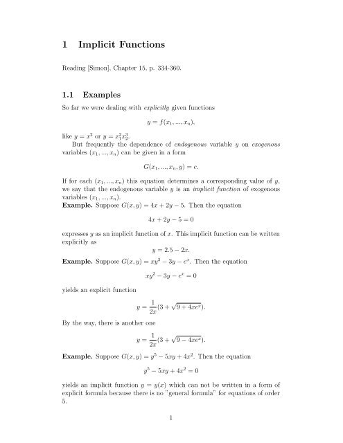
1 Implicit FunctionsReading [Simon], Chapter 15, p. 334-360.1.1 ExamplesSo far we were dealing with explicitly given functionsy = f(x 1 , ..., x n ),like y = x 2 or y = x 2 1x 3 2.But frequently the dependence of endogenous variable y on exogenousvariables (x 1 , ..., x n ) can be given in a formG(x 1 , ..., x n , y) = c.If for each (x 1 , ..., x n ) this equation determines a corresponding value of y,we say that the endogenous variable y is an implicit function of exogenousvariables (x 1 , ..., x n ).Example. Suppose G(x, y) = 4x + 2y − 5. Then the equation4x + 2y − 5 = 0expresses y as an implicit function of x. This implicit function can be writtenexplicitly asy = 2.5 − 2x.Example. Suppose G(x, y) = xy 2 − 3y − e x . Then the equationyields an explicit functionBy the way, there is another onexy 2 − 3y − e x = 0y = 12x (3 + √ 9 + 4xe x ).y = 12x (3 + √ 9 − 4xe x ).Example. Suppose G(x, y) = y 5 − 5xy + 4x 2 . Then the equationy 5 − 5xy + 4x 2 = 0yields an implicit function y = y(x) which can not be written in a form ofexplicit formula because there is no ”general formula” for equations of order5.1

Example. Suppose G(x, y) = x 2 + y 2 − 1. The corresponding equationx 2 + y 2 − 1 = 0determines, as we know, the unit circle.It is evident that(x 1 = 0, y 1 = 1), (x 2 = 0, y 2 = −1), (x 3 = 1, y 3 = 0), (x 4 = −1, y 4 = 0)all lay on this circle, that is all four are particular solutions of this equations.1. Around (x 1 = 0, y 1 = 1) this equation determines the explicit functiony = √ 1 − x 2 ,whose domain can be enlarged to x ∈ (−1, 1).2. Around (x 2 = 0, y 2 = −1) this equation determines the explicitfunctiony = − √ 1 − x 2 ,whose domain can be enlarged to x ∈ (−1, 1).3. Around (x 3 = 1, y 3 = 0) this equation determines the explicit functionx =√1 − y 2 ,whose domain can be enlarged to y ∈ (−1, 1).4. Around (x 4 = 1, y 4 = 0) this equation determines the explicit function√x = − 1 − y 2 ,whose domain can be enlarged to y ∈ (−1, 1).1.2 Implicit Function Theorem for R 2So our question is: Suppose a function G(x, y) is given. Consider the equationG(x 0 , y 0 ) = c.Does there exists a function y = y(x) defined on some interval (x 0 − ɛ, x 0 + ɛ)such that G(x, y(x)) ≡ c?OrDoes there exists a function x = x(y) defined in an interval (y 0 − ɛ, y 0 + ɛ)such that G(x(y), y) ≡ c?Such a function y = y(x) (or x = x(y)) is called implicit function definedby the equation G(x, y) = c around the point (solution) (x 0 , y 0 ). The graphof implicit function must be a locus the level curve G(x, y) = c.2

This picture shows that y(x) does not exist around the point A of thelevel curve G(x, y) = c (note that x = x(y) does not exist around D).Why so? What is wrong, with A? Because around A the level curveG(x, y) = c can not pass the vertical line test (the horizontal line test for D).Note that the tangent line at A is vertical, and this means that the gradientat A is horizontal, and this means that G y (A) = 0. This is wrong with A!And what is wrong with D?Theorem 1 Suppose a point (x ∗ , y ∗ ) ∈ R 2 is a particular solution of G(x ∗ , y ∗ ) =c and ∂G∂y (x∗ , y ∗ ) ≠ 0. Then the equationG(x, y) = cdetermines the function y = y(x) defined on some interval I = (x ∗ −ɛ, x ∗ +ɛ)about the point x ∗ such that(a) G(x, y(x)) ≡ c for all x ∈ I;(b) y(x ∗ ) = y ∗ ;(c) y ′ (x ∗ ) = − ∂G∂x (x∗ ,y ∗ ).∂G∂y (x∗ ,y ∗ )Proof. We prove the implication (a), (b) ⇒ (c). So, suppose we havey(x) such that y(x ∗ ) = y ∗ and G(x, y(x)) = c for all x ∈ I. DifferentiatingG(x, y(x)) = c with respect to x at x ∗ we obtainorand this gives (c).∂G∂x (x∗ , y(x ∗ )) · dxdx + ∂G∂y (x∗ , y(x ∗ )) · dydx (x∗ ) = 0,∂G∂x (x∗ , y ∗ ) + ∂G∂y (x∗ , y ∗ ) · y ′ (x ∗ ) = 0,In fact this Theorem states that may be y can not be solved as anfunction of x explicitly but it is possible to find the derivative y ′ (x ∗ )3

Let as check G z = 8xz − 6yzG z (0.5, 0, 0.6614378278) = 2.645751311 ≠ 0,G z (0.5, 0, −0.6614378278) = −2.645751311 ≠ 0,so it both cases - it does.Now we compute z x and z y at this point:andz x (0.5, 0, 0.6614378278) = − GxG z(0.5, 0, 0.6614378278),− G x(0.5,0,0.6614378278)= − 2.500000000 = 0.9449111825.G z (0.5,0,0.6614378278) −2.645751311z y (0.5, 0, 0.6614378278) = − G yG z(0.5, 0, 0.6614378278),− G y(0.5,0,0.6614378278)= − −2.500000000 = −0.4960783708.G z(0.5,0,0.6614378278) −1.312500000Now we are ready to estimate the corresponding change in z if x increasesto 0.6 and y decreases to −0.2:∆z = z x · ∆x + z y · ∆y =0.944911182 · 0.1 + (−0.4960783708) · (−0.2) = 0.1937067924.Similarly for another solution (0.5, 0, −0.6614378278).Phhhhh!1.4 Regular PointsFor a given smooth enough function G(x, y) the equation G(x, y) = c definesthe smooth curve, the level curve. Suppose a point (x ∗ , y ∗ ) lays on this curve,i.e. is a solution of this equation.1. If for (x ∗ , y ∗ ) one has∂G∂y (x∗ , y ∗ ) ≠ 0then the locus of level curve G(x, y) = c around (x ∗ , y ∗ ) can be thought of asthe graph of a function y = y(x), and the slope of this curve is∂G∂x−(x∗ , y ∗ )∂G∂y (x∗ , y ∗ ) .2. If for (x ∗ , y ∗ ) one has∂G∂x (x∗ , y ∗ ) ≠ 0then the locus of level curve G(x, y) = c around (x ∗ , y ∗ ) can be thought of asthe graph of a function x = x(y), and the slope of this curve is∂G−∂y (x∗ , y ∗ )∂G∂x6(x ∗ , y ∗ ).

3. If for (x ∗ , y ∗ ) one has∂G∂y (x∗ , y ∗ ) ≠ 0and∂G∂x (x∗ , y ∗ ) ≠ 0then the locus of level curve G(x, y) = c around (x ∗ , y ∗ ) can be thought of asthe graph of a function y = y(x) and y = y(x), and the slope of this curveat (x ∗ , y ∗ ) with respect to x axis is:∂G∂x−(x∗ , y ∗ )∂G∂y (x∗ , y ∗ )and the slope of this curve with respect to y axis is:∂G∂y−(x∗ , y ∗ )∂G∂x (x∗ , y ∗ ) .(What? We have two different slopes for one curve? Explain).Definition 1 A point (x ∗ , y ∗ ) is called regular point of G(x, y) if∂G∂x (x∗ , y ∗ ) ≠ 0, or ∂G∂y (x∗ , y ∗ ) ≠ 0.If every point of G(x, y) = c is regular, then the level set G(x, y) = c is calleda regular curve.So the Implicit Function Theorem states that at each point of regularcurve we can consider y as a function of x or x as a function of y.Example. Consider G(x, y) = x 2 , you know the graph of this function.Its level curve G(x, y) = 0 is just the y-axes: G(x, y) = x 2 = 0 ⇒ x =0. Each point of this level curve (0, y) is irregular: G x (0, y) = (2x)| 0,y) =0, G y (0, y) = 0| (0,y) = 0 (nevertheless this curve determines implicit functionx(y) = 0).1.5 Tangent of the Level CurveTheorem 3 The tangent vector to the level curve G(x ∗ , y ∗ ) = c at a regularpoint (x ∗ , y ∗ ) is(G y (x ∗ , y ∗ ), −G x (x ∗ , y ∗ )).7

Proof. Recall that the tangent vector of a curve (x(t), y(t)) is (x ′ (t), y ′ (t)).Suppose G(x ∗ , y ∗ ) = c and G y (x ∗ , y ∗ ) ≠ 0, then there exists implicitfunction y = y(x) around x ∗ , i.e. G(x, y(x)) = c. Thus this level curve isgiven by (x, y(x)) locally around x ∗ . Then its tangent vector at (x ∗ , y ∗ ) isgiven by(x ′ , y ′ (x)) = (1, − G x(x ∗ , y ∗ )G y (x ∗ , y ∗ ) ),this vector is parallel to (G y (x ∗ , y ∗ ), −G x (x ∗ , y ∗ )).Corollary 1 At a regular point the gradient is orthogonal to level curve.Proof.∇G(x ∗ , y ∗ ) · (G y (x ∗ , y ∗ ), −G x (x ∗ , y ∗ ) =(G x (x ∗ , y ∗ ), G y (x ∗ , y ∗ ) · (G y (x ∗ , y ∗ ), −G x (x ∗ , y ∗ ) =G x (x ∗ , y ∗ ) · G y (x ∗ , y ∗ ) − G y (x ∗ , y ∗ ) · G x (x ∗ , y ∗ ) = 0.Important Example. Let F (x, y) = x 2 + y 2 and G(x, y) = x · y. Finda point (x ∗ , y ∗ ) on the level curve G(x, y) = 1 and c such that the curvesG(x, y) = 1 and F (x, y) = c touch each other at the point (x ∗ , y ∗ ).Solution. The slope of tangent line of G(x, y) = 1 at (x ∗ , y ∗ ) is− G x(x ∗ , y ∗ )G y (x ∗ , y ∗ )and the slope of tangent line of F (x, y) = c at (x ∗ , y ∗ ) is− F x(x ∗ , y ∗ )F y (x ∗ , y ∗ ) .So we can find (x ∗ , y ∗ ) from the system of equations⎧⎪⎨G x (x ∗ ,y ∗ )= F x(x ∗ ,y ∗ )G y (x ∗ ,y ∗ ) F y (x ∗ ,y ∗ )⎪⎩G(x ∗ , y ∗ ) = 1which in our case looks as⎧⎪⎨⎪⎩y ∗x ∗= 2x∗2y ∗x ∗ · y ∗ = 1.The solution gives (x ∗ = 1, y ∗ = 1) and (x ∗ = −1, y ∗ = 1). In both casesc = F (1, 1) = F (−1, −1) = 2.8

of a utility function and the slope of an isoquant of a production function,since in these situations we are interested in which directions to move to keepthe function constant.The level curve of a utility function U(x, y) is called an indifference curveof U.Its slope at (x ∗ , y ∗ ) is called the marginal rate of substitution (MRS) ofU at (x ∗ , y ∗ ) since it measures, in a marginal sense, how much more of goody the consumer would require to compensate for the loss of one unit of goodx to keep the same level of satisfaction.By the Implicit Function Theorem, the MRS at (x ∗ , y ∗ ) is:∂U∂x−(x∗ , y ∗ )∂U∂y (x∗ , y ∗ )Similarly, if Q = F (K, L) is a production function, its level curves are calledisoquants and the slope - F K /F L of an isoquant at (Ko, Lo) is called themarginal rate of technical substitution (MRTS). It measures how much ofone input would be needed to compensate for a one-unit loss of the otherunit while keeping production at the same level.Example. Consider a function f(x, y) = x 2 e y .(a) What is the slope of the level set at x = 2, y = 0?(b) In what direction should one move from the point (2, 0) in order toincrease f most quickly? Express your answer as a vector of length 1.(c) Suppose at (2, 0) the variable x is changed to 2.5. Estimate thecorresponding change of y = 0 which substitutes this change of x, that isthe output remains the same.Solution.thus∂f∂x (x, y) = 2xey ,∂f∂f(2, 0) = 4,∂x∂f∂y (x, y) = x2 e y ,(2, 0) = 4.∂y(a) So the slope of the level curve at (2, 0) is −1.(b) The function f increases most rapidly in the direction of gradient∇f(2, 0) = (4, 4).The suitable vector of the length 1 is ( 1 √2,1 √2 ).(c) f(2 + ∆x, 0 + ∆y) − f(2, 0) ≈ ∂f∂x= 4 · 0.5 + 4 · ∆y = 0, ∆y = −0.5.The same using MRS:∂f(2, 0) · ∆x + (2, 0) · ∆y∂y∆y∆x ≈ MRS = −f x(2, 0)f y (2, 0) = −4 4 = −1,thus ∆y = MRS · ∆x = −1 · ∆x = −0.510

1.7 System of Implicit FunctionsFirst warming up. Start with a system of linear equations⎧⎪⎨⎪⎩a 11 x 1 + ... + a 1n x n + b 11 y 1 + ... + b 1m y m = c 1a 21 x 1 + ... + a 2n x n + b 21 y 1 + ... + b 2m y m = c 2... ... ... ... ... ... ... ... ... ... ... ... ...a m1 x 1 + ... + a mn x n + b m1 y 1 + ... + b mm y m = c mIs it possible to express the (endogenous) variables y 1 , y 2 , ... , y m in terms of(exogenous) variables x 1 , x 2 , ... x n ? Answer is ”yes” if⎛⎜det ⎝⎞b 11 ... b 1m⎟... ... ... ⎠ ≠ 0.b m1 ... b mmNow turn to general problem. Suppose m functions F i (x 1 , ..., x n , y 1 , ..., y m ), i =1, ..., m, (i.e. F i : R n+m → R, i = 1, ..., m) are given. We consider a systemof equations ⎧⎪⎨ F 1 (x 1 , ..., x n , y 1 , ..., y m ) = c 1................, (1)⎪ ⎩F m (x 1 , ..., x n , y 1 , ..., y m ) = c mand suppose a point (x ∗ 1, ..., x ∗ n, y ∗ 1, ..., y ∗ m) ∈ R n+m is a solution.(a) Does there exist functions y 1 (x 1 , ..., x n ), ... , y m (x 1 , ..., x n ) in someneighborhood of x ∗ = (x ∗ 1, ..., x ∗ n) such thatF i (x 1 , ..., x n , y 1 (x 1 , ..., x n ), ..., y m (x 1 , ..., x n )) ≡ c i , i = 1, ..., m,and y i (x ∗ 1, ..., x ∗ n) = y ∗ i , i = 1, ..., m?(b) How to compute partial derivatives ∂y i∂x j(x ∗ 1, ..., x ∗ n)?Theorem 4 If the determinant of Jacobian matrix⎛⎜⎝∂F 1∂y 1...∂F 1∂y m... ... ...∂F m∂y 1...∂F m∂y mevaluated at (x ∗ 1, ..., x ∗ n, y ∗ 1, ..., y ∗ m) is nonzero, then there exist functions⎞⎟⎠y 1 (x 1 , ..., x n ), ... , y m (x 1 , ..., x n )defined on a ball about (x ∗ 1, ..., x ∗ n) satisfying the conditionsF i (x 1 , ..., x n , y 1 (x 1 , ..., x n ), ..., y m (x 1 , ..., x n )) ≡ c i , i = 1, ..., m,and y i (x ∗ 1, ..., x ∗ n) = y ∗ i , i = 1, ..., m.11

Furthermore, the derivatives ∂y i∂x kcan be solved from the system of linearequations⎛ ∂F 1 ∂F∂y⎜ 1... 1⎞ ⎛ ⎞∂y 1⎛ ∂F 1⎞∂y m⎟∂x k⎝ ... ... ... ⎠ · ⎜⎝ ... ⎟⎠ = − ∂x⎜ k⎟⎝ ... ⎠ . (2)∂F m ∂F∂y 1... 1 ∂y m∂F m∂y m ∂x k∂x kThe solution of this system can be computed by⎛⎜⎝∂y 1∂x k...∂y m∂x k⎞ ⎛⎟⎠ = − ⎜⎝∂F 1∂y 1...∂F 1∂y m... ... ...∂F m∂y 1...∂F 1∂y m⎞−1⎟⎠·⎛⎜⎝∂F 1∂x k...∂F m∂x kor by Cramer’s rule (Here all the matrices evaluated at (x ∗ 1, ..., x ∗ n, y ∗ 1, ..., y ∗ m)).Sketch of Proof. Let us differentiate our system (1) by x k :⎧⎪⎨⎪⎩∂F 1∂x k+ ∂F 1∂y 1· ∂y 1∂x k+ ... + ∂F 1∂y m· ∂ym∂x k= 0∂F 2∂x k+ ∂F 2∂y 1· ∂y 1∂x k+ ... + ∂F 2∂y m· ∂ym∂x k= 0... ... ... ... ... ... ... ... ...∂F m∂x k+ ∂F m∂y 1· ∂y 1∂x k+ ... + ∂F m∂y m· ∂ym∂x k= 0and this system is exactly (2).Example. One solution of the systemx 3 y − z = 1x + y 2 + z 3 = 6is (x = 1, y = 2, z = 1). Estimate the corresponding x and y when z = 1.1.Solution. Take F 1 (x, y, z) = x 3 y − z, F 2 (x, y, z) = x + y 2 + z 3 .Evaluating the whole Jacobian at (x = 1, y = 2, z = 1) we obtain( ∂F1∂x∂F 2∂x∂F 1∂y∂F 2∂y∂F 1∂z∂F 2∂zThe determinant ∣ ∣∣∣∣ ∂F 1)∂x∂F 2∂x=∂F 1∂y∂F 2∂y⎞⎟⎠(3x 2 y x 3 ) (−1 6 1 −11 2y 3z 2 =1 4 1∣ ∣∣∣∣ ∣ = 6 1= 23 ≠ 0,1 4 ∣so the Implicit Function Theorem asserts the existence of a solution x(z) andy(z) as functions of exogenous variable z.Now calculate derivatives x ′ (1) = x z (1) and y ′ (1) = y z (1):( ∂F1∂x∂F 2∂x∂F 1∂y∂F 2∂y)·(x ′ (1)y ′ (1))=(−∂F 1∂z− ∂F 2∂z),).12

evaluating we obtain a system of linear equations(6 11 4)·(x ′ (1)y ′ (1))=(1−3and the solution gives x ′ (1) = 7 , 23 y′ (1) = −19.23Now we are ready to estimate x(1.1) and y(1.1) by linear approximation:x(1.1) ≈ x(1) + x ′ (1) · 0.1 = 1 + 7 0.1 = 1.03,23y(1.1) ≈ y(1) + y ′ (1) · 0.1 = 2 + −19 0.1 = 1.91.23Finally we obtain the estimation of new solution (x = 1.03, y = 1.91, z = 1.1).Example. For the systemxz 3 + y 2 v 4 = 2, xz + yvz 2 = 2(x = 1, y = 1, z = 1, v = 1) is a solution.(a) Can you estimate a new solution which correspond to y = 1.1 andv = 1.2?(b) Can you estimate a new solution which correspond to x = 1.1 andy = 1.2?Solution. Take F 1 (x, y, z) = xz 3 + y 2 v 4 , F 2 (x, y, z) = xz + yvz 2 .Evaluating the whole Jacobian at (x = 1, y = 1, z = 1, v = 1) we obtain( ∂F1∂x∂F 2∂x∂F 1∂y∂F 2∂y∂F 1∂z∂F 2∂z∂F 1∂v∂F 2∂v)(1,1,1,1)(z32yv=4 3xz 2 4y 2 v 3 )z vz 2 x + 2yvz yz 2( )1 2 3 4.1 1 3 1),(1,1,1,1)=(a) The determinant∂F 1∂x∣ ∂F 2∂x∂F 1∂z∂F 2∂z=∣ ∣(1,1,1,1)1 31 3∣ = 0,so the Implicit Function Theorem does not alow to express x and z as functionsof Y and v.(b) The determinant∂F 1∂z∣ ∂F 2∂z∂F 1∂v∂F 2∂v=∣ ∣(1,1,1,1)3 43 1= −9 ≠ 0,∣so the Implicit Function Theorem asserts the existence of solutions z(x, y)and v(x, y) as functions of exogenous variables x and y.Now we calculate derivatives z x , z y , v x , v y at (1, 1, 1, 1).13

For z x and v x we have the system( ∂F1∂z∂F 2∂z∂F 1∂v∂F 2∂v)·(zx (1, 1)v x (1, 1)evaluating we obtain a system of linear equations(3 43 1)·(zx (1, 1)v x (1, 1)))==(−∂F 1∂x− ∂F 2∂x(−1−1),),and the solution gives z x (1, 1) = −13 , v x(1, 1) = 0.Similarly, for z y and v y we have the system( ∂F1∂z∂F 2∂z∂F 1∂v∂F 2∂v)·(zy (1, 1)v y (1, 1))=( −∂F 1∂y− ∂F 2∂y),evaluating we obtain a system of linear equations(3 43 1)·(zy (1, 1)v y (1, 1))=(−2−1and the solution gives z y (1, 1) = −29 , v x(1, 1) = −1.),14

2 Inverse Function*Suppose f : X → Y is a function from X to Y . This function is calledinvertible if there exists the inverse function g : Y → X such thatg(f(x)) = x and f(g(y)) = yfor each x ∈ X and y ∈ Y . In other words the composition g ◦ f coincideswith the identity map id X : X → X and the composition f ◦g coincides withthe identity map id Y : Y → Y .Examples1. The map f : R → R given by f(x) = 2x + 4 is invertible and it’sinverse is the map g : R → R given by g(y) = 0.5y − 2. Indeed,andg(f(x)) = g(2x + 4) = 0.5(2x + 4) − 2 = x,f(g(y)) = f(0.5y − 2) = 2(0.5y − 2) + 4 = y.2. The map f : R → R + = (0, +∞) given by f(x) = e x is invertible andit’s inverse is the map g : R + → R given by g(y) = ln y. Indeed,g(f(x)) = g(e x ) = ln e x = x, and f(g(y)) = f(ln y) = e ln y = y.A map f : X → Y is called surjective if for each y ∈ Y there exists x ∈ Xs.t. f(x) = y.A map f : X → Y is called injective if for x 1 ≠ x 2 we have f(x 1 ) ≠ f(x 2 ).A map f : X → Y is called bijective if it is surjective and injectivesimultaneously.Let us interpret these notions in terms of equationf(x) = ywhere x is considered as an unknown.A map f : X → Y is surjective iff the equation f(x) = y has a solutionfor each y ∈ Y .A map f : X → Y is injective iff the equation f(x) = y has either nosolution or unique solution for each y ∈ Y .A map f : X → Y is bijective iff the equation f(x) = y has uniquesolution for each y ∈ Y .Theorem 5 A map f : X → Y is invertible if and only if it is a bijection.15

2.1 Invertible Linear mapsA linear map F : R n → R n in fact is given by a matrix⎛A = ⎜⎝and F (v) = A · v for each vector v ∈ R n .⎞a 11 a 12 ... a 1na 21 a 22 ... a 2n⎟... ... ... ... ⎠a m1 a m2 ... a mnTheorem 6 A linear map F : R n → R n is invertible if and only if it’smatrix A is nondegenerate, that is det A ≠ 0. In this case the inverse mapG : R n → R n is given by G(w) = A −1 · w.2.2 Inverse Function TheoremSuppose now F : R n → R n is function. As we know such a function is acollection of functionsf 1 : R n → Rf 2 : R n → R...f n : R n → R,so thatF (x 1 , ..., x n ) = (f 1 (x 1 , ..., x n ), f 2 (x 1 , ..., x n ), ..., f n (x 1 , ..., x n )).The matrix which consists of partial derivatives of these functionsDF =⎛⎜⎝∂f 1∂f 1∂x n∂x 1...... ... ...∂f n∂x 1...is called Jacobian of F . By DF (x ∗ ) is denoted the numerical matrix obtainedby evaluation of Jacobian DF at a vector x ∗ = (x ∗ 1, ..., x ∗ n).Theorem 7 Suppose F (x ∗ ) = y ∗ and the Jacobian DF (x ∗ ) is nondegeneratematrix, then there exists an open ball B r (x ∗ ) about x and an open set U ⊂ R nabout y ∗ such that the restriction of the map FF : B r (x ∗ ) → Uis invertible (this is called locally invertible). Furthermore, the jacobianof inverse mapG = F −1 : U → B r (x ∗ )is the inverse matrix of the Jacobian of F :∂f n∂x n⎞⎟⎠DG(y ∗ ) = (DF (x ∗ )) −1 .16

Example. Consider the function F : R 2 → R 2 given byIt’ Jacobian looks asF (x, y) = (x 2 − y 2 , 2xy).( )2x −2yDF =2y 2xand its determinant is detDF (x, y) = 4(x 2 + y 2 ). By the Inverse FunctionTheorem, F is locally invertible at every point except (0, 0).Example. Show that the map F (x, y) = (x + e y , y + e −x ) is everywherelocally invertible.Solution. The Jacobian looks as( )1 eyDF =−e −x 1so it’s determinant is 1 + e y−x . This expression is nonzero at any (x, y).17

Exercises1. Consider the equation x 3 + 3y 2 + 4xz 2 − 3z 2 y = 1. Does this equationdefine z as a function of x and y:(a) In a neighborhood of x = 1, y = 1?(b) In a neighborhood of x = 1, y = 0?(c) In a neighborhood of x = 0.5, y = 0?If so, compute ∂z∂xand∂z∂yat that point.2. Consider the function F (x 1 , x 2 , y) = x 2 1 − x 2 2 + y 3 .(a) If x 1 = 6 and x 2 = 3, find a y which satisfies F (x 1 , x 2 , y) = 0.(b) Does this equation define y as an implicit function of x 1 and x 2 nearx 1 = 6, x 2 = 3?(c) If so, compute ∂y∂x 1(6, 3) and ∂y∂x 2(6, 3)(d) If x 1 increases to 6.2 and x 2 decreases to 2.9, estimate the correspondingchange of y.3. Show that if for functions f(x, y) and g(x, y) one has f x = g y andf y = −g x , then level curves of f and g intersect orthogonally.4. One solution of the system2x 2 + 3xyz − 4uv = 16,x + y + 3z + u − v = 10is x = 1, y = 2, z = 3, u = 0, v = 1. If one varies u and v near their originalvalues and plugs these new values into this system, can one find unique valuesof x, y and z that still satisfy this system? Explain.5. Check that x = 1, y = 4, u = 1, v = −1 is a solution of the systemy 2 + 2u 2 + v 2 − xy = 15, 2y 2 + u 2 + v 2 + xy = 38.If y increases to 4.02 and x stays fixed, does there exist a (u, v) near (1, −1)which solves this system? If not, why not? If yes, estimate the new u and v.6. The economy of Northern Saskatchewan is in equilibrium when thesystem of equations2xz + xy + z − 2 √ z = 11, xyz = 6is satisfied. One solution of this set of equations is x = 3, y = 2, z = 1,and Northern Saskatchewan is in equilibrium at this point. Suppose that the18

prime minister discovers that the variable z (output of beaver pelts) can becontrolled by simple decree.a) If the prime minister raises z to 1.1, use calculus to estimate the changein x and y.b) If x were in the control of the prime minister and not y or z, explainwhy you cannot use this method to estimate the effect of reducing x from 3to 2.95.7. Consider the system of equationsx + 2y + z = 5, 3x 2 yz = 12as defining some endogenous variables in terms of some exogenous variables.a) Divide the three variables into exogenous ones and endogenous ones ina neighborhood of x = 2, y = 1, z = 1 so that the Implicit Function Theoremapplies.b) If each of the exogenous variables in your answer to a) increases by 0.25,use calculus to estimate how each of the endogenous variables will change.8. Consider the system of two equations in three unknowns: x + 2y + z =5, 3x 2 yz = 12.a) At the point x = 2, Y = 1, z = 1, why can we treat z as an exogenousvariable and x and y are the dependent variables?b) If z rises to 1.2, use calculus to estimate the corresponding x and y.Exercises 15.1-15.25 from [SB].HomeworkExercise 15.6 from [SB], Exercise 15.9 from [SB], Exercise 15.13 from [SB],Exercise 15.22 from [SB], Exercise 15.24 from [SB].19

Short SummaryImplicit FunctionImplicit Function Theorem in R 1 If G(x ∗ , y ∗ ) = c and ∂G∂y (x∗ , y ∗ ) ≠ 0,then ∃ y = y(x) on (x ∗ − ɛ, x ∗ + ɛ) s.t. G(x, y(x)) ≡ c, y(x ∗ ) = y ∗ andy ′ (x ∗ ) = − ∂G∂x (x∗ ,y ∗ ).∂G∂y (x∗ ,y ∗ )Implicit Function Theorem for R n . If G(x ∗ 1, ..., x ∗ k, y ∗ ) = c and∂G∂y (x∗ 1, ..., x ∗ k, y ∗ ) ≠ 0then ∃ y = y(x 1 , ..., x n ) on B ɛ (x ∗ ) s.t. G(x 1 , ..., x k , y(x 1 , ..., x k )) ≡ c,y(x ∗ 1, ..., x ∗ k) = y ∗ and ∂y∂x i= − ∂G (x ∂x ∗ i1 ,...,x∗ k ,y∗ ).∂G∂y (x∗ 1 ,...,x∗ k ,y∗ )Implicit Function Theorem for System. If⎧⎪⎨⎪⎩F 1 (x ∗ 1, ..., x ∗ n, y1, ∗ ..., ym) ∗ ⎞= c 1................F m (x ∗ 1, ..., x ∗ n, y1, ∗ ..., ym) ∗ = c m⎟⎠ and∣∂F 1∂y 1...∂F 1∂y m... ... ...∂F m∂y 1...∂F m∂y m∣ ∣∣∣∣∣∣(x ∗ 1 ,...,x∗ n ,y∗ 1 ,...,y∗ m ) ≠ 0,then ∃ y 1 (x 1 , ..., x n ), ... , y m (x 1 , ..., x n ) on B ɛ (x ∗ , Y ∗ ) s.t. for all i = 1, ..., mF i (x 1 , ..., x n , y 1 (x 1 , ..., x n ), ..., y m (x 1 , ..., x n )) ≡ c i ,y i (x ∗ 1, ..., x ∗ n) = y ∗ iand ∂y i∂x kcan be solved from⎛⎜⎝∂F 1∂y 1...∂F 1∂y m... ... ...∂F m∂y 1...∂F 1∂y m⎞⎟⎠ ·⎛⎜⎝∂y 1∂x k...∂y m∂x k⎞ ⎛⎟⎠ = − ⎜⎝Regular point of G(x, y): DG(x ∗ , y ∗ ) ≠ (0, 0).∂F 1∂x k...∂F m∂x kTangent vector of the level curve G(x, y) = c at a regular point(x ∗ , y ∗ ): (G y (x ∗ , y ∗ ), −G x (x ∗ , y ∗ )).⎞⎟⎠ .At a regular point gradient is orthogonal to level curve.Marginal Rate of Substitution ∆y ≈ MRS · ∆x = − ∂G∂x (x∗ ,y ∗ )∂G∂y (x∗ ,y ∗ ) ∆x.20