The water footprint and virtual water exports of Spanish tomatoes

Papeles de Agua VirtualThe water footprint andvirtual water exportsof Spanish tomatoesD. ChicoG. SalmoralM.R. LlamasA. GarridoM.M. AldayaNúmero 8

PAPELES DE AGUA VIRTUALNúmero 8THE WATER FOOTPRINT ANDVIRTUAL WATER EXPORTSOF SPANISH TOMATOESD. Chico 1 , G. Salmoral 1 , M.R. Llamas 2 ,A. Garrido 1 and M.M. Aldaya 1,31CEIGRAM, Universidad Politécnica de Madrid, Spain2Departamento de Geodinámica, Universidad Complutense de Madrid,Spain3Twente Water Centre, University of Twente, Enschede, The Netherlandshttp://www.fundacionmbotin.org

Papeles de Agua Virtual. Observatorio del AguaEdita: Fundación Marcelino Botín. Pedrueca, 1 (Santander)www.fundacionmbotin.orgISBN: 978-84-96655-23-2 (obra completa)ISBN: 978-84-96655-80-5 (Número 8)Depósito legal: M. 51.649-2010Impreso en REALIGRAF, S.A. Madrid, noviembre de 2010

TABLE OF CONTENTSSUMMARY .................................................................. 51. INTRODUCTION ................................................ 62. METHOD AND DATA ........................................ 92.1. Water footprint calculation of tomato productionin open-air systems........................ 102.2. Water footprint calculation of tomatogreenhouse production ................................ 162.3. Calculation of the water apparent productivityand exported virtual water............... 183. THE WATER FOOTPRINT OF 1 KILOGRAMOF TOMATOES................................................... 203.1. Aggregated water footprint......................... 203.2. Disaggregated water footprint: Analysisbetween production systems....................... 244. APPARENT WATER PRODUCTIVITY ANDVIRTUAL WATER EXPORTS OF TOMATOPRODUCTION..................................................... 284.1. Water apparent productivity of tomatoproduction..................................................... 284.2. Water apparent productivity of surface orgroundwater ................................................. 314.3. Virtual water exports.................................. 335. DISCUSSION....................................................... 346. CONCLUSION..................................................... 40

4 THE WATER FOOTPRINT OF TOMATO PRODUCTION7. ACKNOWLEDGEMENTS .................................. 419. REFERENCES..................................................... 4210. APPENDIX........................................................... 49

THE WATER FOOTPRINT AND VIRTUALWATER EXPORTS OF SPANISH TOMATOESD. Chico 1 , G. Salmoral 1 , M.R. Llamas 2 ,A. Garrido 1 and M.M. Aldaya 1,31CEIGRAM, Universidad Politécnica de Madrid, Spain2Departamento de Geodinámica, UniversidadComplutense de Madrid, Spain3Twente Water Centre, University of Twente,Enschede, The NetherlandsSUMMARYThe water footprint is an indicator of water use that looksat both direct and indirect water use of a consumer or aproducer. The present study analyses the green, blue andgrey water footprint of tomato production in Spain. It assessesthe water apparent productivity between differentproduction systems and seasons. It also compares the productivitiesof surface and groundwater and evaluates thevirtual water of tomato exports. The total water footprintof 1 kilogram of tomatoes produced in Spain is about 236litres per kilogram as a national average, ranging from 216to 306 litres per kilogram. The water footprint of freshtomatoes varies in the different locations mainly dependingon the local agro-climatic character, total tomato productionvolumes and production systems. The Spanish averagegreen water footprint component amounts to about 5%, theblue component 36% and the grey component 59%. The differencesin the water footprint between production systems

6 THE WATER FOOTPRINT OF TOMATO PRODUCTIONare notable (open-air - rainfed or irrigated- versus greenhouse).Rainfed open-air tomato production has by far thehighest water footprint with 966 l/kg, of which 84% is greywater footprint. The grey footprint of irrigated systems is,in comparison to that of rainfed systems, much lower, mainlydue to the higher yields of these production systems. Themajor producing provinces in Spain have in general low waterfootprints in terms of l/kg compared to the average ofthe rest of the provinces, but a much higher total water footprintin absolute terms (hm 3 ). This is because theseprovinces produce overwhelmingly the most part of the nationalproduction. The green and blue water apparent productivityof the tomato production ranged from 2.1 €/m 3 forrainfed systems to 3.1 €/m 3 of open-air irrigated systemsand 7.8 €/ m 3 for greenhouse production. By season, tomatoproduced in the middle season (June to September) renderedthe lowest apparent water productivity with 2.7 €/m 3 .By contrast, tomatoes produced in early (January to May)or late season (September to December) rendered higher apparentwater productivities, 7.5 and 9.5 €/l respectively. Inrelation to the origin of water, groundwater production presenteda higher blue water apparent productivity than thatof open-air irrigated production, around 7 €/m 3 compared to3 €/m 3 . When analysing the exports of tomato the yearlyamount of virtual water exported through the tomato exportsis 4, 88 and 134 hm 3 of green, blue and grey water respectively,with an average water apparent productivity of8.81 €/m 3 .1. INTRODUCTIONIn a context where water resources are unevenly distributedand, in regions where flooding and drought risks maybecome more severe, enhanced water management is a majorchallenge not only to water users and managers but also

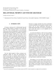
D. CHICO et al. 7to final consumers, businesses and policymakers in general.From a global perspective, about 86% of all water is usedto grow food (Hoekstra and Chapagain, 2008). Parallel tothis, food choices can have a big impact on water demand.From the production perspective, agriculture has to competewith other water users like the environment, municipalitiesand industries (UNESCO, 2006).In Spain, tomato production represents 5% of the grossnational agricultural production with a yearly average productionof about 4 million tons in 62,939 ha. In economicterms, tomato production represents a 6.6 % of the gross nationalagricultural production in the study period (MARM,2010b). Of this production, around 25% is exported eachyear, mainly to the European Markets as fresh tomato(Reche, 2009). Tomato production in Spain represents 1.5%of the total Spanish water footprint (Garrido et al., 2010).The main producing areas are the Guadiana Valley in southwestSpain, and the southeast corner in the provinces ofAlmería, Murcia and Granada (Figure 1). These two regionsare quite different in their production methods. The Guadianavalley produces almost exclusively open-air, irrigatedtomatoes (Campillo, 2007) for the food industry (i.e. inputfor tomato sauce and powder transformation), using surfacewater from the Guadiana valley (CHG, 2008; Aldaya andLlamas, 2009), whereas the southeast region, mainly thecoastal plain of Almería province, has developed the highestconcentration of greenhouses in a particular area of theworld (Castilla, 2009). Its dynamic production has evolvedfrom primary greenhouses to more complex and developedgrowing systems that produce high quality horticulturalcrops for export throughout the year (García 2009), almostexclusively out of groundwater (Regional Government of Andalusia2003). Along these two regions, tomato productionwas traditionally significant in other parts of the country,where, although declining, tomato production is still impor-

8 THE WATER FOOTPRINT OF TOMATO PRODUCTIONFIGURE 1. Tomato producing provinces with the proportion of productionand system in each province. The size of the pie charts is proportional tothe annual production of the provinceSource MARM (2009).tant. These regions include the Canary Islands, the Mediterraneancoast (Alicante, Valencia, Castellón and Balearesprovinces) and the Ebro valley. In these areas, especially inthe Canary Islands and the Ebro valley, this crop has a significantimportance for the regional economy (Maroto, 2002;Suárez, 2002).The concept of the ‘water footprint’ has been proposed asan indicator of water use that looks at both direct and indirectwater use of a consumer or producer (Hoekstra,2003). The water footprint is a comprehensive indicator offreshwater resources use, complementary to measures of directwater withdrawal. The water footprint of a product is

D. CHICO et al. 9the volume of freshwater used to produce the product, measuredalong the full supply chain. It is a multi-dimensionalindicator, showing water consumption volumes by sourceand polluted volumes by type of pollution; all componentsof a total water footprint are specified geographically andtemporally (Hoekstra et al., 2009). The blue water footprintrefers to consumption of blue water resources (surface andgroundwater) along the supply chain of a product. ‘Consumption’refers to loss of water from the available groundsurfacewater body in a catchment area. This fraction thatevaporates is incorporated into a product, or returns to anothercatchment area. The green water footprint refers toconsumption of green water resources (rainwater stored inthe soil as soil moisture). The grey water footprint refers topollution and is defined by the volume of freshwater thatis required to assimilate the load of pollutants to meet existingambient water quality standards.The present study analyses the water footprint of tomatoproduction in Spain. In particular, it focuses on the green,blue (surface and groundwater) and grey water footprint oftomato production in the different Spanish provinces. Differenttypes of tomato production systems are analysed:open-air (irrigated and rainfed) and greenhouse. For eachof them, the respective water footprint was studied in thedifferent times of the year; early, middle and late season.To complete the analysis of the tomato sector with a socioeconomicperspective, evaluations of apparent water productivity(€/m 3 ) and virtual water exports of tomato are alsoreported.2. METHOD AND DATAThe present study estimates the green, blue and grey waterfootprint of 1 kilogram of tomato fruit produced in Spain

10 THE WATER FOOTPRINT OF TOMATO PRODUCTIONfollowing the method described by Hoekstra et al. (2009).In the study, the tomato production in the different Spanishprovinces was considered, distinguishing productionthroughout the year as well as between growing systems.The study focuses on the production stage, that is, the cultivationof the product, from sowing to harvest. The studyperiod selected was 1997-2008. The water footprint was calculatedfor each year distinguishing the green, blue andgrey water components.This study distinguishes the three water footprint components:green, blue and grey.WF = WF green+ WF blue+ WF greyE [1]in which:WF = the water footprint (litres/product).WF green= the green water footprint (litres /product).WF blue= the blue water footprint (litres /product).WF grey= the grey water footprint (litres /product).Due to the differences in growing system (open-air andcovered), the methodology for calculating the green and bluewater footprint will be presented separately. The methodologyfor calculating the grey water footprint was commonto both production systems.2.1. Water footprint calculation of tomatoproduction in open-air systemsThe water footprint of open-air tomato (rainfed or irrigated)has been calculated distinguishing the green and blueand grey water components. The green and blue water evap-

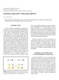
D. CHICO et al. 11otranspiration has been estimated using the CROPWATmodel (FAO, 1998; FAO, 2009a). Within this model, the ‘irrigationschedule option’ was applied, which includes a dynamicsoil water balance and keeps track of the soil moisturecontent over time. The calculations have been done usingclimate data from representative meteorological stations locatedin the major crop-producing provinces, selected dependingon data availability. Monthly reference evapotranspiration(ET o) and precipitation for each of the provinceswas obtained from the National Meteorological Agency(AEMET, 2010). When data were missing, it was completedwith the Integral Service Farmer Advice (MARM 2010a).The total crop area and production for each province wereobtained from the Agricultural and Statistics Yearbook foreach of the studied years, distinguishing growing systemsand growing periods (MARM, 2010b). In the case of the year2008, since data on seasonal production was not available,the same distribution as in 2007 was used. Data on plantingdates and growing length was taken from the “sowing andharvesting calendar” from the Ministry of the Environmentand Rural and Marine Affairs of Spain (MARM, 2002). Thisdatabase includes open-air and greenhouse production.However, when the data was markedly biased towardsshort growing length, or was missing, the data was adjustedfrom that of the nearest, agronomically similar province(Appendix I).Crop parameters required for the evapotraspiration calculationwere based on FAO (1998), adjusted when more localinformation was found (Campillo, 2007) (Table 1).Data on soil types was taken from the EUROSTAT soilmap (CEC, 1985) at 1:1,000,000 scale. Textural classes wereused to determine the soil characteristics and were classifiedin four categories: Sandy-Loam, Loam, Clay-Loam andClay. Canary Islands’ textural classes are based on the Dig-

12 THE WATER FOOTPRINT OF TOMATO PRODUCTIONTABLE 1. Crop parameters used for the estimation of the tomatoevapotranspiration in SpainInitialMiddle FinalDevelopmentStage stage stageKc 0.6 1.25 0.8Root depth (m) 0.1 0.5Critical Depletion 0.3Crop height2 mSource: FAO (1998), Nuez (1995).ital Soil Map of the World (FAO-UN, 2007) at 1:5,000,000scale. For each province the most frequent soil texture wasapplied, which was obtained by overlaying the map of irrigatedareas and the soil texture map (Figure 2). The mapof irrigated areas was taken from the GIS service of theMinistry of Environment and Rural and Marine Affairs ofSpain (MARM, 2010c), which was contrasted with the maintomato producing regions in each province (Hoyos, 2005;Maroto, 2002; Nuez, 1995).In the case of irrigated production, crop blue water use(mm) was obtained selecting the “irrigate at fixed intervalper stage” and “refill soil to field capacity”options in theCROPWAT model considering thus an irrigation scheme thatcompletely satisfies the crop water demand. The actual evapotraspiration(Et a) during the entire growing period is partlyfulfilled by the rain and partly by irrigation. The blue waterevapotranspiration (ET blue) is equal to the ‘total net irrigation’as specified in the model. The green water evapotranspiration(ET green) of the crop is equal to the difference betweenthe total actual evapotraspiration and the net irrigation.ET ( irr= 1)= Total net irrigationblueE [2]ET ( irr= 1) = ET ( irr= i) − ET ( irr=1)greenablue

D. CHICO et al. 13FIGURE 2. Soil map of Spain with the different textural classesand irrigated areas sSource: Own elaboration based on EUROSTAT soil map (CEC, 1985) and MARM (2010b).Over the growing period, the blue water evapotranspirationis generally less than the actual irrigation volume applied.The difference refers to the irrigation water that percolatesto the groundwater or runs off from the field.Rainfed conditions can be simulated in the model bychoosing to apply no irrigation. In the rainfed scenario (irr= 0), the green water evapotranspiration is equal to the totalevapotranspiration as simulated by the model and theblue water evapotranspiration is zero:ET ( irr = 0)= 0blueE [3]

14 THE WATER FOOTPRINT OF TOMATO PRODUCTIONThe green water footprint of the crop (m 3 /ton) has beenestimated as the ratio of the green water use (m 3 /ha) to thecrop yield (ton/ha). The blue water footprint of the crop isassumed equal to the ratio of the volume of irrigation waterconsumed to the crop yield.WFWFgreenijklblue ijklET= ×10green ijklY10×ET=Y ijklijklblue ijklE [4]In which:i = year season (early, middle or late season).j = production system (rainfed, open-air irrigated or covered).k = province of the country.l = year of the study period (1997-2008).ET green ijkl= Green water evapotraspiration of the provincek, under the production system j in the yearseason i in the year l (mm).Y ijkl= Yield of the province k, under the production systemj in the year season i in the year l (t/ha).ET blue ijkl= Blue water evapotraspiration of the province k,under the production system j in the year seasoni in the year l (mm).Finally, the grey water footprint of a primary crop is anindicator of freshwater pollution associated with the productionof the crop (Hoekstra et al., 2009). It is defined asthe volume of freshwater that is required to assimilate theload of pollutants based on existing ambient water quality

D. CHICO et al. 15standards. The grey water footprint is calculated by dividingthe pollutant load (L, in mass/time) by the differencebetween the ambient water quality standard for that pollutant(the maximum acceptable concentration c max, inmass/volume) and its natural concentration in the receivingwater body (c nat, in mass/volume).WFblue ijklET= ×Y10 blue ijklijklE [5]As it is generally the case, the production of tomato concernsmore than one form of pollution. In our case though,the grey water footprint was estimated only for Nitrogen. Thetotal volume of water required to assimilate a ton of Nitrogenwas calculated considering the surplus Nitrogen, which endsup leaching. The natural concentration of Nitrogen in the receivingwater body was assumed negligible whereas the maximumallowable concentration in the ambient water systemconsidered was 50 mgNO 3-/l, as the concentration stated inthe EU Nitrates Directive (91/676/EEC). The pollutant loadconsidered was the excess Nitrogen based on data from theMinistry of the Environment and Rural and Marine Affairsof Spain (MARM, 2008) (Annex IV). This excess Nitrogenavailable for leaching or run-off (kg/ha) was then multipliedby the corresponding area in order to obtain the total load ofNitrogen (kg) reaching the surface or groundwater systems.This was divided by the ambient water quality standard andthe corresponding crop yield (ton/ha) to obtain the grey watercontent in terms of m 3 /ton. Thus, a grey water footprint wasobtained for each year period and type of production system.WFgrey ijklExcessNk=LimitN×YijklE [6]

16 THE WATER FOOTPRINT OF TOMATO PRODUCTIONIn which:i = year season (early, middle or late season).j = production system (rainfed, open-air irrigated or covered).k = province of the country.l = year of the study period (1997-2008).WF grey ijkl= the grey water footprint of the province k, underthe production system j in the year season i inthe year l (l/kg).ExcessN k= Nitrogen excess of the Nitrogen balance in theprovince k (kg N/ha).-Limit N = limit concentration of NO 3in the receiving waterbody according to the EU Nitrates Directive(91/676/EEC) (kg NO 3-/l).Although this approach is based on some assumptions, itallowed us to have a preliminary estimate of the grey waterfootprint for each type of production. A more local approachwould be desirable if a more accurate quantification issearched.2.2. Water footprint calculation of tomatogreenhouse productionIn the case of tomato production under greenhouses, themethodology was similar to that followed for the open-air systemsbut differed in some points. In this case, since the plantingdates and crop growing period vary significantly, beingdecided by the producer based on climatic, agronomical andeconomical reasons (Reche, 2009), these two parameters wereprovided at the national level. The crop parameters were assumedto be the same for all the provinces and different fromthose of the calculus of open-air production (Table 4).

D. CHICO et al. 17TABLE 2. Crop parameters used for the greenhouse productionInitialMiddle FinalDevelopmentStage stage stageTotalPeriod length (days) 30 35 40/155 1 20 125/240 1Kc 0.2 1.6 2 0.8 1Root depth (m) 0.1 0.5Critical depletion 0.4 3Crop height 3 m 3Source: FAO 1998; 1 Hoyos, (2005); 2 Fernandez et al, (2001); 3 Castilla (2009).In the tomato greenhouse production, there are four mainproduction periods (Hoyos, 2005):— Spring short period: the plant is transplanted in January-February.The harvest period ranges from lateApril to early June. For the calculations the plantingdate was assumed to be the 1 st of January. This cyclewas applied to the early greenhouse production inmost of the provinces.— Spring-Summer cycle: The crop growing period rangesfrom early March until late summer, being the harvestperiod from early June until late August. The plantingdate was assumed to be the 1 st of March. This cycle wasapplied to the production in the middle part of the year.— Short autumn cycle: The plant is transplanted in lateAugust early September and harvested from late Novemberto February. The planting date was 1 st of September.— Long cycle: this special cycle is the most common inAlmería province (Reche, 2009). The plant is trans-

18 THE WATER FOOTPRINT OF TOMATO PRODUCTIONplanted in early September and harvested from Decemberuntil May or June. For the calculations theplanting date was assumed to be the 1 st of Septemberwith a growing period of 240 days (Table 2).The soils used in the case of greenhouse production whereassumed to be the same as in open-air production, exceptfor the cases of Almería, Granada and the two provinces inthe Canary Islands, since in these provinces, most of thegreenhouse production is done on artificial soils. These soilsare constructed by extending a layer of 2 cm deep of manure,clay and sand mulch above them. The parameters ofthese soils were obtained from the study of F.I.A.P.A. Foundation(Foundation for Agricultural Research in eh Provinceof Almería) on the soils of greenhouses in the Poniente regionof Almería province (Gil de Carrasco, 2001), and fromBertuglia (2008) for the province of Granada. In the CanaryIslands, the production is carried out also in a wide rangeof soils: natural, (local or transported) modified natural soilsor artificial (Nuez, 1995).The atmospheric demand inside the greenhouse was considered70-80% of that outside (Orgaz et al., 2005) and noprecipitation was taken into account. Many of the greenhouseshave rainwater collectors (Fernández, 2001). Mostly,rainwater harvesting refers to the collection of rain thatotherwise would become runoff. Since consumptive use ofharvested rainwater will subtract from runoff, we considersuch water use as a blue water footprint.2.3. Calculation of the water apparentproductivity and exported virtual waterThe water apparent productivity was calculated using themonthly tomato prices from the Agricultural and Statistics

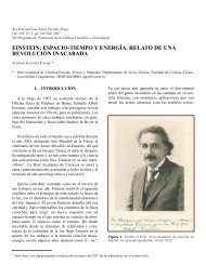
D. CHICO et al. 21FIGURE 3. Average green, blue and grey water footprint of Spanishtomato (l/kg)Source: Own elaboration.There are important differences in the volume, type, andpurpose of the production between the different productionprovinces which derive in different water footprint of tomato.Figure 5 summarizes the average green, blue and greywater footprint (l/kg) in all the Spanish provinces in decreasingorder.As shown, the water footprint varies significantly betweenthe different provinces, and so does the proportion ofthe green, blue and grey components. These differences maybe due to the predominant production system (open-airrainfed or irrigated vs. covered) in the province, yields obtainedand climate parameters (precipitation and atmosphericevapotraspiration demand). In general, we can seethat the grey water footprint is the main source of variability,whereas the green water footprint is in general termsrather low.

22 THE WATER FOOTPRINT OF TOMATO PRODUCTIONFIGURE 4. National green, blue and grey water footprint (WF) (hm 3 , leftaxis), average yield (t/ha), national tomato production (1,000,000 t) andweighed water use (1,000 m 3 /ha) (right axis)Source: Own elaboration.As illustrated in figure 5 most of the main producingprovinces have a total water footprint below the nationalaverage. This may be related to the high yields achieved inthese provinces. In Figure 6 the total water footprints inhm 3 of the main producing provinces are represented, alongwith the average annual water footprint of all the provincesas a reference point and the percentage of national productioneach province represents.Again, we observe that the relative differences betweenthe green, blue and grey water footprints are maintained,being the grey water footprint the most important component.The high production of Badajoz and Almería makes

D. CHICO et al. 23FIGURE 5. Average green, blue and grey water footprint (WF) (l/kg) inthe different Spanish provinces (l/kg, left axis) and annual production(t, right axis)Source: Own elaboration.

24 THE WATER FOOTPRINT OF TOMATO PRODUCTIONFIGURE 6. Annual green, blue and grey water footprint (hm 3 ) of Spanishtomatoes for the main producing provinces and average percentage ofnational productionSource: Own elaboration.the total water footprint soar, although both provinces haverelatively small water footprints in terms of l /kg and highefficiencies (Figure 5). In the province of Almería most ofthe water bodies are at risk of no compliance with the EuropeanWater Framework Directive (Andalusian WaterAgency, 2010), as so are in Badajoz the groundwater bodiesand the Guadiana river itself (CHG, 2009).3.2. Disaggregated water footprint: Analysisbetween production systemsThe main components of the water footprint are very dependenton the production system and actually vary signif-

D. CHICO et al. 25FIGURE 7. Average green, blue and grey water footprint (WF) of openair (rainfed and irrigated) and greenhouse production (l/kg)Source: Own elaboration.icantly even within the same province. Moreover, tomatoand in general horticultural crops may be grown within awide range of production systems in mild climates. In theSpanish case, this whole range is covered, with production(albeit small) of rainfed tomato, low intensity traditionaltomato, highly productive intensive open-air tomato and themost intensive, even technology-driven greenhouse production(Maroto, 2002; Nuez, 1995).As already mentioned, there are sharp differences in thewater footprint across production systems. Rainfed tomatoproduction has by far the highest water footprint with 966l/kg. The grey water footprints of open-air irrigated andgreenhouse production systems are small in comparison toit, partly due to their much higher yields. The Nitrogen bal-

26 THE WATER FOOTPRINT OF TOMATO PRODUCTIONFIGURE 8. Yearly average green, blue and grey water footprint (WF)per production system of the main producing provinces (hm 3 )Source: Own elaboration.ance data used for the calculation of the grey water footprintdid not distinguish between the different productionsystems, being the resulting grey water footprints thereforeinversely proportional to the yield. It must be noted thatthese results are given in terms of l/kg.When analysing the water footprint in terms of total cubicmeters, the tomato water footprint is very concentrated ina few productive areas. Figure 8 represents the green, blueand grey water footprint of the eight most productive Spanishprovinces per production system and their average annualwater footprint. In accordance with Figure 6, Badajozand Almería are the two provinces with the highest totalwater footprint (hm 3 ).

D. CHICO et al. 27TABLE 3. Percentage of green, blue and grey water footprint per production system of the mostproductive provinces (1,000 m 3 )ProvinceAv. Green Av. Grey Av. Green Av. Blue Av. Grey Av. Blue Av. Grey Totalwater water water footprint water footprint water footprint water water Waterfootprint footprint Open-air Open-air Open-air footprint footprint FootprintRainfed Rainfed irrigated irrigated irrigated Greenhouse Greenhouse (hm 3 )Badajoz 3 51 46 215Almería 0.3 4 12 30 54 183Murcia 1 11 26 20 42 80Las Palmas 0.1 0.5 0 6 10 35 48 26Granada 1 9 39 15 37 42Cáceres 2 51 47 45Sevilla 0.2 1 2 64 32 0.1 1 25Navarra 3 28 68 0.5 1 44

28 THE WATER FOOTPRINT OF TOMATO PRODUCTIONIn all cases the green water footprint is practically negligible.It should also be noticed that the grey water footprintof both Badajoz and Almería is similar, even if theproduction is greater in Badajoz. This is related to the higherexcess of Nitrogen in Almería, 139 kg N/ha as comparedto 68 kg/ha of Badajoz (MARM, 2008) (Appendix IV).However, different green, blue and grey water footprintproportions are found across production regions. In this regard,we see that the main component of the water footprintin Badajoz is the blue one (of the open-air irrigated production)whereas in Almería it is the grey one. Something similarhappens in the rest of the provinces.If the water footprint is an indicator of the water appropriationof a product (Hoekstra et al., 2009), its compositionmay help us identify the main areas of impact of its production.The main primary impact of the tomato productionin Badajoz, (also in Cáceres or Sevilla) would be the highvolume of blue water consumed, whereas in Almería (andMurcia, Navarra or Granada) would be the pollution of waterresources. It is through this type of analysis where thewater footprint reveals itself as a powerful indicator.4. APPARENT WATER PRODUCTIVITY AND VIRTUAL WATEREXPORTS OF TOMATO PRODUCTION4.1. Water apparent productivity of tomatoproductionThe apparent water productivity (WAP) is an indicator ofthe economic performance of the water use. As shown in Tables4 and 5 the water apparent productivity of tomato productionvaried from 0.025 to 36 €/m 3 , depending on the productionsystem, type of water (green or blue) and on the

D. CHICO et al. 29TABLE 4. Proportion of green and blue water footprint (WF) in open-airirrigated systems and average apparent water productivity (WAP) of themain producing provinces under different production systems (€/m 3 )Proportion of WF Proportion WAP of WAP of open-air WAP ofProv. Green WF vs. of Blue WF rainfed irrigaton greenhousesTotal WF vs. Total WF systems (€/m 3 ) systems (€/m 3 ) (€/m 3 )Badajoz 5.9 94.1 3.1 0.03Almería 6.0 94.0 3.9 7.1Murcia 6.8 93.2 3.8 3.9 8.8Las Palmas 4.2 95.8 18.1 4.6 9.3Granada 9.0 91.0 7.3 7.2Cáceres 4.7 95.3 2.2Sevilla 3.1 96.9 2.6 3.1 127.4Navarra 7.4 92.6 3.4 6.3National average 8.7 91.6 2.1 3.1 7.8season of the year. On average, the WAP of tomato was about5 €/m 3 . In the tomato production, the prices vary significantlydepending on the time of the year, being a stimulus for offseasonproductions (autumn and winter) where it is possible.Tables 4 and Table 5 show the apparent productivity of waterover the different production periods of the year and productionsystems for the main producing provinces.As shown in table 4, greenhouse production has muchhigher productivity compared to open air, irrigated. The relativelylow productivity of rainfed production leads to ahigher water footprint of this production system. As shownin Table 5 the productivity of tomatoes in the early and lateseason is much higher than that of the middle season. Inthe Spanish case, these productions correspond mainly togreenhouse production.However, some of the values obtained seemed to be toohigh to be realistic (e.g. apparent water productivity of Sevillaprovince under greenhouses). Apparent water productivityis calculated at market price and in correspondence with

30 THE WATER FOOTPRINT OF TOMATO PRODUCTIONTABLE 5. Proportion of green and blue water footprint (WF) and average apparent water productivity of themain producing provinces in relation to the year season (€/m 3 )Prop. of Prop. of Prop. of Prop. of Prop. of Prop. ofGreen Blue WF WAP Green WF Blue WF WAP Green WF Blue WFProvinceWF vs. vs. Total ( €/m 3 ) vs. Total vs.( €/m 3 ) vs. Total vs. TotalTotal WF WFWF Total WFWF WFWAP( €/m 3 )Badajoz 3 97 5.7 5 95 3.8 2 98 10.4Almería 6 94 9.3 22 78 2.1 3 97 7.9Murcia 28 72 9.2 24 76 3.4 24 76 10.4Las Palmas 5 95 11.8 5 95 3.8 3 97 11.1Granada 5 95 2.2Cáceres 1 99 22.7 39 61 3.0 1 99 24Sevilla 5 95 3.3 6 94 4.7Navarra 20 80 7.5 24 76 2.7 15 85 9.5Nationalaverage3 97 5.7 5 95 3.8 2 98 10.4

D. CHICO et al. 31the water footprint. In these cases, the small share of a particularproduction system and/or season of the provincialproduction is probably a source of bias. For example, in thecase of Sevilla province, the average area under greenhouseis 33 ha compared to 2196 ha of tomato production or 13 haof rainfed tomato in Las Palmas province compared to 2031ha cultivated annually for tomato production. These smallsurfaces, together with recorded yields, as shown in the statisticaldatabases should probably be reviewed.4.2. Water apparent productivity of surfaceor groundwaterIn this section, the water apparent productivity is analyseddepending on the origin of water; ground or surface water.Information on the origin of irrigation water specifically forhorticultural production in each province is not directly available.However, in some of the main productions provinces,the water is overwhelmingly of a specific origin; surface inthe case of Badajoz, Cáceres and Navarra provinces (CHG,2008) and groundwater in the case of Almería (Regional Governmentof Andalusia 2003) and Canary Islands (Las Palmasand Tenerife provinces). These six provinces represent 61%of the yearly national production.The origin of the water is related to the production system.In these cases, the provinces using surface water producearound 98% of their production in open-air systems while thetwo provinces accounted for with groundwater produce over90% of their tomatoes in greenhouses. As seen in Table 4 thegroundwater apparent productivity is notably higher than surfacewater productivity. It clearly exceeds the average productivityof blue water used in irrigated agriculture in Spain,which is about 0.44 €/m 3 according to the Spanish Ministry ofthe Environment and Rural and Marine Affairs (MARM, 2007).

32 THE WATER FOOTPRINT OF TOMATO PRODUCTIONTABLE 6. Water apparent productivity of surface and groundwater irrigation (€/m 3 )Open-airirrigated WAP(€/m 3 )Greenhouse Early season Middle season Late season Av. WAPWAP (€/m 3 ) WAP (€/m 3 ) WAP (€/m 3 ) WAP (€/m 3 ) €/m 3 )Surface 3.0 6.4 2.8 4.7 3.0Groundwater 4.1 7.6 6.5 3.7 10.5 7.2

D. CHICO et al. 334.3. Virtual water exportsAs explained above, the production of tomatoes in Spainis to a high degree intended for export, especially in thesoutheastern Mediterranean provinces. In this case, theproduction is highly dependent on international marketsand competition from other areas (García Martínez, 2009;Colino, 2002).As an average of the study period, the yearly amount ofvirtual water exported through the tomato exports is 4, 88and 134 hm 3 of green, blue and grey water respectively. Spanishtomato exports are to a very high degree directed towardsFIGURE 9. Virtual water exports (hm 3 , left axis), exported tonnes of freshtomatoes to the world and to the EU, apparent water productivity of theexported production (€/m 3 , right axis) and revenues of the tomatoexports (1,000 €, right axis)Source: Own elaboration.

34 THE WATER FOOTPRINT OF TOMATO PRODUCTIONthe European Union, being the UK, Germany and the Netherlandsthe main importers (MITYC, 2009). As an average, 93%of the virtual water exports correspond to the EU.The average water apparent productivity of the exportedproduction in the period was 8.8 €/m 3 . This productivity ishigher than the average WAP of 5 €/m 3 , and closer to 7.1€/m 3 of greenhouse production and to 7.2 €/m 3 correspondingto production using groundwater. These results are actuallyclosely related, since the main exporting provinces, Almería,Murcia and Las Palmas, have a production mainly undergreenhouses conditions, using groundwater and in early andlate season (MARM, 2010b; Suárez, 2002 García, 2009). Togetherthey represent more than 60% of the annual exports(MICYT, 2009).5. DISCUSSIONThis study provides a detailed analysis of the green, blueand grey water footprint of tomato production in Spain, bothin l/kg and hm 3 , for all the Spanish provinces during theperiod 1997-2008.The results obtained for the average green and blue waterfootprint in terms of l/kg were in the range of those fromother studies, whereas the values obtained for the averagegrey water footprint were much higher. For tomato productionin Spain, Chapagain and Orr (2009) obtained values ofabout 14, 60 and 7 l/kg for the green, blue and grey waterfootprint respectively. In their study of the water footprintof tomato production in Italy, Aldaya et al. (2010) calculatedvalues of 35, 60 and 19 l/kg for green, blue and grey waterfootprint respectively. These differences with the study ofChapagain and Orr may be related to the different datasources and assumptions made. We followed the Nitrogen

D. CHICO et al. 35Balance of the Spanish Ministry of the Environment andRural and Marine Affairs, which presents rather high valuesfor excess Nitrogen (MARM, 2008), 112 kgN/ha as a nationalaverage. In the case of Chapagain and Orr, they consideredthe leaching Nitrogen to be 25kg/ha from open and15 kg/ha from covered systems following Mema et al. (2005).As for the study of Aldaya et al. used an estimated leachingof 10 % of the estimated applied rate of 110 kg/ha fromFertistat database (FAO, 2010).The main producing provinces (Badajoz, Almería and ina lesser extent Murcia, Las Palmas, Granada, Sevilla,Cáceres and Navarra) are among the most effective in termsof l/kg, having achieved large yields and productivitiesthanks to intensification (García, 2009; Suárez, 2002). However,due to their huge cumulative total productions theirwater footprints are also significantly higher than the rest.This shows the pressure on the water resources in theseprovinces. For instance, in Almeria most of the aquifers inthe province are at risk of non-compliance with the objectivesby the EU Water Framework Directive (AndalusianWater Agency, 2010), so are in Badajoz the groundwaterbodies and the Guadiana river itself (CHG, 2009). As expectedfor a horticultural crop, the green water footprint isalmost negligible, both for rainfed and for irrigated openairproduction. An interesting analysis would be the studyof the social revenues of this pressure.As explained above, one of the reasons for the differentwater footprint results from other studies may be relatedto the different data used and assumptions taken to modelthe crop water use. A change in, for example, the length ofthe growing period may notably vary the crop water useand thereafter the green and blue water footprint obtained.Despite this, the values obtained here were in the samescale as those from other authors for the green and blue

36 THE WATER FOOTPRINT OF TOMATO PRODUCTIONwater footprint of tomatoes in Spain (Chapagain and Orr,2009; Madrid and Velázquez, 2008; Aldaya and Llamas,2009). Chapagain and Orr (2009) obtained an average greenand blue water footprint of 74 m 3 /t, compared to our 92 m 3 /t.Madrid and Velázquez (2008) studied the Andalusia region,obtaining blue water values of 80 m 3 /t, which in our casewas 58 m 3 /t as an average for this region. Aldaya and Llamas(2009), in their study of the Guadiana river basin calculated6 and 115 m 3 /t for the green and blue water footprintin open air irrigated tomato of the middle Guadianabasin, which corresponds to Badajoz province. In our case,the average water footprint for this production system wasvery similar; amounting to 6 and 103 m 3 /t. Garrido et al.(2010) calculated an average green and blue water footprintof tomato production of 95 m 3 /t.The estimation of leached Nitrogen is a very context specificfactor. With this in mind, we tried to make an approximation,based on the Nitrogen balances. The values obtainedshould be taken as a first approximation, by nomeans we consider it a definitive measurement. With thismethodology, we made a number of assumptions in orderto calculate the grey water footprint. First, the excess Nitrogenfrom the N balance data of the Spanish Ministry ofthe Environment and Rural and Marine Affairs are providedfor the year 2006 (MARM, 2008). Excess Nitrogen thereforewas assumed to be constant throughout the years foreach province and between production systems. The resultinggrey water footprint thus mainly depends on the yieldsused. Besides, the excess Nitrogen data does not distinguishbetween rainfed and irrigated farming. Since the rainfedproduction has a very limited area, its weight in the Nitrogenbalance calculation is limited and may not be representative.Secondly, no temporal calculation less than a yearwas taken into account. Lixiviation occurs on early stagesof the crop and is sharply dependent on precipitation

D. CHICO et al. 37(Vázquez et al., 2003). In their study of the N lixiviationfrom open air, drip irrigated tomatoes in Ebro valley,Vazquez et al. (2003) measured leaching N values of 155-421 kg N /ha, which were very dependent on the irrigationschedule, available N at the beginning of the season andprecipitation. The value taken here for La Rioja was 161 kgN /ha. Within our scope, it was impossible to account forsite- and management- specific factors, so further refinementsare clearly necessary.As for the case of the Almería province (and this can probablybe generalized to production in greenhouses in southeastSpain), the N pollution may also be a consequence oflarge irrigation prior to transplanting and during the first6 weeks of the crop. This irrigation, combined with largemanure applications (as part of the artificial soils) and generousfertilizations may lead to high Nitrogen lixiviation(Thompson, 2007). In our case, this was indirectly reflectedthrough the N balance data of the Spanish Ministry of theEnvironment and Rural and Marine Affairs, with values ofabout 139 N/ha. This balance however may be underestimatingthe amount of N available for leaching. Thompsonet al. (2002) observed a mean value of 527 kg N /ha at 60cm depth in greenhouses in Almería. They mentioned thevariability of the data, reassuring the difficulty of makingaccurate estimations.Another limiting factor of our study is that many of themain producing provinces developed and changed significantlytheir irrigation techniques during the study period.Irrigation technologies, schemes and applications haveevolved since 1997. So have the growing technologies, suchas plastic mulch in open-air production (Campillo, 2007;Macua and Lahoz, 2005), or greenhouses’ technologicalchange (García, 2009; Céspedes, 2009), which could haveled to different soil moisture balances and thereafter to dif-

38 THE WATER FOOTPRINT OF TOMATO PRODUCTIONferent crop water uses. This factor was not taken into account,so the analysis of the temporal evolution of theprovinces could be improved. In any case, the scope of thisstudy is different as we intended to cover the whole countryand for a relatively long period.The apparent water productivity (€/m 3 ) varied significantlynot only between production systems, but also betweenperiods of the year. The productivities were significantlyhigher for greenhouse production and for early andlate season productions. These results are related since productionin early (January to May) and late (October to December)seasons are done mainly in greenhouses, whichcompensates the adverse climatic conditions of these periods.Along with this, these productions are to a high degreeintended for export markets and consumed in other countries(García, 2009) and therefore focus on a high-qualityvaluable product (Castilla, 2007). This way, Spanish waterresources are virtually exported away from the country inexchange for revenues.The differences in the apparent water productivity wouldprobably have been sharpened if we had distinguished theprices of the tomatoes for provinces and growing systems,specially separating production for fresh consumption fromproduction for the industry as the price of both products isvery different. Still, this is reflected to a certain degree inour work. In general terms, the production areas (and theprovinces) “specialise” themselves in specific productions foragronomical and socio-economical reasons.The analysis of the apparent water productivity in relationto the origin of water did show clearly that groundwateris more productive than surface one. This is alsoreflected in the type of production in which each of themis used. Surface water is predominantly used in areas

D. CHICO et al. 39where the main production system is open-air irrigation.In many cases (though not exclusively) this type of productionis intended for processing tomato, as in the MiddleGuadiana and Ebro Valleys, which has a lower marketprice. Groundwater is generally used in areas where theproduction is intended for export and has higher prices.These results confirm previous studies that claim thatagriculture using groundwater is economically more productivethat using surface water (Hernández-Mora et al.,2001; Llamas and Martínez-Santos, 2005). This differencecan be attributed to several causes: the greater controland supply guarantee that groundwater provides, whichin turn allows farmers to introduce more efficient irrigationtechniques and more profitable crops; the greater dynamismthat has characterized the farmer that hassought out his own sources of water and bears the fullcosts of drilling, pumping and distribution; and the factthat the higher financial costs farmers bear motivatesthem to look for more profitable crops that will allow themto maximize their return on investments (Hernández-Mora et al., 2001).Finally, as for the water footprint of tomato exports, theywere assigned to each province proportionally to their shareof the national production. The international trade database(DataComex) of the Spanish Ministry of Industry,Tourism and Commerce reflects where the amount of tomatoesleft the country, not where they were produced. Hadwe applied the water footprint of the exporting province tothe tomatoes exported, it would have meant an overestimationof the water footprint of the exports of the provinceswith intensive international commerce while ignoring thoseproducing the tomatoes. In any case, a more detailed analysisof the export character of particular provinces would beadvisable to better quantify the water footprint other nationshave in Spain.

40 THE WATER FOOTPRINT OF TOMATO PRODUCTION6. CONCLUSIONThe total water footprint of 1 kilogram of tomato producedin Spain is about 236 litres per kilogram, ranging from 216to 301 litres per kilogram. The colours of the total averagewater footprint are as follows: 3% green, 36% blue and 58%grey. Still, these averages vary greatly depending on thecrop and water management systems, location and climate.Total largest footprints (hm 3 ) correspond, logically, to thetwo main producing provinces; Badajoz and Almería. Theyare well ahead of the rest of the provinces with an averageof 215 and 182 hm 3 per year. In contrast, these twoprovinces show a high efficiency in terms of water use (l/kg),standing below the national average of 235 l/kg, with 201l/kg for Badajoz and 228 l/kg for Almería.The large differences of water footprints across provinces,years and production systems, indicate the relevance of evaluationscarried out at the lowest possible scale. The nationalannual average water footprint in terms of l/kg for rainfed,open-air irrigated and greenhouse production systems was73, 331 and 74 l/kg respectively. Greenhouse production obtainsvery high yields that compensate their water use.The average water apparent productivity of tomato productionwas about 2, 3 and 8 €/m 3 for rainfed, open-air irrigatedand greenhouse production systems respectively.We note also the important differences in the apparent waterproductivity throughout the year, which may be relatedto the much higher price of off-season productions.Groundwater production presented a higher blue water apparentproductivity than that of open-air irrigated production,around 7 €/m 3 compared to 3 €/m 3 . In any case, the studyin this field included only some provinces with specific and

D. CHICO et al. 41different productions. While the provinces irrigated with surfacewater produce mainly tomatoes intended for the industryin open-air systems, those accounted for as irrigated withgroundwater produce fresh tomato for export, more valuable.Virtual water exports related to tomato exports representabout 2.5% of total Spanish water exports, without consideringgrey water (Garrido et al., 2010). However, in economicterms (€/m 3 ) tomato exports are 350% larger than the averageexports (Garrido et al., 2010), with 8.81 €/m 3 comparedwith the average 2.5 €/m 3 of the average exports. Reducingthe blue and green water footprint of tomato production willnot be easy because of plant physiology restrictions, but thegrey water component can be significantly reduced. Shouldthis be achieved by optimizing the timing and technique ofNitrogen applications, so that less is needed and/or lessleaches or runs off, Spanish tomato exports’s sustainabilitywould significantly improve. Water footprint evaluationsthat omit the grey component would lead to incomplete conclusions,as they may lead to increase efficiency in direct waterconsumption but fail to take into account the environmentalpressure related to pollution.Finally, the water footprint contextualized in space andtime can provide useful information for benchmarking, indentifyingbest practices and achieving a more integratedwater resource management. However, to obtain a comprehensivepicture, not only the (eco) efficiency in terms ofm 3 /ton should be considered, but also the context-specific totalcumulative water footprint.7. ACKNOWLEDGEMENTSWe would like to thank Professor A. Saa, J. M.ª Duránand C. Hernández of the Technical University of Madrid for

42 THE WATER FOOTPRINT OF TOMATO PRODUCTIONtheir help and useful advices. We also would like to thankthe M. Botín Foundation for financially supporting thisproject. The contents of the report remain the responsibilityof the authors.9. REFERENCESAldaya, M. M. and Llamas, M.R. (2009) Water Footprint Analysis (Hydrologicand Economic) of the Guadiana River basin. The United NationsWorld Water Assessment Programme, Scientific Paper. United NationsEducational, Scientific and Cultural Organization, ParisAldaya, M. M. and Hoekstra, A. Y., (2010) The water needed for Italiansto eat pasta and pizza. Agricultural systems 103, 351-360.Andalusian Water Agency (2010). Proyecto del plan hidrológico de la demarcaciónhidrográfica de las cuencas mediterráneas andaluzas. [online]Available from:http://www.juntadeandalucia.es/medioambiente/site/web/menuitem.a5664a214f73c3df81d8899661525ea0/?vgnextoid=c00b8e2d2f5b8210Vgn-VCM1000001325e50aRCRD&vgnextchannel=ee8feb3d87605210Vgn-VCM1000001325e50aRCRD [accessed on July 2010].Bertuglia, A. and Calatrava Requena, J. (2008) Las explotaciones hortícolasbajo plástico del litoral oriental granadino. Horticultura internacional, 64.Campillo, C. (2007) Estudio para el diseño de un sistema de recomendaciónde manejo de agua en rotaciones de cultivo hortícolas en las vegas del Guadiana.Tesis Doctoral, Universidad de Extremadura.Castilla, N. (2007) Invernaderos de plástico: Tecnología y manejo. 2ª ed.,Ed. Mundi-Prensa, Madrid, Spain.CEC, M.Th., 1985. Soil Map of the European Communities Office for OfficialPublications for the EC, Luxembourg. 124 pp. 7 maps.

D. CHICO et al. 43Céspedes López, A.J. García García, M.C. Pérez Parra, J.J. and CuadradoGómez, I.M. (2009) Caracterización de la explotación hortícola protegidaalmeriense. Ed. F.I.A.P.A. y fundación CajaMar.Chapagain, A. K. and Hoekstra, A. Y. (2004) Globalization of water. Sharingthe planet’s freshwater resources. Ed. Blackwell Publishing, Oxford, UK.Chapagain, A. K. and Orr, S. (2009) An improved water footprint methodologylinking global consumption to local water resources: A case of Spanishtomatoes, Journal of Environmental Management, 90.Colino Sueiras, J. and Martínez Paz, J. M. (2002) El agua en la agriculturadel sureste español: Productividad, precio y demanda; in La agriculturamediterránea en el siglo XXI. Coord.: García Álvarez-Coque, J. M. ColecciónMediterráneo económico, nº2. Ed: Caja Rural Intermediterránea. Cajamar.Comisión Europea (2002) Aplicación de la Directiva 91/676/CEE del Consejorelativa a la protección de las aguas contra la contaminación producidapor nitratos utilizados en la agricultura. Síntesis de los informes de losEstados miembros del año 2000. Comisión Europea, Dirección General deMedio Ambiente. [online] Available from: http://europa.eu.int. [Accessed onJune 2010]CHG, Confederación hidrográfica del Guadiana (2009) Borrador del planhidrológico de la Demarcación hidrográfica del Guadiana. Estudio generalde la demarcación hidrográfica del Guadiana. Parte II. . [online] Availablefrom: http://planhidrologico2009.chguadiana.es/corps/planhidrologi-co2009/data/resources/file/documentos/DOCaconsulta/primeraetapa/RE-SUMENCARACTERIZACIONPARTEII.pdf[Accessed on September 2010].Falkenmark, M. (2003) Freshwater as shared between society and ecosystems:from divided approaches to integrated challenges. PhilosophicalTransactions of the Royal Society B: Biological Sciences, 358 (1440): 2037–2049.

44 THE WATER FOOTPRINT OF TOMATO PRODUCTIONFalkenmark, M. and Rockström, J. (2004) Balancing water for humansand nature: The new approach in ecohydrology, Earthscan, London, UK.FAO (1998) Allen, R.G., Pereira, L.S., Raes, D. and Smith, M. Crop evapotranspiration- Guidelines for computing crop water requirements - FAOIrrigation and drainage paper 56. Food and Agriculture Organization.Rome.FAO (2009) CROPWAT 8.0 model, Food and Agriculture Organization,Rome, Italy. [online] www.fao.org/nr/water/infores_databases_cropwat.html.[Accessed on January 2001].FAO-UN (2007) Digital Soil Map of the World. [online] Available from:http://www.fao.org/geonetwork/srv/en/main.home [Accessed on June 2010]Fernández M.ª D., Orgaz, F. Fereres, E. López, J. C. Céspedes, A. Pérez,J. Bonachela, S. and Gallardo, M. (2001) Programación del riego de cultivoshortícolas bajo invernadero en el sudeste español. Ed. CajaMar. Almería,Spain.García Martínez, Mª. C. (2009) La adopción de tecnología en los invernaderosmediterráneos. Tesis doctoral , Universidad politécnica de Valencia.Garrido A., Llamas, R. Varela-Ortega, C Novo, P. Rodríguez-Casado, R.and Aldaya, M. M. (2010) Water footprint and virtual water trade in Spain.Policy implications Ed. Springer New york.Gil de Carrasco, C. Miras, R, Boluda Hernández, R. and Picazo Vico, P.(2001) Caracterización físico-química y evaluación del estado de los suelosen los invernaderos del poniente almeriense F.I.A.P.A. publicaciones. Boletínn.º 13.Hernández-Mora N., Llamas M.R. and Martínez-Cortina L. (2001) Misconceptionsin aquifer over-exploitation. Implications for water policy in SouthernEurope. Agricultural Use of Groundwater: Towards Integration be-

D. CHICO et al. 45tween Agricultural Policy and Water Resources Management, Dosi C. (ed.).Dordrecht, The Netherlands, Kluwer Academic Publishers, pp.107–25.Hoekstra, A.Y. (ed.) (2003) Virtual water trade: Proceedings of the InternationalExpert Meeting on Virtual Water Trade, Delft, The Netherlands,12–13 December 2002, Value of Water Research Report Series No.12, UN-ESCO-IHE, Delft, the Netherlands.Hoekstra, A.Y. and Chapagain, A.K. (2008) Globalization of water: Sharingthe planet’s freshwater resources. Blackwell Publishing. Oxford, UK.Hoekstra, A.Y., Chapagain, A.K., Aldaya, M.M. and Mekonnen, M.M.(2009) Water footprint manual: State of the art 2009, Water Footprint Network,Enschede, the Netherlands.Hoyos, P. (2005) El cultivo del tomate para fresco: situación actual y perspectivasdesde el punto de vista técnico y comercial. Ed. MARM, San Fernandode Henares, Spain.Llamas, M.R. and Martínez-Santos, P. (2005) Intensive groundwater use:silent revolution and potential source of social conflicts, Journal of WaterResources Planning and Management. Vancouver, USA American Societyof Civil Engineers (ASCII), pp. 337–41.Macua J.I. and Lahoz I. (2005) Evolución del tomate de industria en Navarraen los 25 años del Itg Agrícola. Navarra agraria, 153.Madrid, C. and Velázquez, E. (2008) El metabolismo hídrico y los flujos deagua virtual. Una aplicación al sector hortofrutícola de Andalucía (España)Revista de la red iberoamericana de economía ecológica, vol 8.MARM (2002) Calendario de siembra y recolección (años 1996-1998). SpanishMinistry of the Environment and Rural and Marine Affair of Spain.Ed. Secretaría General de Medio Rural. Madrid, Spain.MARM (2007) El agua en la economía española: Situación y perspectivas.Spanish Ministry of the Environment and Rural and Marine Affairs.

46 THE WATER FOOTPRINT OF TOMATO PRODUCTIONMARM (2008) Nitrogen balance of the spanish agriculture (año 2006).Spanish Ministry of the Environment and Rural and Marine Affairs. [online]Available from: http://www.ruena.csic.es/balances.html [Accessed onJuly 2010].MAPA (2010a) Sistema de Información Agroclimática para el Regadío(SIAR). Spanish Ministry of the Environment, and Rural and Marine Affairs.[online] Available from:http://www.mapa.es/siar/Informacion.asp [Accesed on Juny 2010]MARM (2010b) Agricultural and Statistics Yearbooks. Spanish Ministryof the Environment, and Rural and Marine Affairs. [online] Available from:http://www.mapa.es/es/estadistica/pags/anuario/introduccion.htm [Accessedon July 2010]MARM (2010c) cover of irrigated areas, WMS of the Spanish Ministry ofEnvironment, and Rural and Marine Affairs. [online] Available from:http://wms.Marm.es/sig/Regadios/wms.aspx [Accessed on May 2010]Maroto, J. V. (2002) Horticultura herbácea especial. Ed. Mundi-Prensa 5ªed. Madrid, Spain.Mema, M. Calvo, E. Albiac, J. (2005) Agricultural nonpoint pollution inAragón: Emmission loads and concontrol issues,. Agrifood Research andTechnology Centre, University of Zaragoza, Spain. : in Chapagain, A. K.and Orr, S. (2009) An improved water footprint methodology linking globalconsumption to local water resources: A case of Spanish tomatoes, Journalof Environmental Management, 90.MITYC (2009) Datacomex, Estadísticas de comercio exterior. Spanish Ministryof Industry, Tourism and Commerce. [online] Available from:http://datacomex.comercio.es/ [accessed on July 2010]Nuez, F. (1995) El cultivo del tomate. 3ª ed., Ed. Mundi-Prensa, Madrid,Spain.

D. CHICO et al. 47Orgaz, F. Fernández, M. D. Bonachela, S. Gallardo, M. Fereres, E. (2005)Evapotraspiration of horticultural crops in an unheated plastic greenhouse.Agricultural water management, 72.Reche Mármol, J. (2009) cultivo del tomate en invernadero. Ed. M.AR.M.Madrid, Spain.Regional Government of Andalusia (2003) Inventario y caracterización delos regadíos de Andalucía:actualización 2002 [Software: 18 files and 33 megabytes].Servicio de Regadíos e Infraestructuras, Junta de Andalucía. Cádiz: Servicio de Publicaciones y Divulgación.Smakhtin, V., Revenga, C., and Döll, P. (2004a) Taking into account environmentalwater requirements in global-scale water resources assessments,Comprehensive Assessment Research Report 2, IWMI, Colombo,Sri Lanka.Suárez Bosa, M. and Ojeda Déniz, P. (2002) Evolución del cultivo del tomateen Canarias desde la incorporación a la Unión Europea (1986-2001).Estudios agrosociales y pesqueros, n.º 196.Thompson, R. B. C. Gallardo, and M. Giménez, (2002) Assesing risk of Nitrogenleaching from the horticultural industry of Almería, Spain. Workshoptowards an ecologically sound fertilization in field vegetable production.Proceedings. Ed. Booij, R. Neeteson, J. Wageeningen, TheNetherlands.Thompson, R. B. Martínez-Gaitan, O. C. Gallardo, M. Giménez, C. andFernández, M. D. (2007) Identification of irrigation and N managementpractices that contribute to nitrate leaching loss from an intensive vegetableproduction system by use of a comrehensive survey. Agriculturalwater management, 89.UNESCO (2006) Water, a shared responsibility: The United Nations worldwater development report 2. UNESCO Publishing, Paris / BerghahnBooks, Oxford.

48 THE WATER FOOTPRINT OF TOMATO PRODUCTIONVázques, N. Pardo, A. Suso, M.ª L. and Quemada, M. (2003) Drenaje y lixiviadode nitratos en una sección transversal de un sistema de cultivohortícola con riego por goteo y acolchado plástico. Revista de Estudio dela Zona No Saturada del Suelo, vol VI.

D. CHICO et al. 4910. APPENDIXAPPENDIX I. Planting and harvesting dates for each season and type of soil in relation to tomato productionin the different Spanish provincesProvincesEarly season Middle season Late seasonSoiltexture Planting Harvesting Planting Harvesting Planting Harvestingdate date date date date dateLa Coruña Loam May-01 Sep-01 Jun-01 Oct-01Álava Loam Apr-01 Aug-01 May-01 Oct-01Albacete Clay-Loam May-01 Sep-01Alicante Loam Dec-01 Apr-01 Apr-01 Aug-01 Jul-01 Dec-01Almería Clay-Loam Jan-01 Apr-01 Jan-01 Jun-01 Aug-01 Dec -01Asturias Loam May-01 Sep-01 Jun-01 Oct-01Ávila Clay-Loam May-01 Aug-01 Jun-01Badajoz Loam Mar-01 Aug-01Baleares Clay-Loam Dec-01 May-01 Apr-01 Aug-01 May-01 Oct-01Barcelona Loam Apr-01 Aug-01 Apr-01 Oct-01Burgos Loam May-01 Aug-01 Jun-01Cáceres Loam May-01 Sep-01Cádiz Loam Nov-01 Mar-01 Mar-01 Aug-01 Aug-01 Nov-01Cantabria Loam May-01 Sep-01 Jun-01 Oct-01Castellón Loam Jan-01 May-01 Mar-01 Jul-01 Jul-01 Oct-01Ciudad Real Clay-Loam May-01 Sep-01 May-01 Sep-01Córdoba Loam Apr-01 Aug-01Cuenca Loam Jan-01 Aug-01

50 THE WATER FOOTPRINT OF TOMATO PRODUCTIONAPPENDIX I. Planting and harvesting dates for each season and type of soil in relation to tomato productionin the different Spanish provinces. (Cont.)ProvincesEarly season Middle season Late seasonSoiltexture Planting Harvesting Planting Harvesting Planting Harvestingdate date date date date dateGirona Loam Apr-01 Aug-01 Jun-01 Oct-01Granada Clay-Loam Dec-01 Apr-01 Mar-01 Jul-01 Aug-01 Dec-01Guadalajara Clay May-01 Sep-01Guipúzcua Loam Apr-01 Aug-01 May-01 Oct-01Huelva Clay-Loam Dec-01 Apr-01 Apr-01 Aug-01 Jul-01 Nov-01Huesca Clay Apr-01 Sep-01 May-01 Oct-01Jaén Loam May-01 Aug-01 Aug-01 Nov-01La Rioja Loam May-01 Sep-01 May-01 Oct-01Las Palmas Loam Oct-01 Feb-01 Apr-01 Jul-01 Aug-01 Dec-01León Loam Jun-01 Sep-01Lérida Loam Feb-01 Aug-01 Jun-01 Oct-01Lugo Loam May-01 Sep-01 Jun-01 Oct-01Madrid Loam Apr-01 Jul-01Málaga Loam Dec-01 Apr-01 Mar-01 Jul-01 Jul-01 Dec-01Murcia Clay-Loam Oct-01 Mar-01 Apr-01 Aug-01 Jul-01 Nov-01Navarra Loam Apr-01 Sep-01 May-01 Oct-01Orense Loam May-01 Sep-01 Jun-01 Oct-01Palencia Loam May-01 Aug-01Pontevedra Loam May-01 Sep-01 Jun-01 Oct-01Salamanca Loam Jun-01 Sep-01Segovia Clay-Loam May-01 Sep-01

D. CHICO et al. 51APPENDIX I. Planting and harvesting dates for each season and type of soil in relation to tomato productionin the different Spanish provinces. (Cont.)ProvincesEarly season Middle season Late seasonSoiltexture Planting Harvesting Planting Harvesting Planting Harvestingdate date date date date dateSevilla Loam Mar-01 Jun-13 Apr-01 Aug-01 Aug-01 Nov-01Soria Loam May-01 Aug-01Tarragona Loam Feb-01 May-01 Apr-01 Aug-01 Jul-01 Oct-01Tenerife Loam Oct-01 Feb-01 Apr-01 Jul-01 Aug-01 Dec-01Teruel Clay Apr-01 Aug-01 May-01 Oct-01Toledo Loam Apr-01 Jul-01 Jun-01Valencia Loam Mar-01 Jun-13 Mar-01 Jul-01 Aug-01 Nov-01Valladolid Loam May-01 Aug-01Vizcaya Loam Apr-01 Aug-01 May-01 Oct-01Zamora Loam Apr-01 Sep-01Zaragoza Loam Feb-01 Aug-01 May-01 Oct-01* Source MARM (2010) and MAPA (2002).

52 THE WATER FOOTPRINT OF TOMATO PRODUCTIONAPPENDIX II. Average green, blue and grey water footprint of tomatoproduction in the different Spanish provincesProvinceAverage green water Average blue water Average grey waterfootprint (m 3 /t) footprint (m 3 /t) footprint (m 3 /t)Alava 10.9 148.4 438.8Albacete 14.6 207.4 170.8Alicante 0.6 36.6 81.5Almería 0.7 67.1 129.3Avila 15.2 164.6 536.0Badajoz 6.4 102.2 94.3Baleares 7.6 94.0 150.7Barcelona 10.1 103.2 156.6Burgos 18.9 135.3 346.7Cáceres 7.1 142.3 134.0Cádiz 7.8 86.8 172.2Castellón 13.8 108.2 342.7Ciudad Real 8.6 166.5 213.0Córdoba 11.3 205.3 271.7La Coruña 14.4 108.9 213.6Cuenca 15.1 275.8 349.6Girona 41.2 128.6 439.0Granada 2.5 55.0 158.8Guadalajara 16.4 199.5 560.0Guipúzcoa 89.1 80.7 402.2Huelva 149.3 139.7 127.4Huesca 8.6 109.8 128.2Jaén 13.8 200.6 456.9León 16.5 204.9 -21.7Lleida 13.8 208.6 303.4La Rioja 6.2 72.4 242.4Lugo 39.6 80.5 436.5Madrid 8.8 134.1 311.6Málaga 3.4 78.7 156.0Murcia 2.1 70.3 156.2Navarra 7.9 88.7 215.6Ourense 14.7 213.7 380.9Asturias 28.0 58.8 226.5Palencia 5.6 96.4 121.9Las Palmas 0.5 58.1 76.9Pontevedra 5.0 102.6 75.7Salamanca 16.4 271.1 633.3

D. CHICO et al. 53APPENDIX II. Average green, blue and grey water footprint of tomatoproduction in the different Spanish provinces. (Cont.)ProvinceAverage green water Average blue water Average grey waterfootprint (m 3 /t) footprint (m 3 /t) footprint (m 3 /t)Tenerife 0.6 52.5 64.5Cantabria 95.4 26.9 546.9Segovia 19.1 188.1 563.4Sevilla 3.4 104.7 58.3Soria 16.1 159.6 315.2Tarragona 11.4 130.8 361.8Teruel 10.4 152.5 139.8Toledo 6.3 100.5 152.7Valencia 5.1 120.6 240.7Valladolid 9.4 119.3 167.0Vizcaya 51.1 83.8 294.0Zamora 14.4 179.6 323.1Zaragoza 8.1 130.9 110.6* Source: Own elaboration.

56 THE WATER FOOTPRINT OF TOMATO PRODUCTIONAPPENDIX III. Average green, blue and grey water footprint of tomato production per province and productionsystem (l/kg). (Cont.)Rainfed production water Open-air irrigated production Greenhouse production waterProvince footprint (1/kg) water footprint (1/kg) footprint (1/kg)Green Blue Grey Green Blue Grey Green Blue GreyTenerife 204 2,126 14 254 610 244 439Cantabria 296 2,307 16 184 594 100 326Segovia 140 500 3 107 54 3 38Sevilla 63 304 16 129 265Soria 239 1,636 11 131 357 64 191Tarragona 5 71 134 52 66Teruel 12 153 148 31 28Toledo 337 1,277 6 98 151Valencia 142 1,127 8 139 372 90 215Valladolid 15 153 251 66 97Vizcaya 199 728 18 145 376 92 196Zamora 116 1,001 18 247 404 51 106Zaragoza 8 129 109National average 172.27 1,176.76 12.35 145.94 300.23 71.35 152.39* Source: Own elaboration.

D. CHICO et al. 57APPENDIX IV. Excess Nitrogen per province in horticultural cropsProvinceExcess Nt kg/ha % inputLa Coruña 624 94.6 42.8Alava 127 165 21.9Albacete 1032 60.8 36Alicante 1189 106.8 34.9Almería 6414 139.5 34.4Avila 132 172.7 56.7Baleares 247 108.9 38.7Badajoz 1542 63.3 24.5Barcelona 535 97.6 37.8Burgos 92 104.2 41.9Cantabria 76 156.7 49.6Castellón 714 149.6 50.3Ciudad Real 1476 100.4 40.4Cuenca 470 104.1 45.4Cáceres 387 76.2 30.9Cádiz 1033 81.2 26.9Córdoba 914 101.2 42.5Girona 295 195.9 54.3Granada 2959 168.3 48Guadalajara 77 155.5 58.1Guipúzcoa 67 108.1 67.2Huelva 1240 44.4 31.8Huesca 174 82.2 39.4Jaén 490 147.3 53.6La Rioja 1137 161 51.2Las Palmas 332 84.1 27.3León –2 –5.6 –4.3Lleida 235 116.7 40.1Lugo 557 136.9 44.5Madrid 715 159.6 57.8Málaga 1432 127.2 39.8Navarra 2279 140.2 47.3Ourense 313 107.5 40.3Asturias 109 119.9 45.2Palencia 44 118.2 45.2Pontevedra 162 57.9 22.8Murcia 6662 124.2 42.1

58 THE WATER FOOTPRINT OF TOMATO PRODUCTIONAPPENDIX IV. Excess Nitrogen per province in horticultural crops. (Cont.)ProvinceExcess Nt kg/ha % inputTenerife 187 69.2 29.6Salamanca 52 128.9 57.7Segovia 772 208.4 42.9Sevilla 451 43 18.1Soria 54 85.8 34.7Tarragona 718 154.2 48.1Teruel 6 53.6 22.4Toledo 727 86.5 40.2Valencia 1402 157.1 45.1Valladolid 577 102.5 33.7Vizcaya 130 104.8 45.3Zamora 106 124.3 47.1Zaragoza 286 70.5 32.1* Source: MARM (2008).

D. CHICO et al. 59APPENDIX V. Average monthly prices for fresh tomatoes (€/t)€/t1997 1998 1999 2000 2001 2002 2003 2004 2005 2006 2007 2008January 314 536 595 566 465 758 510 431 901 345 758 378February 251 543 424 538 421 832 563 486 755 305 569 386March 448 545 437 943 434 1290 741 664 769 449 748 569April 476 508 528 817 496 888 805 480 1271 945 908 606May 380 395 396 298 369 472 639 469 896 617 346 583June 236 313 366 472 643 287 371 452 406 302 493 267July 275 284 335 366 432 258 234 397 394 548 498 189Augoust 176 154 166 229 156 207 246 159 358 568 418 218September 179 159 172 215 157 231 448 184 266 569 437 277October 274 371 343 373 295 609 779 336 398 470 691 456November 599 553 519 862 492 492 681 784 350 446 759 633December 850 748 528 826 720 596 674 844 537 642 634 723Earlyseason 374 505 476 632 437 848 652 506 918 532 666 504Middle season 216 227 260 320 347 246 324 298 356 497 461 238Late season 574 557 464 687 502 566 711 655 428 519 694 604* Source MARM (2010).

60 THE WATER FOOTPRINT OF TOMATO PRODUCTIONAPPENDIX VI. Exported tonnes of raw tomatoes from Spain (t) and value of the exports (€)Year 1997 1998 1999 2000 2001 2002 2003 2004 2005 2006 2007 2008Exported tonnes 996,748 877,264 958,418 891,750 1,041,114 973,913 965,655 1,036,606 936,848 997,503 884,244 957,600Value of exports (€) 628,898 614,214 621,112 704,398 737,254 822,222 794,106 796,036 850,271 804,095 859,764 848,800* Source: MITYC (2009).

ISBN 978-84-96655-80-59 788496 655805