Copulas: a Review and Recent Developments (2007)

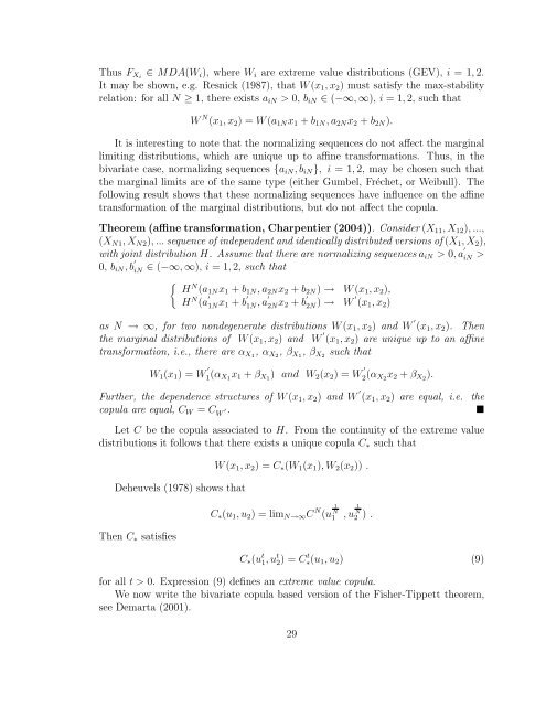
Thus F Xi 2 MDA(W i ), where W i are extreme value distributions (GEV), i =1; 2.It may be shown, e.g. Resnick (1987), that W (x 1 ;x 2 ) must satisfy the max-stabilityrelation: for all N ¸ 1, there exists a iN > 0, b iN 2 (¡1; 1), i =1; 2, such thatW N (x 1 ;x 2 )=W (a 1N x 1 + b 1N ;a 2N x 2 + b 2N ):It is interesting to note that the normalizing sequences do not a®ect the marginallimiting distributions, which are unique up to a±ne transformations. Thus, in thebivariate case, normalizing sequences fa iN ;b iN g; i =1; 2,maybechosensuchthatthe marginal limits are of the sametype(eitherGumbel,Frechet, or Weibull). Thefollowing result shows that these normalizing sequences have in°uence on the a±netransformation of the marginal distributions, but do not a®ect the copula.Theorem (a±ne transformation, Charpentier (2004)). Consider (X 11 ;X 12 );:::;(X N1 ;X N2 ); ::: sequence of independent and identically distributed versions of (X 1 ;X 2 ),with joint distribution H. Assume that there are normalizing sequences a iN > 0;a 0 iN >0, b iN ;b 0 iN 2 (¡1; 1), i =1; 2, such that½ H N (a 1N x 1 + b 1N ;a 2N x 2 + b 2N ) ! W (x 1 ;x 2 );H N (a 0 1N x 1 + b 0 1N ;a0 2N x 2 + b 0 2N ) ! W 0 (x 1 ;x 2 )as N !1, for two nondegenerate distributions W (x 1 ;x 2 ) and W 0 (x 1 ;x 2 ). Thenthe marginal distributions of W (x 1 ;x 2 ) and W 0 (x 1 ;x 2 ) areuniqueuptoana±netransformation, i.e., there are ® X1 , ® X2 , ¯X1 , ¯X2 such thatW 1 (x 1 )=W 0 1 (® X 1x 1 + ¯X1 ) and W 2 (x 2 )=W 0 2 (® X 2x 2 + ¯X2 ):Further, the dependence structures of W (x 1 ;x 2 ) and W 0 (x 1 ;x 2 ) are equal, i.e. thecopula are equal, C W = C W0 . ¥Let C be the copula associated to H. From the continuity of the extreme valuedistributions it follows that there exists a unique copula C ¤ such thatDeheuvels (1978) shows thatThen C ¤ satis¯esW (x 1 ;x 2 )=C ¤ (W 1 (x 1 );W 2 (x 2 )) :C ¤ (u 1 ;u 2 )=lim N!1 C N (u 1 N1 ;u 1 N2 ) :C ¤ (u t 1;u t 2)=C t ¤(u 1 ;u 2 ) (9)for all t>0. Expression (9) de¯nes an extreme value copula.We now write the bivariate copula based version of the Fisher-Tippett theorem,see Demarta (2001).29