Spatial Correlation of Historical Salmon Spawning Sites to Historical ...

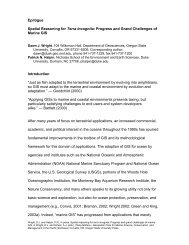
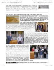
Spatial Correlation of Historical Salmon Spawning Sites toHistorical Splash Dam Locations in the Oregon Coast RangeBy Rebecca MillerGeo 565 Option 2 FinalIntroductionPhoto 1: Assen Brothers Splash Dam in 1912, Middle Creek Oregon. Photo courtesy of Coos County Historical SocietySplash dams were a tool used to transport timber in Oregon between 1880’s‐1957. The dams spannedthe width of the stream (Photo 1) and timber would accumulate behind the dam; loggers would releasethe spillway and the logs would float to downstream mills. Historical anecdotal and photographicevidence suggests in concurrent with log ‘splashes’, stream substrates such as gravels and cobbles werewashed away.…the stream environment was often adversely affected by splashing. Moving logs gougedfurrows in the gravel and many instances the suddenly increased flows scoured or moved thegravel bars, leaving only barren bedrock or heavy boulders…Dam operators have stated that fishruns reaching the dams were reduced within 3‐4 years after initial construction (Wendler 1955).

2In‐channel substrates are critical for successful for salmon redd building and spawning. The Oregon FishCommission, later known as Oregon Department of Fish and Wildlife (ODFW), began coho salmon(Oncorhynchus kisutch) spawning surveys in 1948. At that time, standard protocol called for ODFW toselect reliable sites that were known to be good spawning areas (Jacobs and Cooney, 1997). Since thespawning areas were spatially selected as being reliably productive, we can use this fact to see if there isany spatial correlation between the location of these historically reliable spawning areas and splash damsites.Study ImportanceMuch literature (Allen, 2004, Swetnam, 1999, Foster, 2003) cites the operation of splash dams instreams as one of the key culprits in the decline in salmonid populations through anecdotal evidenceand ‘rural legends.’ Yet, there have been no quantitative landscape level study to assess theenvironmental legacy impacts of splash dams.Data AnalysisGoal 1: To determine spatially if there is a disproportionate amount of historical spawningsurvey sites located in non‐splashed areas to splashed areas. This will be done by creating a densityanalysis of splash dams and overlaying the density polygon to stream survey sites.Goal 2: To determine if there is a lower total count of spawners located in splashed areasbetween 1950‐1970. This will be done by comparing the total spawners between all splashed sites toun‐splashed sites with a similar basin area and gradient. Spawning Surveys located within 4 km of asplash dam site or paired non‐splashed basin will be included. (The 4 km is along the splash dammedmainstem stream network, and does not follow up tributaries)

3DatasetsSplash Dams Data Layer‐ Western Oregon splash dam sites were located by searching 14museums and 2 courthouses for literature documentation, historical maps, and photographs.We conducted interviews with current & retired fisheries biologists, local historians and onesplash dam operator. Splash dam locations were mapped as a point and attributes were enteredinto a geodatabase using Arc/View 9.3. Data points were mapped at the Oregon LambertProjection, 1:24,000 scale.ODFW Spawning Survey Index Sites‐ A shape file (lines) of all spawning survey sites was obtainedfrom ODFW. In the attribute table, each survey line has an associated ID number, this IDnumber corresponds to an Excel table that summarizes spawning counts for each year,categorized as Adults and Jacks. I chose the earliest 20 year period (1950‐1970) to splashdamming operations, because 1) the closer in time the data sets are to splashing, there will be agreater chance to see a difference due to the splashing itself and not other factors such as elNiño (although presumably all populations would experience el Niño similarly) 2) protocolsslightly changed in the 1970’s, with many sites removed due to budget cuts. Data was projectedto Oregon Lambert.Coastal Landscape Analysi and Modeling Streams (CLAMS)‐ A US Forest Service stream layerderived from 10m DEM’s and calculated channel slope and basin area. This dataset is includedas ancillary data to compare splashed and non‐splashed areas of similar basin area and channelslope. Basin Area and channel slope are important covariates in describing physical channelconditions.

5Goal 2: To determine if there is a lower total count of spawners located in splashed areas between 1950‐1970.Step 1‐ Prepare the data for study area: Splash dam location layer was CLIPPED to ODFWhistorical stream survey study area (west crest of Coast Range).Step 2‐ ODFW excel spreadsheet ID numbers and data were transposed. A SPATIAL JOIN addedthe excel table to ODFW historical stream survey line layer.Step 3‐ All splash dam sites were BUFFERED by 4000m.Step 4‐ ’Select by Location’ was used to locate all spawning surveys located within 4000m allsplash dam sites buffer.Step 5‐ Measure tool was used to calculate final distance between the splash dam and spawningsurvey site along the mainstem stream network. If measure tool found that the distance alongthe network was greater than 4000m, the site was excluded from analysis.Step 6: For every splashed basin that met the inclusion criteria, identify a paired non‐splashedbasin of similar Basin Area and Channel Slope. The ‘Select by Attributes’ function was used onthe CLAMS data layer, for all stream network lines +/‐ 10 km2 of paired non‐splashed basin.Step 7: Selected network lines were buffered by 4000m.Step 8: ‘Select by Location’ function for historical spawning survey located within the nonsplashed4000m buffer.Step 9: If multiple spawning surveys were found with the same basin area size, the spawning siteclosest to the splash site was used. (1 st law in geography)Step 10: Repeat Step 6‐10, to pair every splashed basin to a non‐splashed basin.Step 11: Summarize total number of spawners/mile in splashed basins to un‐splashed basins.

6Results:Goal 1: To determine spatially if there is a disproportionate amount of historical spawning surveysites located in non‐splashed areas to splashed areas.There were 6 coho spawning surveys in the High Density, 16 in the Medium Densityclassification, and 12 in the Low Density (Map 1).

Map 1: Splash Dam Density and Historical Spawning Sites7

8Goal 2: To determine if there is a lower total count of spawners located in splashed areasbetween 1950‐1970.The spatial query found 3 of 121 splash dams that were located within 4km of a historicalspawning area (Table 1). I was able to match 2 splashed sites to 2 un‐splashed sites. No pairingwas found for the 3 rd splash dam site –N.F. Coquille, as the basin area was so large that nomatching non‐splashed spawning area existed (Map 2).Splashed Creek Basin Area Gradient Non‐Splashed Creek Basin Area Gradient(Paired)Steel Creek 10.2 0.01 Larson Creek 8.1 0.01N.F. Coquille 73.68 0.002 ‐ ‐ ‐Marlow Creek 17.33 0.01 Schonfield Creek 16.76 0.003Table 1: Physical Characteristics of paired splashed and non‐splashed basinsThere was more than twice the total number of coho spawners between 1950‐1970 in splashedbasin than non‐splashed basins (Table 2, Map 2). On average, there were 937 more totalspawners per mile in un‐splashed basins than splashed basins.Splashed CreekTotal Number ofSpawners between1950‐1970/mileNon‐Splashed Creek(Paired)Total Number ofSpawners between1950‐1970/mileMeanDifferenceSteel Creek 915 Larson Creek 1545 630Marlow Creek 527 Schonfield Creek 1773 1246Sum 1442 3317 1875Average 721 1658 937Table 2: Number of Spawners in splashed and non‐splashed basins

9Map2: Splash basins and paired non‐splashed basins located within 4000m of a historical stream surveyDiscussion/Sources of ErrorGoal 1: To determine spatially if there is a disproportionate amount of historical spawning survey siteslocated in non‐splashed areas to splashed areas.It does not visually appear that there is a spatial correlation between historical splash dam sites andhistorically abundant coho spawning sites. There was a disproportionate amount of historical spawningsites in low density sites (12) than high density sites (6). However, the total numbers do not reflect thewhole story. One source of error is that a greater area of the coast range is in the low density category,

10so naturally there are more spawning survey sites (12 in total) in the low density category. Similarly,only a small area is in the high density category, so there are far fewer spawning surveys (6 in total).The splash dam density classification of H, M, L changes slightly when splash dams east of the CoastRange crest are included (In the analysis only the west crest was used, as this was the study area ofspawning surveys). When splash dams found on both crests of the Cost Ranger are included, a highdensity patch is located in the central coast (Figure 3). With the inclusion of the east crest splash dams,area, the number of splash dams in each density classification changes to Low=9, Medium=19 andHigh=6.Figure 3: Density comparison with W. Crest and All Splash Dam sites

11Goal 2: To determine if there is a lower total count of spawners located in splashed areas between 1950‐1970.A result of more than twice the amount of spawners was counted in non‐splashed creeks. Conceptuallyand theoretically, one would expect to see a difference, but to actually see such a large quantitativemean difference result was rather exciting. However, this excitement should be tempered with a bit ofcaution. The coverage of spawning sites, didn’t match up as well as I would have liked, and this resultedin a small sample size. Only 3 of the 34 spawning survey sites match with splash dam sites, this low ratioof matched sites could be due to Coho biology as spawning areas tend to be in smaller tributaries whilesplash dams are located on larger mainstem creeks. The small sample size (2 pairs) may not reflect thetrue pattern of the number of spawners in splashed and unsplashed basins. It is possible that the 2 unsplashedsites for the paired basin comparison, (Larson and Schonfield Creeks) are not representative.One confounding variable is that the matched un‐splashed creeks themselves are spatially located closerto the ocean, so salmon don’t have to migrate as far to spawn. Two physical parameters that were notincluded, land use cover or basin geology, might also influence result. One unknown that should beinvestigated is where historical hatchery supplementation occurred.

12References:Allen, J. D. (2004) Landscapes and Riverscapes: The Influence of Land Use on Stream Ecosystems. AnnualReview of Ecology, Evolution, and Systematics, 35, 257‐284.Foster, D., Frederick Swanson, John Aber, Ingrid Burke, Nicholas Brokaw, David Tilman, Alan Knapp(2003) The Importance of Land‐Use Legacies to Ecology and Conservation. BioScience, 53, 77‐88.Jacobs, S. E., C.X. Cooney (1997) Oregon coastal salmon spawning surveys, 1994 and 1995. (ed F. D.Oregon Department of Fish and Wildlife). Portland.Swetnam, T. W., Craig D. Allen, Julio L. Betancourt (1999) Applied historical ecology: using the past tomanage for the future. Ecological Applications, 9, 1189‐1206.Wendler, H. O., G. Deschamps (1955) Logging dams on coast Washington streams, WSDF, Olympia.Data Sets:Coastal Landscape and Analysis Modeling Study (CLAMS). 2000. USDA Forest Service, Pacific NorthwestResearch Station. http://www.fsl.orst.edu/clamsMiller, Rebecca. 2010. Western Oregon Splash Dams between 1880‐1957.Oregon Department of Fish and Wildlife. Spawning Survey Index Sites 1948‐2008.http://oregonstate.edu/dept/ODFW/spawn/index.htm