Multi-component vortices in coupled NLS equations - Dmitry ...

Multi-component vortices in coupledNLS equationsDmitry Pelinovsky (McMaster University, Canada)Joint work with Anton Desyatnikov (Australian National University)and Jianke Yang (University of Vermont)Reference: Fundamentalnaya i prikladnaya matematika 12, 35–63 (2006)Conference "Symmetries in equations of mathematical physicsKiev, June 25-28, 2007

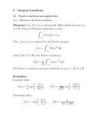
Scalar vorticesMain model: Focusing two-dimensional NLS equationiu t + u xx + u yy + f(|u| 2 )u = 0,where f(s) is C 1 (R + ) and f ′ (s) > 0 on s ∈ R + .Definition: Vortices are stationary solutions of the formu = R(r)e imθ e iωtwhere (r,θ) are polar coordinates on R 2 , m ∈ N is the vortexcharge and R(r) is a solution of the second-order ODE:R ′′ + 1 r R′ − m2r 2 R − ωR + f(R2 )R = 0,such that R(r) → r |m| as r → 0 and R(r) → e −√ ωr / √ r as r → ∞.

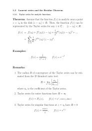
ExamplesSaturable medium with f(s) = s/(1 + s)Cubic-quintic approximation f(s) = s − s 2Desyatnikov, Kivshar, and Torner, Optical Vortices and VortexSolitons, In: Progress in Optics 47, Ed. E. Wolf (2005)

Typical instabilitiesVortices with charges m = 1 and m = 2 are unstable in the cubicNLS model:Skryabin and Firth, Phys. Rev. E 58, 3916 (1998)

Coupled NLS equationsWe consider the system of n coupled NLS equationsi ˙ψ k + ∆ψ k = W ′ (E)ψ k ,k = 1, 2,...,n,where ψ k : R 2 × R ↦→ C and W : R + ↦→ R + is C 2 -function ofE = ∑ nk=1 |ψ k| 2 . The system is Hamiltonian with∫ [ n∑(( n∑)]H = |∂x ψ k | 2 + |∂ y ψ k | 2) + W |ψ k | 2 dxdyR 2 k=1k=1Vector momentum, angular momentum, and the charges∫Q k = |ψ k | 2 dxdy, k = 1,...,nR 2are basic conserved quantities of the system.

Symplectic symmetriesThe Hamiltonian function is invariant with respect to N-parametergroup of rotations in the space R 2n or C n × ¯C n , where( )2n (2n)!N = = = n(2n − 1).2 2!(2n − 2)!Let G be a linear transformation in x ∈ R 2n and J be the symplecticmatrix such that ẋ = Jgrad(H(x)). Then, the Hamiltonian systemis invariant under the linear transformation if and only ifJ = GJG TSuch transformations G are called symplectic transformations. IfG = I + g, then gJ + Jg T = 0.

Symmetries of the coupled NLSLemma: The group of symplectic rotations in R 2n is generated bythe n 2 -parameter matrix( )A Bg = ,−B T Awhere A T = −A and B T = B. Equivalently, the group ofsymplectic rotations in C n is generated by g = A − iB.Additional conserved quantities related to the symmetries:∫Q k,m = ψ k ¯ψm dxdy, k = 1,...,n, m = k,...,n,R 2where n quantities are real-valued charges Q k = Q k,k andn(n − 1)/2 quantities Q k,m with m ≠ k are complex-valued.

where (α 1 ,α 2 ) are complex-valued parameters and (θ 1 ,θ 2 ) arereal-valued parameters.Example n = 2Symplectic rotations in C 2G 3 =(( )e iθ 10G 1 =0 1)cosθ 3 sin θ 3, G 4 =− sin θ 3 cosθ 3, G 2 =((1 00 e iθ 2))cosθ 4 i sin θ 4,i sin θ 4 cos θ 4where θ 1,2,3,4 are defined on [0, 2π]. If (ψ 1 ,ψ 2 ) is a solution of thecoupled NLS equations, then a new solution ( ˜ψ 1 , ˜ψ 2 ) is˜ψ 1 = α 1 e iθ 1ψ 1 + α 2 e iθ 2ψ 2 ,˜ψ 2 = −ᾱ 2 e iθ 1ψ 1 + ᾱ 1 e iθ 2ψ 2 ,

Stationary solutions : classificationConsider the stationary solution in the form:ψ k = ϕ k (x)e iω kt ,k = 1,...,n,where ω k is real-valued parameter and ϕ k (x) solves∆ϕ k − ω k ϕ k = W ′ (E)ϕ kFirst Alternative:For any k ≠ m, either (I) ω k = ω m or (II) (ϕ k ,ϕ m ) = 0.Class I contains a variety of super-symmetric vortex congifurations.Class II contains a variety of coupled states between solitons andvortices of different frequencies.

Vortex solutions of class ISeparating the polar coordinates (r,θ) in R 2 :ϕ k = φ k (θ)R k (r),k = 1,...,n,we obtain two ODEs:φ ′′k + m 2 kφ k = 0, R ′′k + 1 r R′ k − m2 kr 2 R k = (W ′ (E 0 ) + ω)R k ,where E 0 (r) = ∑ nk=1 R2 k (r)|φ k(θ)| 2 . By the periodicity of φ k (θ),parameter m k is integer (vortex charge).Second Alternative:For any k ≠ m, either (i) m 2 k = m2 m, R k = R m or (ii)∫ ∞0R k (r)R m (r)dr/r = 0, φ k (θ) = e ±im kθ .

Vortex solutions of sub-class I (i)Let m 2 k = m2 and R k = R(r) ∀k, whereThen,R ′′ + 1 r R′ − m2r 2 R = (W ′ (R 2 ) + ω)R.φ k = a k e imθ + b k e −imθ ,k = 1,...,n,subject to the solvability constraint ∑ nk=1 |φ k| 2 = 1, which isequivalent to the normalization in C n :‖a‖ 2 + ‖b‖ 2 = 1, (a,b) = 0,where a = (a 1 ,...,a n ) T and b = (b 1 ,...,b n ) T are in C n .

Examples for n = 2• If b = 0, then the solution is vortex pair of double charge:ϕ 1 = a 1 R(r)e imθ , ϕ 2 = a 2 R(r)e imθ ,which is equivalent to the scalar vortex a = (1, 0) T bysymplectic rotations• If a = 1 √2(1, 0) T and b = 1 √2(0, 1) T , then the solution is vortexpair of hidden charge:ϕ 1 = 1 √2R(r)e imθ , ϕ 2 = 1 √2R(r)e −imθ .which generates a family with a,b ≠ 0 by symplectic rotations

Examples for n = 2Cubic model(Manakov model)Cubic–quntic model

Vortex solutions of sub-class I (ii)Let φ k (θ) = e ±imkθ with m 2 k being distinct for all k. There exists aninvariant manifold R k (r) ≡ 0 for any k.A hierarchy of vortex states:• Scalar vortex• Two-charge vortexϕ 1 = R(r)e imθ , ϕ k = 0, k = 2,...,n.ϕ 1 = α 1 R 1 (r)e im 1θ , ϕ 2 = α 2 R 2 (r)e im 2θ , ϕ k = 0, k = 3,...n,where R 1,2 (r) solve L m1 R 1 = 0 and L m2 R 2 = 0 withL m = d2dr 2 + 1 rddr − m2r 2 − ω + W ′ (R 2 1 + R 2 2).

Examples for n = 2Cubic (Manakov) system(a) (m 1 ,m 2 ) = (0, 1), (b) (m 1 ,m 2 ) = (0, 2), (c) (m 1 ,m 2 ) = (1, 2).Conjecture from the numerical observations:|m 1 | + n 1 = |m 2 | + n 2 ,where n k is the number of nodes of R k (r) on r > 0.

Symmetries and linearizationStability problem for perturbation vector (u,w) ∈ C 2n is( ) ( ) ( )u I O uH = iλ,v O −I vwhereH = (−∆ + W ′ (E))(I OO I)+ W ′′ (E)(ϕ¯ϕ)· (¯ϕ T ϕ T)and E(x) = ∑ nk=1 |ϕ k(x)| 2 .Remark: The last term in H is the outer product, which is a rank-onematrix for any x ∈ R 2 . This can be used for block-diagonalizationand simplification of the stability problem.

Example: vortices of sub-class I(ii)For instance, consider a scalar vortex:ϕ k (x) = a k R(r)e imθ , a k ∈ C :n∑k=1|a k | 2 = 1An ortho-normal basis in C n : S 1 = {a,c 1 ,c 2 ,...,c n−1 }, where{c j } n−1j=1 spans the orthogonal compliment of a. The decompositionu(x) = α + (x)a +∑n−1j=1γ + j (x)c j, v(x) = α − (x)a +∑n−1j=1γ − j (x)c jblock-diagonalizes H into 2-by-2 coupled non-self-adjoint problemfor (α + ,α − ) and pairs of uncoupled self-adjoint problems for{γ + j ,γ− j }n−1 j=1 .

Example: vortices of sub-class I(i)For instance, consider a vortex pair with hidden chargesuch thatϕ k (x) = ( a k e imθ + b k e −imθ) R(r), a k ,b k ∈ C,(a,b) = 0, ‖a‖ 2 = 1 + µ2, ‖b‖ 2 = 1 − µ .2A similar decomposition over an ortho-normal basisS 2 = {a,b,c 1 ,...,c n−2 } ⊂ C n block-diagonalizes H into 4-by-4coupled non-self-adjoint problem and pairs of uncoupledself-adjoint problems.

Example: instabilities of vortex pairs(a) µ = ±1 - vortex of double charge(b) µ = 0 - vortex of hidden charge

Conclusion• Analysis of symplectic rotations and conserved quantities• Classification and simplification of exact vortex solutions andtheir linearizations in the system of coupled NLS equations• An algorithm for analysis of a particular family of solutions1. Construct the seed vortex for a given vortex solution2. Study analytically and numerically the associatedlinearization problem for the seed vortex3. Rotate the seed vortex and the eigenvectors of the linearizedproblem with the same group of symplectic rotations toobtain relevant results for the given vortex.• Nonlinear dynamics of solutions along the family of symplecticrotations is not yet well understood.