A Simulated Annealing Based Multi-objective Optimization Algorithm ...

2exploration along the front. However, a proper choice of thew i s remains challenging task.In addition to the earlier aggregating approaches of multiobjectiveSA, there have been a few techniques that incorporatethe concept of Pareto-dominance. Some such methodsare proposed in [16], [17] which use Pareto-domination basedacceptance criterion in multi-objective SA. A good reviewof several multi-objective simulated annealing algorithms andtheir comparative performance analysis can be found in [18].Since the technique in [17] has been used in this article forthe purpose of comparison, it is described in detail later.In Pareto-domination-based multi-objective SAs developedso far, the acceptance criterion between the current and a newsolution has been formulated in terms of the difference in thenumber of solutions that they dominate [16], [17]. The amountby which this domination takes place is not taken into consideration.In this article, a new multi-objective SA is proposed,hereafter referred to as AMOSA (Archived Multi-objectiveSimulated Annealing), which incorporates a novel concept ofamount of dominance in order to determine the acceptanceof a new solution. The PO solutions are stored in an archive.A complexity analysis of the proposed AMOSA is provided.The performance of the newly proposed AMOSA is comparedto two other well-known MOEA’s, namely NSGA-II [19] andPAES [20] for several function optimization problems whenbinary encoding is used. The comparison is made in termsof several performance measures, namely Convergence [19],Purity [21], [22], Spacing [23] and MinimalSpacing [21].Another measure called displacement [8], [24], that reflectsboth the proximity to and the coverage of the true PO front,is also used here for the purpose of comparison. This measureis especially useful for discontinuous fronts where we canestimate if the solution set is able to approximate all the subfronts.Many existing measures are unable to achieve this.It may be noted that the multi-objective SA methods developedin [16], [17] are on lines similar to ours. The concept ofarchive or a set of potentially PO solutions is also utilized in[16], [17] for storing the non-dominated solutions. Instead ofscalarizing the multiple objectives, a domination based energyfunction is defined. However there are notable differences.Firstly, while the number of solutions that dominate the newsolution x determines the acceptance probability of x in theearlier attempts, in the present article this is based on theamount of domination of x with respect to the solutions inthe archive and the current solution. In contrast to the worksin [16], [17] where a single form of acceptance probabilityis considered, the present article deals with different forms ofacceptance probabilities depending on the domination status,the choice of which are explained intuitively later on.In [17] an unconstrained archive is maintained. Note thattheoretically, the number of Pareto-optimal solutions can beinfinite. Since the ultimate purpose of an MOO algorithm isto provide the user with a set of solutions to choose from, it isnecessary to limit the size of this set for it to be usable by theuser. Though maintaining unconstrained archives as in [17] isnovel and interesting, it is still necessary to finally reduce itto a manageable set. Limiting the size of the population (asin NSGA-II) or the Archive (as in AMOSA) is an approachin this direction. Clustering appears to be a natural choice forreducing the loss of diversity, and this is incorporated in theproposed AMOSA. Clustering has also been used earlier in[25].For comparing the performance of real-coded AMOSAwith that of the multi-objective SA (MOSA) [17], six threeobjective test problems, namely, DTLZ1-DTLZ6 are used.Results demonstrate that the performance of AMOSA iscomparable to, often better than, that of MOSA in terms ofPurity, Convergence and Minimal Spacing. Comparison is alsomade with real-coded NSGA-II for the above mentioned sixproblems, as well as for some 4, 5, 10 and 15 objective testproblems. Results show that the performance of AMOSA issuperior to that of NSGA-II specially for the test problemswith many objective functions. This is an interesting and themost desirable feature of AMOSA since Pareto ranking-basedMOEAs, such as NSGA-II [19] do not work well on manyobjectiveoptimization problems as pointed out in some recentstudies [26], [27].II. MULTI-OBJECTIVE ALGORITHMSThe multi-objective optimization can be formally statedas follows [1]. Find the vectors x ∗ = [x ∗ 1, x ∗ 2, . . . , x ∗ n] T ofdecision variables that simultaneously optimize the M objectivevalues {f 1 (x), f 2 (x), . . . , f M (x)}, while satisfying theconstraints, if any.An important concept of multi-objective optimization is thatof domination. In the context of a maximization problem, a solutionx i is said to dominate x j if ∀k ∈ 1, 2, . . . , M, f k (x i ) ≥f k (x j ) and ∃k ∈ 1, 2, . . . , M, such that f k (x i ) > f k (x j ).Among a set of solutions P , the nondominated set of solutionsP ′are those that are not dominated by any member of theset P . The non-dominated set of the entire search space S isthe globally Pareto-optimal set. In general, a multi-objectiveoptimization algorithm usually admits a set of solutions thatare not dominated by any solution encountered by it.A. Recent MOEA algorithmsDuring 1993-2003, a number of different evolutionary algorithmswere suggested to solve multi-objective optimizationproblems. Among these, two well-known ones namely, PAES[20] and NSGA-II [19], are used in this article for the purposeof comparison. These are described in brief.Knowles and Corne [20] suggested a simple MOEA usinga single parent, single child evolutionary algorithm, similar to(1+1) evolutionary strategy. Instead of using real parameters,binary strings and bit-wise mutation are used in this algorithmto create the offspring. After creating the child and evaluatingits objectives, it is compared with respect to the parent. If thechild dominates the parent, then the child is accepted as thenext parent and the iteration continues. On the other hand ifparent dominates the child, the child is discarded and a newmutated solution (a new solution) is generated from the parent.However if the parent and the child are nondominating to eachother, then the choice between the child and the parent isresolved by comparing them with an archive of best solutionsfound so far. The child is compared with all members of the

3archive to check if it dominates any member of the archive.If yes, the child is accepted as the new parent and all thedominated solutions are eliminated from the archive. If thechild does not dominate any member of the archive, both theparent and the child are checked for their nearness with thesolutions of the archive. If the child resides in a less crowdedregion in the parameter space, it is accepted as a parent and acopy is added to the archive. Generally this crowding conceptis implemented by dividing the whole solution space into d Msubspaces where d is the depth parameter and M is the numberof objective functions. The subspaces are updated dynamically.The other popular algorithm for multi-objective optimizationis NSGA-II proposed by Deb et al. [19]. Here, initiallya random parent population P 0 of size N is created. Thenthe population is sorted based on the non-domination relation.Each solution of the population is assigned a fitness whichis equal to its non-domination level. A child population Q 0is created from the parent population P 0 by using binarytournament selection, recombination, and mutation operators.Generally according to this algorithm, initially a combinedpopulation R t = P t + Q t is formed of size R t , which is 2N.Now all the solutions of R t are sorted based on their nondominationstatus. If the total number of solutions belongingto the best non-dominated set F 1 is smaller than N, F 1is completely included into P (t+1) . The remaining membersof the population P (t+1) are chosen from subsequent nondominatedfronts in the order of their ranking. To chooseexactly N solutions, the solutions of the last included frontare sorted using the crowded comparison operator and the bestamong them (i.e., those with larger values of the crowdingdistance) are selected to fill in the available slots in P (t+1) .The new population P (t+1) is now used for selection, crossoverand mutation to create a new population Q (t+1) of size N,and the process continues. The crowding distance operator isalso used in the parent selection phase in order to break a tiein the binary tournament selection. This operator is basicallyresponsible for maintaining diversity in the Pareto front.B. Recent MOSA algorithm [17]One of the recently developed MOSA algorithm is by Smithet al. [17]. Here a dominance based energy function is used. Ifthe true Pareto front is available then the energy of a particularsolution x is calculated as the total number of solutions thatdominates x. However as the true Pareto front is not availableall the time a proposal has been made to estimate the energybased on the current estimate of the Pareto front, F ′ , whichis the set of mutually non-dominating solutions found thusfar in the process. Then the energy of the current solution xis the total number of solutions in the estimated front whichdominates x. If ‖F ′ ′ ‖ is the energy of the new solution x′xand ‖F x‖ ′ is the energy of the current solution x, then energydifference between the current and the proposed solution iscalculated as δE(x ′ , x) = (‖F ′ ‖ − ‖F ′ x ′ x ‖)/‖F ′ ‖. Division by‖F ′ ‖ ensures that δE is always less than unity and providessome robustness against fluctuations in the number of solutionsin F ′ . If the size of F ′is less than some threshold, thenattainment surface sampling method is adopted to increase thenumber of solutions in the final Pareto front. Authors haveperturbed a decision variable with a random number generatedfrom the laplacian distribution. Two different sets of scalingfactors, traversal scaling which generates moves to a nondominatedproposal within a front, and location scaling whichlocates a front closer to the original front, are kept. Thesescaling factors are updated with the iterations.III. ARCHIVED MULTI-OBJECTIVE SIMULATEDANNEALING (AMOSA)As mentioned earlier, the AMOSA algorithm is based onthe principle of SA [3]. In this article at a given temperatureT , a new state, s, is selected with a probabilityp qs =1−(E(q,T )−E(s,T ))1 + e T, (1)where q is the current state and E(s, T ) and E(q, T ) are thecorresponding energy values of s and q, respectively. Note thatthe above equation automatically ensures that the probabilityvalue lies in between 0 and 1. AMOSA incorporates theconcept of an Archive where the non-dominated solutionsseen so far are stored. In [28] the use of unconstrainedArchive size to reduce the loss of diversity is discussed indetail. In our approach we have kept the archive size limitedsince finally only a limited number of well distributed Paretooptimalsolutions are needed. Two limits are kept on the sizeof the Archive: a hard or strict limit denoted by HL, anda soft limit denoted by SL. During the process, the nondominatedsolutions are stored in the Archive as and whenthey are generated until the size of the Archive increases toSL. Thereafter if more non-dominated solutions are generated,these are added to the Archive, the size of which is thereafterreduced to HL by applying clustering. The structure of theproposed simulated annealing based AMOSA is shown inFigure 1. The parameters that need to be set a priori arementioned below.• HL: The maximum size of the Archive on termination.This set is equal to the maximum number of nondominatedsolutions required by the user.• SL: The maximum size to which the Archive may be filledbefore clustering is used to reduce its size to HL.• Tmax: Maximum (initial) temperature.• Tmin: Minimal (final) temperature.• iter: Number of iterations at each temperature.• α: The cooling rate in SAThe different steps of the algorithm are now explained indetail.A. Archive InitializationThe algorithm begins with the initialization of a numberγ× SL (γ > 1) of solutions. Each of these solutions isrefined by using a simple hill-climbing technique, acceptinga new solution only if it dominates the previous one. Thisis continued for a number of iterations. Thereafter the nondominatedsolutions (ND) that are obtained are stored in theArchive, up to a maximum of HL. In case the number ofnondominated solutions exceeds HL, clustering is applied to

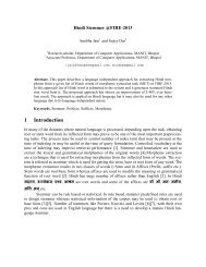
4Algorithm AMOSASet Tmax, Tmin, HL, SL, iter, α, temp=Tmax.Initialize the Archive.current-pt = random(Archive). /* randomly chosen solution from the Archive*/while (temp > Tmin)for (i=0; i< iter; i++)new-pt=perturb(current-pt).Check the domination status of new-pt and current-pt./* Code for different cases */if (current-pt dominates (∑ new-pt) /* Case 1*/ki,new−pt)i=1∆dom avg =∆dom +∆dom current−pt,new−pt.(k+1)/* k=total-no-of points in the Archive which dominate new-pt, k ≥ 0. */1prob=.1+exp(∆dom avg∗temp)Set new-pt as current-pt with probability=probif (current-pt and new-pt are non-dominating to each other) /* Case 2*/Check the domination status of new-pt and points in the Archive.if (new-pt is dominated by k (k ≥1) points in the Archive) /* Case 2(a)*/prob=∆dom avg =11+exp(∆dom (∑ .avg∗temp)ki,new−pt)i=1 ∆domk.Set new-pt as current-pt with probability=prob.if (new-pt is non-dominating w.r.t all the points in the Archive) /* Case 2(b)*/Set new-pt as current-pt and add new-pt to the Archive.if Archive-size > SLCluster Archive to HL number of clusters.if (new-pt dominates k, (k ≥1) points of the Archive) /* Case 2(c)*/Set new-pt as current-pt and add it to the Archive.Remove all the k dominated points from the Archive.if (new-pt dominates current-pt) /* Case 3 */Check the domination status of new-pt and points in the Archive.if (new-pt is dominated by k (k ≥1) points in the Archive) /* Case 3(a)*/∆dom min = minimum of the difference of domination amounts between the new-ptand the k points11+exp(−∆dom min ) .prob=Set point of the archive which corresponds to ∆dom min as current-pt with probability=probelse set new-pt as current-pt.if (new-pt is non-dominating with respect to the points in the Archive) /* Case 3(b) */Set new-pt as the current-pt and add it to the Archive.if current-pt is in the Archive, remove it from the Archive.else if Archive-size> SL.Cluster Archive to HL number of clusters.if (new-pt dominates k other points in the Archive ) /* Case 3(c)*/Set new-pt as current-pt and add it to the Archive.Remove all the k dominated points from the Archive.End fortemp= α∗temp.End whileif Archive-size > SLCluster Archive to HL number of clusters.Fig. 1.The AMOSA Algorithmreduce the size to HL (the clustering procedure is explainedbelow). That means initially Archive contains a maximum ofHL number of solutions.In the initialization phase it is possible to get an Archive ofsize one. In MOSA [17], in such cases, other newly generatedsolutions which are dominated by the archival solution willbe indistinguishable. In contrast, the amount of dominationas incorporated in AMOSA will distinguish between “moredominated” and “less dominated” solutions. However, in futurewe intend to use a more sophisticated scheme, in line with thatadopted in MOSA.B. Clustering the Archive SolutionsClustering of the solutions in the Archive has been incorporatedin AMOSA in order to explicitly enforce the diversityof the non-dominated solutions. In general, the size of theArchive is allowed to increase up to SL (> HL), after whichthe solutions are clustered for grouping the solutions into HLclusters. Allowing the Archive size to increase upto SL notonly reduces excessive calls to clustering, but also enablesthe formation of more spread out clusters and hence betterdiversity. Note that in the initialization phase, clustering is

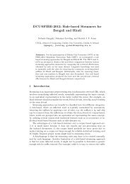
5executed once even if the number of solutions in the Archiveis less than SL, as long as it is greater than HL. This enables itto start with atmost HL non-dominated solutions and reducesexcessive calls to clustering in the initial stages of the AMOSAprocess.For clustering, the well-known Single linkage algorithm[29] is used. Here, the distance between any two clusterscorresponds to the length of the shortest link between them.This is similar to the clustering algorithm used in SPEA [25],except that they have used average linkage method [29]. AfterHL clusters are obtained, the member within each clusterwhose average distance to the other members is the minimum,is considered as the representative member of the cluster. Atie is resolved arbitrarily. The representative points of all theHL clusters are thereafter stored in the Archive.C. Amount of DominationAs already mentioned, AMOSA uses the concept of amountof domination in computing the acceptance probability of anew solution. Given two solutions a and b, the amount ofdomination is defined as∆dom a,b = ∏ M|f i(a)−f i(b)|i=1,f i(a)≠f i(b) R iwhere M = numberof objectives and R i is the range of the ith objective. Notethat in several cases, R i may not be known a priori. In thesesituations, the solutions present in the Archive along with thenew and the current solutions are used for computing it. Theconcept of ∆dom a,b is illustrated pictorially in Figure 2 fora two objective case. ∆dom a,b is used in AMOSA whilecomputing the probability of acceptance of a newly generatedsolution.f2AFig. 2. Total amount of domination between the two solutions A and B =the area of the shaded rectangleD. The Main AMOSA ProcessOne of the points, called current-pt, is randomly selectedfrom Archive as the initial solution at temperaturetemp=Tmax. The current-pt is perturbed to generate a newsolution called new-pt. The domination status of new-pt ischecked with respect to the current-pt and solutions in Archive.Based on the domination status between current-pt and newptthree different cases may arise. These are enumerated below.• Case 1: current-pt dominates the new-pt and k (k ≥ 0)points from the Archive dominate the new-pt.This situation is shown in Figure 3. Here Figure 3(a)Bf1and (b) denote the situations where k = 0 and k ≥ 1respectively. ( Note that all the figures correspond to atwo objective maximization problem.) In this case, thenew-pt is selected as the current-pt withprobability =11 + exp(∆dom avg ∗ temp) , (2)∑kwhere ∆dom avg =((i=1 ∆dom i,new−pt) + ∆dom current−pt,new−p1). Note that ∆dom avg denotes the average amount ofdomination of the new-pt by (k + 1) points, namely,the current-pt and k points of the Archive. Also, ask increases, ∆dom avg will increase since here thedominating points that are farther away from the new-ptare contributing to its value.Lemma: When k = 0, the current-pt is on the archivalfront.Proof: In case this is not the case, then some point, say A,in the Archive dominates it. Since current-pt dominatesthe new-pt, by transitivity, A will also dominate the newpt.However, we have considered that no other point in theArchive dominates the new-pt as k = 0. Hence proved.However if k ≥ 1, this may or may not be true.• Case 2: current-pt and new-pt are non-dominating withrespect to each other.Now, based on the domination status of new-pt andmembers of Archive, the following three situations mayarise.1) new-pt is dominated by k points in the Archivewhere k ≥ 1. This situation is shown in Figure 4(a).The new-pt is selected as the current-pt withprobability =1(1 + exp(∆dom avg ∗ temp)) , (3)where ∆dom avg = ∑ ki=1 (∆dom i,new−pt)/k. Notethat here the current-pt may or may not be on thearchival front.2) new-pt is non-dominating with respect to the otherpoints in the Archive as well. In this case the newptis on the same front as the Archive as shownin Figure 4(b). So the new-pt is selected as thecurrent-pt and added to the Archive. In case theArchive becomes overfull (i.e., the SL is exceeded),clustering is performed to reduce the number ofpoints to HL.3) new-pt dominates k (k ≥1) points of the Archive.This situation is shown in Figure 4(c). Again, thenew-pt is selected as the current-pt, and added tothe Archive. All the k dominated points are removedfrom the Archive. Note that here too the current-ptmay or may not be on the archival front.• Case 3: new-pt dominates current-ptNow, based on the domination status of new-pt andmembers of Archive, the following three situations mayarise.1) new-pt dominates the current-pt but k (k ≥ 1) pointsin the Archive dominate this new-pt. Note that thissituation (shown in Figure 5(a)) may arise only if the

6current-pt is not a member of the Archive. Here, theminimum of the difference of domination amountsbetween the new-pt and the k points, denoted by∆dom min , of the Archive is computed. The pointfrom the Archive which corresponds to the minimumdifference is selected as the current-pt with prob =11+exp(−∆dom min). Otherwise the new-pt is selectedas the current-pt. Note that according to the SAparadigm, the new-pt should have been selectedwith probability 1. However, due to the presenceof Archive, it is evident that solutions still betterthan new-pt exist. Therefore the new-pt and thedominating points in the Archive that is closest tothe new-pt (corresponding to ∆dom min ) competefor acceptance. This may be considered a formof informed reseeding of the annealer only if theArchive point is accepted, but with a solution closestto the one which would otherwise have survived inthe normal SA paradigm.2) new-pt is non-dominating with respect to the pointsin the Archive except the current-pt if it belongs tothe Archive. This situation is shown in Figure 5(b).Thus new-pt, which is now accepted as the currentpt,can be considered as a new nondominated solutionthat must be stored in Archive. Hence newptis added to the Archive. If the current-pt is inthe Archive, then it is removed. Otherwise, if thenumber of points in the Archive becomes more thanthe SL, clustering is performed to reduce the numberof points to HL.Note that here the current-pt may or may not be onthe archival front.3) new-pt also dominates k (k ≥ 1), other points, inthe Archive (see Figure 5(c)). Hence, the new-pt isselected as the current-pt and added to the Archive,while all the dominated points of the Archive areremoved. Note that here the current-pt may or maynot be on the archival front.The above process is repeated iter times for each temperature(temp). Temperature is reduced to α × temp, usingthe cooling rate of α till the minimum temperature, Tmin, isattained. The process thereafter stops, and the Archive containsthe final non-dominated solutions.Note that in AMOSA, as in other versions of multi-objectiveSA algorithms, there is a possibility that a new solution worsethan the current solution may be selected. In most otherMOEAs, e.g., NSGA-II, PAES, if a choice needs to be madebetween two solutions x and y, and if x dominates y, then xis always selected. It may be noted that in single objectiveEAs or SA, usually a worse solution also has a non-zerochance of surviving in subsequent generations; this leads toa reduced possibility of getting stuck at suboptimal regions.However, most of the MOEAs have been so designed that thischaracteristics is lost. The present simulated annealing basedalgorithm provides a way of incorporating this feature.E. Complexity AnalysisThe complexity analysis of AMOSA is provided in thissection. The basic operations and their worst case complexitiesare as follows:1) Archive initialization: O(SL).2) Procedure to check the domination status of any twosolutions: O(M), M = # objectives.3) Procedure to check the domination status between aparticular solution and the Archive members: O(M ×SL).4) Single linkage clustering: O(SL 2 × log(SL)) [30].5) Clustering procedure is executed• once after initialization if |ND| > HL• after each (SL−HL) number of iterations.• at the end if final |Archive| > HLSo maximum number of times the Clustering procedureis called=(TotalIter/(SL−HL))+2.Therefore, total complexity due to Clustering procedureis O((TotalIter/(SL−HL)) × SL 2 × log(SL)).Total complexity of AMOSA becomes(SL+M+M×SL)×(T otalIter)+ T otalIterSL − HL ×SL2 ×log(SL).(4)Let SL= β×HL where β ≥ 2 and HL = N where N isthe population size in NSGA-II and archive size in PAES.Therefore overall complexity of the AMOSA becomes(T otalIter) × (β × N + M + M × β × N + (β 2 /(β − 1))or,×N × log(βN)), (5)O(T otalIter × N × (M + log(N))). (6)Note that the total complexity of NSGA-II is O(TotalIter×M×N 2 ) and that of PAES is O(TotalIter ×M × N). NSGA-II complexity depends on the complexity of non-dominatedprocedure. With the best procedure, the complexity isO(TotalIter×M × N × log(N)).IV. SIMULATION RESULTSIn this section, we first describe comparison metrics used forthe experiments. The performance analysis of both the binarycodedAMOSA and real-coded AMOSA are also provided inthis section.A. Comparison MetricsIn multi-objective optimization, there are basically twofunctionalities that an MOO strategy must achieve regardingthe obtained solution set [1]. It should converge as close tothe true PO front as possible and it should maintain as diversea solution set as possible.The first condition clearly ensures that the obtained solutionsare near optimal and the second condition ensures thata wide range of trade-off solutions is obtained. Clearly, thesetwo tasks cannot be measured with one performance measureadequately. A number of performance measures have beensuggested in the past. Here we have mainly used three such

7f2 (maximize)f2(maximize)Points in the archivePoints in the archiveCurrentCurrentNewNewf1maximizef1(maximize)(a)(b)Fig. 3. Different cases when New is dominated by Current (a) New is non-dominating with respect to the solutions of Archive except Current if it is in thearchive (b) Some solutions in the Archive dominate Newf2(maximize)f2(maximize)f2(maximize)Points in the archivePoints in the archivePoints in the archieveCurrentCurrentNewCurrentNewNewf1(maximize)f1(maximize)(a) (b) (c)f1(maximize)Fig. 4. Different cases when New and Current are non-dominating (a) Some solutions in Archive dominates New (b) New is non-dominating with respectto all the solutions of Archive (c) New dominates k (k ≥ 1) solutions in the Archive .f2(maximize)f2(maximize)f2(maximize)Points in the archiveNewPoints in the archiveNewPoints in the archiveCurrentCurrentNewCurrentf1(maximize)f1(maximize)(a) (b) (c)f1(maximize)Fig. 5. Different cases when New dominates the Current (a) New is dominated by some solutions in Archive (b) New is non-dominating with respect to thesolutions in the Archive except Current, if it is in the archive (c) New dominates some solutions of Archive other than Currentperformance measures. The first measure is the Convergencemeasure γ [19]. It measures the extent of convergence of theobtained solution set to a known set of PO solutions. Lower thevalue of γ, better is the convergence of the obtained solutionset to the true PO front. The second measure called Purity [21],[22] is used to compare the solutions obtained using differentMOO strategies. It calculates the fraction of solutions from aparticular method that remains nondominating when the finalfront solutions obtained from all the algorithms are combined.A value near to 1(0) indicates better (poorer) performance.The third measure named Spacing was first proposed bySchott [23]. It reflects the uniformity of the solutions overthe non-dominated front. It is shown in [21] that this measurewill fail to give adequate result in some situations. In order toovercome the above limitations, a modified measure, namedMinimalSpacing is proposed in [21]. Smaller values of Spacingand MinimalSpacing indicate better performance.It may be noted that if an algorithm is able to approximateonly a portion of the true PO front, not its full extents, noneof the existing measures, will be able to reflect this. In caseof discontinuous PO front, this problem becomes severe whenan algorithm totally misses a sub-front. Here a performancemeasure which is very similar to the measure used in [8] and[24] named displacement is used that is able to overcomethis limitation. It measures how far the obtained solution setis from a known set of PO solutions. In order to compute

8displacement measure, a set P ∗ consisting of uniformlyspaced solutions from the true PO front in the objective spaceis found (as is done while calculating γ). Then displacementis calculated asdisplacement = 1|P ∗ ||P ∗ | × ∑(min |Q|j=1d(i, j)) (7)i=1where Q is the obtained set of final solutions, and d(i, j) isthe Euclidean distance between the ith solution of P ∗ and jthsolution of Q. Lower the value of this measure, better is theconvergence to and extent of coverage of the true PO front.B. Comparison of Binary Encoded AMOSA with NSGA-II andPAESFirstly, we have compared the binary encoded AMOSAwith the binary-coded NSGA-II and PAES algorithm. ForAMOSA binary mutation is used. Seven test problems havebeen considered for the comparison purpose. These are SCH1and SCH2 [1], Deb1 and Deb4 [31], ZDT1, ZDT2, ZDT6 [1].All the algorithms are executed ten times per problem andthe results reported are the average values obtained for theten runs. In NSGA-II the crossover probability (p c ) is keptequal to 0.9. For PAES the depth value d is set equal to 5.For AMOSA the cooling rate α is kept equal to 0.8. Thenumber of bits assigned to encode each decision variabledepends on the problem. For example in ZDT1, ZDT2 andZDT6 which all are 30-variable problems, 10 bits are used toencode each variable, for SCH1 and SCH2 which are singlevariable problems and for Deb1 and Deb4 which are twovariable problems, 20 bits are used to encode each decisionvariable. In all the approaches, binary mutation applied with aprobability of p m = 1/l, where l is the string length, is usedas the perturbation operation. We have chosen the values ofTmax (maximum value of the temperature), Tmin (minimumvalue of the temperature) and iter (number of iterations ateach temperature) so that total number of fitness evaluations ofthe three algorithms becomes approximately equal. For PAESand NSGA-II, identical parameter settings as suggested in theoriginal studies have been used. Here the population size inNSGA-II, and archive sizes in AMOSA and PAES are setto 100. Maximum iterations for NSGA-II and PAES are 500and 50000 respectively. For AMOSA, T max = 200, T min =10 −7 , iter = 500. The parameter values were determined afterextensive sensitivity studies, which are omitted here to restrictthe size of the article.1) Discussions of the Results: The Convergence and Purityvalues obtained using the three algorithms is shown in TableI. AMOSA performs best for ZDT1, ZDT2, ZDT6 and Deb1in terms of γ. For SCH1 all three are performing equally well.NSGA-II performs well for SCH2 and Dev4. Interestingly, forall the functions, AMOSA is found to provide more number ofoverall nondominated solutions than NSGA-II. (This is evidentfrom the quantities in parentheses in Table I where x y indicatesthat on an average the algorithm produced y solutions ofwhich x remained good even when solutions from other MOOstrategies are combined). AMOSA took 10 seconds to providethe first PO solution compared to 32 seconds for NSGA-II incase of ZDT1. From Table I it is again clear that AMOSA andPAES are always giving more number of distinct solutions thanNSGA-II.Table II shows the Spacing and MinimalSpacing measurements.AMOSA is giving the best performance of Spacingmost of the times while PAES performs the worst. This isalso evident from Figures 6 and 7 which show the final POfronts of SCH2 and Deb4 obtained by the three methods forthe purpose of illustration (due to lack of space final PO frontsgiven by three methods for some test problems are omitted).With respect to MinimalSpacing the performances of AMOSAand NSGA-II are comparable.Table III shows the value of displacement for five problems,two with discontinuous and three with continuous PO fronts.AMOSA performs the best in almost all the cases. The utilityof the new measure is evident in particular for Deb4 wherePAES performs quite poorly (see Figure 7). Interestingly theConvergence value for PAES (Table I) is very good here,though the displacement correctly reflects that the PO fronthas been represented very poorly.Table IV shows the time taken by the algorithms for thedifferent test functions. It is seen that PAES takes less time insix of the seven problems because of its smaller complexity.AMOSA takes less time than NSGA-II in 30 variable problemslike ZDT1, ZDT2, 10 variable problem ZDT6. But for singleand two variable problems SCH1, SCH2, Deb1 and Deb4,AMOSA takes more time than NSGA-II. This may be due tocomplexity of its clustering procedure. Generally for single ortwo variable problems this procedure dominates the crossoverand ranking procedures of NSGA-II. But for 30 variable problemsthe scenario is reversed. This is because of the increasedcomplexity of ranking and crossover (due to increased stringlength) in NSGA-II.C. Comparison of Real-coded AMOSA with the Algorithm ofSmith et al. [17] and Real-coded NSGA-IIThe real-coded version of the proposed AMOSA has alsobeen implemented. The mutation is done as suggested in [17].Here a new string is generated from the the old string x byperturbing only one parameter or decision variable of x. Theparameter to be perturbed is chosen at random and perturbedwith a random variable ɛ drawn from a Laplacian distribution,p(ɛ) ∝ e −‖σɛ‖ , where the scaling factor σ sets magnitudeof the perturbation. A fixed scaling factor equals to 0.1 isused for mutation. The initial temperature is selected by theprocedure mentioned in [17]. That is, the initial temperature,T max, is calculated by using a short ‘burn-in’ period duringwhich all solutions are accepted and setting the temperatureequal to the average positive change of energy divided byln(2). Here T min is kept equal to 10 −5 and the temperatureis adjusted according to T k = α k T max, where α is set equalto 0.8. For NSGA-II population size is kept equal to 100and total number of generations is set such that the totalnumber of function evaluations of AMOSA and NSGA-IIare the same. For AMOSA the archive size is set equal to100. (However, in a part of investigations, the archive size

91616161414141212121010108886664442220−1 −0.8 −0.6 −0.4 −0.2 0 0.2 0.4 0.6 0.8 10−1 −0.8 −0.6 −0.4 −0.2 0 0.2 0.4 0.6 0.8 10−1 −0.8 −0.6 −0.4 −0.2 0 0.2 0.4 0.6 0.8 1(a) (b) (c)Fig. 6.The final non-dominated front obtained by (a) AMOSA (b) PAES (c) NSGA-II for SCH211.2110.80.50.60.50.40.2000−0.2−0.5−0.40 0.1 0.2 0.3 0.4 0.5 0.6 0.7 0.8 0.9−0.60 0.1 0.2 0.3 0.4 0.5 0.6 0.7 0.8 0.9(a) (b) (c)−0.50 0.1 0.2 0.3 0.4 0.5 0.6 0.7 0.8 0.9Fig. 7.The final non-dominated front for Deb4 obtained by (a) AMOSA (b) PAES (c) NSGA-IITABLE IConvergence AND Purity MEASURES ON THE TEST FUNCTIONS FOR BINARY ENCODINGTest Convergence P urityProblem AMOSA PAES NSGA-II AMOSA PAES NSGA-IISCH1 0.0016 0.0016 0.0016 0.9950(99.5/100) 0.9850(98.5/100) 1(94/94)SCH2 0.0031 0.0015 0.0025 0.9950(99.5/100) 0.9670(96.7/100) 0.9974(97/97.3)ZDT1 0.0019 0.0025 0.0046 0.8350(83.5/100) 0.6535(65.4/100) 0.970(68.64/70.6)ZDT2 0.0028 0.0048 0.0390 0.8845(88.5/100) 0.4050(38.5/94.9) 0.7421(56.4/76)ZDT6 0.0026 0.0053 0.0036 1(100/100) 0.9949(98.8/99.3) 0.9880(66.5/67.3)Deb1 0.0046 0.0539 0.0432 0.91(91/100) 0.718(71.8/100) 0.77(71/92)Deb4 0.0026 0.0025 0.0022 0.98(98/100) 0.9522(95.2/100) 0.985(88.7/90)TABLE IISpacing AND MinimalSpacing MEASURES ON THE TEST FUNCTIONS FOR BINARY ENCODINGTest Spacing MinimalSpacingProblem AMOSA PAES NSGA-II AMOSA PAES NSGA-IISCH1 0.0167 0.0519 0.0235 0.0078 0.0530 0.0125SCH2 0.0239 0.5289 0.0495 N.A. N.A. N.A.ZDT 1 0.0097 0.0264 0.0084 0.0156 0.0265 0.0147ZDT 2 0.0083 0.0205 0.0079 0.0151 0.0370 0.0130ZDT 6 0.0051 0.0399 0.0089 0.0130 0.0340 0.0162Deb1 0.0166 0.0848 0.0475 0.0159 0.0424 0.0116Deb4 0.0053 0.0253 0.0089 N.A. N.A. N.A.is kept unlimited as in [17]. The results are compared tothose obtained by MOSA [17] and provided in [32].) AMOSAis executed for a total of 5000, 1000, 15000, 5000, 1000,5000 and 9000 run lengths respectively for DTLZ1, DTLZ2,DTLZ3, DTLZ4, DTLZ5, DTLZ5 and DTLZ6. Total numberof iterations, iter, per temperature is set accordingly. We haverun real-coded NSGA-II (code obtained from KANGAL site:http://www.iitk.ac.in/kangal/codes.html). For NSGA-II the followingparameter setting is used: probability of crossover=0.99, probability of mutation=(1/l), where l is the string

100.70.60.50.40.30.20.100.81.41.210.80.60.40.201.50.60.40.20.10 01(a)0.20.30.40.50.60.710.5000.21(b)0.40.60.8121.41.21.5110.50.80.60.40.20201.51.510.50.50 02(a)11.522.510.500.40.202(b)0.60.811.21.41.41.210.80.60.40.201.51.41.210.80.60.40.201.510.5000.23(a)0.40.60.811.21.410.500.40.203(b)0.60.811.21.4Fig. 8.The final non-dominated front obtained by (a) AMOSA (b) MOSA for the test problems (1) DTLZ1 (2) DTLZ2 (3) DTLZ3TABLE IIINEW MEASURE displacement ON THE TEST FUNCTIONS FOR BINARY ENCODINGAlgorithm SCH2 Deb4 ZDT 1 ZDT 2 ZDT 6AMOSA 0.0230 0.0047 0.0057 0.0058 0.0029PAES 0.6660 0.0153 0.0082 0.0176 0.0048NSGA-II 0.0240 0.0050 0.0157 0.0096 0.0046TABLE IVTIME TAKEN BY DIFFERENT PROGRAMS (IN SEC) FOR BINARY ENCODINGAlgorithm SCH1 SCH2 Deb1 Deb4 ZDT 1 ZDT 2 ZDT 6AMOSA 15 14.5 20 20 58 56 12PAES 6 5 5 15 17 18 16NSGA-II 11 11 14 14 77 60 21length, distribution index for the crossover operation=10, distributionindex for the mutation operation=100.In MOSA [17] authors have used unconstrained archivesize. Note that the archive size of AMOSA and the populationsize of NSGA-II are both 100. For the purpose ofcomparison with MOSA that has an unlimited archive [17],the clustering procedure (adopted for AMOSA), is used toreduce the number of solutions of [32] to 100. Comparisonis performed in terms of Purity, Convergence and MinimalSpacing. Table V shows the Purity, Convergence, MinimalSpacing measurements for DTLZ1-DTLZ6 problems obtainedafter application of AMOSA, MOSA and NSGA-II. It can

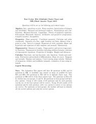
1121.61.41.51.2110.80.60.50.40.201.500.810.50.20 01(a)0.40.60.810.60.40.2001(b)0.20.40.60.87186.5166145.554.54121083.56342.51210.80.60.40.20.20 02(a)0.40.60.810.80.60.40.2000.22(b)0.40.60.81Fig. 9.The final non-dominated front obtained by (a) AMOSA (b) MOSA for the test problems (1) DTLZ5 (2) DTLZ6be seen from this table that AMOSA performs the best interms of Purity and Convergence for DTLZ1, DTLZ3, DTLZ5,DTLZ6. In DTLZ2 and DTLZ4 the performance of MOSA ismarginally better than that of AMOSA. NSGA-II performs theworst among all. Table V shows the Minimal Spacing valuesobtained by the 3 algorithms for DTLZ1-DTLZ6. AMOSAperforms the best in all the cases.As mentioned earlier, for comparing the performance ofMOSA (by considering the results reported in [32]), a versionof AMOSA without clustering and with unconstrained archiveis executed. The results reported here are the average over 10runs. Table VI shows the corresponding Purity, Convergenceand Minimal Spacing values. Again AMOSA performs muchbetter than MOSA for all the test problems except DTLZ4. ForDTLZ4, the MOSA performs better than that of AMOSA interms of both Purity and Convergence values. Figure 8 showsfinal Pareto-optimal front obtained by AMOSA and MOSAfor DTLZ1-DTLZ3 while Figure 9 shows the same for DTLZ5and DTLZ6. As can be seen from the figures, AMOSA appearsto be able to better approximate the front with more densesolutions as compared to MOSA.It was mentioned in [33] that for a particular test problem,almost 40% of the solutions provided by an algorithm withtruncation of archive got dominated by the solutions providedby an algorithm without archive truncation. However theexperiments we conducted did not adequately justify thisfinding. Let us denote the set of solutions of AMOSA withand without clustering as S c and S wc respectively. We foundthat for DTLZ1, 12.6% of S c were dominated by S wc , while4% of S wc were dominated by S c . For DTLZ2, 5.1% of S wcwere dominated by S c while 5.4% of S c were dominated byS wc . For DTLZ3, 22.38% of S wc were dominated by S c while0.53% of S c were dominated by S wc . For DTLZ4, all themembers of S wc and S c are non-dominating to each otherand the solutions are same. Because execution of AMOSAwithout clustering doesn’t provide more than 100 solutions.For DTLZ5, 10.4% of S wc were dominated by S c while 0.5%of S c were dominated by S wc . For DTLZ6, all the membersof S wc and S c are non-dominating to each other.To have a look at the performance of the AMOSA on afour-objective problem, we apply AMOSA and NSGA-II tothe 13-variable DTLZ2 test problem. This is referred to asDTLZ2 4. The problem has a spherical Pareto-front in fourdimensions given by the equation: f1 2 +f2 2 +f2 3 +f2 4 = 1 withf i ∈ [0, 1] for i = 1 to 4. Both the algorithms are applied for atotal of 30,000 function evaluations (for NSGA-II popsize=100and number of generations=300) and the Purity, Convergenceand Minimal Spacing values are shown in Table VII. AMOSAperforms much better than NSGA-II in terms of all the threemeasures.The proposed AMOSA and NSGA-II are also comparedfor DTLZ1 5 (9-variable 5 objective version of the test problemDTLZ1), DTLZ1 10 (14-variable 10 objective versionof DTLZ1) and DTLZ1 15 (19 variable 15 objective versionof DTLZ1). The three problems have a spherical Paretofrontin their respective dimensions given by the equation∑ Mi=1 f i = 0.5 where M is the total number of objectivefunctions. Both the algorithms are executed for a total of1,00,000 function evaluations for these three test problems(for NSGA-II popsize=200, number of generations=500) andthe corresponding Purity, Convergence and Minimal Spacingvalues are shown in Table VII. Convergence value indicatesthat NSGA-II doesn’t converge to the true PO front whereas AMOSA reaches the true PO front for all the three cases.

12TABLE VConvergence AND Purity MEASURES ON THE 3 OBJECTIVE TEST FUNCTIONS WHILE Archive IS BOUNDED TO 100Test Convergence P urity MinimalSpacingProblem AMOSA MOSA NSGA-II AMOSA MOSA NSGA-II AMOSA MOSA NSGA-IIDT LZ1 0.01235 0.159 13.695 0.857 0.56 0.378 0.0107 0.1529 0.2119(85.7/100) (28.35/75) (55.7/100)DT LZ2 0.014 0.01215 0.165 0.937 0.9637 0.23 0.0969 0.1069 0.1236(93.37/100) (96.37/100) (23.25/100)DT LZ3 0.0167 0.71 20.19 0.98 0.84 0.232 0.1015 0.152 0.14084(93/95) (84.99/100) (23.2/70.6)DT LZ4 0.28 0.21 0.45 0.833 0.97 0.7 0.20 0.242 0.318(60/72) (97/100) (70/100)DT LZ5 0.00044 0.0044 0.1036 1 0.638 0.05 0.0159 0.0579 0.128(97/97) (53.37/83.6) (5/100)DT LZ6 0.043 0.3722 0.329 0.9212 0.7175 0.505 0.1148 0.127 0.1266(92.12/100) (71.75/100) (50.5/100)TABLE VIConvergence, Purity AND Minimal Spacing MEASURES ON THE 3 OBJECTIVES TEST FUNCTIONS BY AMOSA AND MOSA WHILE Archive IS UNBOUNDEDTest Convergence P urity MinimalSpacingProblem AMOSA MOSA AMOSA MOSA AMOSA MOSADT LZ1 0.010 0.1275 0.99(1253.87/1262.62) 0.189(54.87/289.62) 0.064 0.083.84DT LZ2 0.0073 0.0089 0.96(1074.8/1116.3) 0.94(225/239.2) 0.07598 0.09595DT LZ3 0.013 0.025 0.858(1212/1412.8) 0.81(1719/2003.9) 0.0399 0.05DT LZ4 0.032 0.024 0.8845(88.5/100) 0.4050(38.5/94.9) 0.1536 0.089DT LZ5 0.0025 0.0047 0.92(298/323.66) 0.684(58.5/85.5) 0.018 0.05826DT LZ6 0.0403 0.208 0.9979(738.25/739.75) 0.287(55.75/194.25) 0.0465 0.0111TABLE VIIConvergence, Purity AND Minimal Spacing MEASURES ON THE DTLZ2 4, DTLZ1 5, DTLZ1 10 AND DTLZ1 15 TEST FUNCTIONS BY AMOSA ANDNSGA-IITest Convergence P urity MinimalSpacingProblem AMOSA NSGA-II AMOSA NSGA-II AMOSA NSGA-IIDT LZ2 4 0.2982 0.4563 0.9875(98.75/100) 0.903(90.3/100) 0.1876 0.22DT LZ1 5 0.0234 306.917 1 0 0.1078 0.165DT LZ1 10 0.0779 355.957 1 0 0.1056 0.2616DT LZ1 15 0.193 357.77 1 0 0.1 0.271The Purity measure also indicates this. The results on manyobjectiveoptimization problems show that AMOSA peformsmuch better than NSGA-II. These results support the fact thatPareto ranking-based MOEAs such as NSGA-II do not workwell on many-objective optimization problems as pointed outin some recent studies [26], [27].D. Discussion on Annealing ScheduleThe annealing schedule of an SA algorithm consists of (i)initial value of temperature (T max), (ii) cooling schedule, (iii)number of iterations to be performed at each temperature and(iv) stopping criterion to terminate the algorithm. Initial valueof the temperature should be so chosen that it allows the SAto perform a random walk over the landscape. Some methodsto select the initial temperature are given in detail in [18]. Inthis article, as in [17], we have set the initial temperature toachieve an initial acceptance rate of approximately 50% onderogatory proposals. This is described in Section VI.C.Cooling schedule determines the functional form of thechange in temperature required in SA. The most frequentlyused decrement rule, also used in this article, is the geometricschedule given by: T k+1 = α × T k , where α (0 < α

13poorer. However, an exhaustive sensitivity study needs to beperformed for AMOSA.The third component of an annealing schedule is the numberof iterations performed at each temperature. It should be sochosen that the system is sufficiently close to the stationarydistribution at that temperature. As suggested in [18], the valueof the number of iterations should be chosen depending onthe nature of the problem. Several criteria for termination ofan SA process have been developed. In some of them, thetotal number of iterations that the SA procedure must executeis given, where as in some other, the minimum value of thetemperature is specified. Detailed discussion on this issue canbe found in [18].V. DISCUSSION AND CONCLUSIONSIn this article a simulated annealing based multi-objectiveoptimization algorithm has been proposed. The concept ofamount of domination is used in solving the multi-objectiveoptimization problems. In contrast to most other MOO algorithms,AMOSA selects dominated solutions with a probabilitythat is dependent on the amount of domination measuredin terms of the hypervolume between the two solutions inthe objective space. The results of binary-coded AMOSAare compared with those of two existing well-known multiobjectiveoptimization algorithms - NSGA-II (binary-coded)[19] and PAES [20] for a suite of seven 2-objective testproblems having different complexity levels. In a part of theinvestigation, comparison of the real-coded version of theproposed algorithm is conducted with a very recent multiobjectivesimulated annealing algorithm MOSA [17] and realcodedNSGA-II for six 3-objective test problems. Real-codedAMOSA is also compared with real-coded NSGA-II for some4, 5, 10 and 15 objective test problems. Several different comparisonmeasures like Convergence, Purity, MinimalSpacing,and Spacing, and the time taken are used for the purposeof comparison. In this regard, a measure called displacementhas also been used that is able to reflect whether a front isclose to the PO front as well as its extent of coverage. Acomplexity analysis of AMOSA is performed. It is found thatits complexity is more than that of PAES but smaller than thatof NSGA-II.It is seen from the given results that the performance of theproposed AMOSA is better than that of MOSA and NSGA-IIin a majority of the cases, while PAES performs poorly ingeneral. AMOSA is found to provide more distinct solutionsthan NSGA-II in each run for all the problems; this is a desirablefeature in MOO. AMOSA is less time consuming thanNSGA-II for complex problems like ZDT1, ZDT2 and ZDT6.Moreover, for problems with many objectives, the performanceof AMOSA is found to be much better than that of NSGA-II. This is an interesting and appealing feature of AMOSAsince Pareto ranking-based MOEAs, such as NSGA-II [19]do not work well on many-objective optimization problems aspointed out in some recent studies [26], [27]. An interestingfeature of AMOSA, as in other versions of multi-objective SAalgorithms, is that it has a non-zero probability of allowinga dominated solution to be chosen as the current solutionin favour of a dominating solution. This makes the problemless greedy in nature; thereby leading to better performancefor complex and/or deceptive problems. Note that it may bepossible to incorporate this feature as well as the concept ofamount of domination in other MOO algorithms in order toimprove the performance.There are several ways in which the proposed AMOSAalgorithm may be extended in future. The main time consumingprocedure in AMOSA is the clustering part. Someother more efficient clustering techniques or even the PAESlike grid based strategy, can be incorporated for improving itsperformance. Implementation of AMOSA with unconstrainedarchive is another interesting area to pursue in future. Analgorithm, unless analyzed theoretically, is good for only theexperiments conducted. Thus a theoretical analysis of AMOSAneeds to be performed in the future in order to study itsconvergence properties. Authors are currently trying to developa proof for the convergence of AMOSA in the lines of theproof for single objective SA given by Geman and Geman [4].As has been mentioned in [18], there are no firm guidelinesfor choosing the parameters in an SA-based algorithm. Thus,an extensive sensitivity study of AMOSA with respect to itsdifferent parameters, notably the annealing schedule, needs tobe performed. Finally, application of AMOSA to several reallifedomains e.g., VLSI system design [34], remote sensingimagery [35], data mining and Bioinformatics [36], needs tobe demonstrated. The authors are currently working in thisdirection.REFERENCES[1] K. Deb, Multi-objective Optimization Using Evolutionary Algorithms.England: John Wiley and Sons, Ltd, 2001.[2] C. Coello, D. V. Veldhuizen, and G. Lamont, Evolutionary Algorithmsfor Solving Multi-Objective Problems. Boston: Kluwer AcademicPublishers, 2002.[3] S. Kirkpatrick, C. Gelatt, and M. Vecchi, “Optimization by simulatedannealing,” Science, vol. 220, pp. 671–680, 1983.[4] S. Geman and D. Geman, “Stochastic relaxation, Gibbs distributionsand the Bayesian restoration of images,” IEEE-Transactions on PatternAnalysis and Machine Intelligence, vol. 6, no. 6, pp. 721–741, 1984.[5] S. Bandyopadhyay, U. Maulik, and M. K. Pakhira, “Clustering usingsimulated annealing with probabilistic redistribution,” InternationalJournal of Pattern Recognition and Artificial Intelligence, vol. 15, no. 2,pp. 269–285, 2001.[6] R. Caves, S. Quegan, and R. White, “Quantitative comparison of theperformance of SAR segmentation algorithms,” IEEE Transactions onImage Proc., vol. 7, no. 11, pp. 1534–1546, 1998.[7] U. Maulik, S. Bandyopadhyay, and J. Trinder, “SAFE: An efficientfeature extraction technique,” Journal of Knowledge and InformationSystems, vol. 3, pp. 374–387, 2001.[8] P. Czyzak and A. Jaszkiewicz, “Pareto simulated annealing - a metaheuristictechnique for multiple-objective combinatorial optimization,”Journal of Multi-Criteria Decision Analysis, vol. 7, pp. 34–47, 1998.[9] M. Hapke, A. Jaszkiewicz, and R. Slowinski, “Pareto simulated annealingfor fuzzy multi-objective combinatorial optimization,” Journal ofHeuristics, vol. 6, no. 3, pp. 329–345, 2000.[10] A. Suppapitnarm, K. A. Seffen, G. T. Parks, and P. Clarkson, “A simulatedannealing algorithm for multiobjective optimization,” EngineeringOptimization, vol. 33, pp. 59–85, 2000.[11] D. K. Nam and C. Park, “Multiobjective simulated annealing: a comparativestudy to evolutionary algorithms,” Int. J. Fuzzy Systems, vol. 2,no. 2, pp. 87–97, 2000.[12] E. L. Ulungu, J. Teghaem, P. Fortemps, and D. Tuyttens, “MOSAmethod: a tool for solving multiobjective combinatorial decision problems,”J. multi-criteria decision analysis, vol. 8, pp. 221–236, 1999.

14[13] D. Tuyttens, J. Teghem, and N.El-Sherbeny, “A particular multiobjectivevehicle routing problem solved by simulated annealing,” Metaheuristicsfor multiobjective optimization, vol. 535, pp. 133–152, 2003.[14] I. Das and J. Dennis, “A closer look at drawbacks of minimizingweighted sums of objectives for pareto set generation in multicriteriaoptimization problems,” Structural Optimization, vol. 14, no. 1, pp. 63–69, 1997.[15] A. Jaszkiewicz, “Comparison of local search-based metaheuristics onthe multiple objective knapsack problem,” Foundations of computer anddecision sciences, vol. 26, no. 1, pp. 99–120, 2001.[16] B. Suman, “Study of self-stopping PDMOSA and performance measurein multiobjective optimization,” Computers and Chemical Engineering,vol. 29, no. 5, pp. 1131–1147, 15 April 2005.[17] K. Smith, R. Everson, and J. Fieldsend, “Dominance measures formulti-objective simulated annealing,” in Proceedings of the 2004 IEEECongress on Evolutionary Computation (CEC’04), 2004, pp. 23–30.[18] B. Suman and P. Kumar, “A survey of simulated annealing as a toolfor single and multiobjective optimization,” Journal of the OperationalResearch Society, vol. 57, no. 10, pp. 1143–1160, 2006.[19] K. Deb, A. Pratap, S. Agarwal, and T. Meyarivan, “A fast and elitistmultiobjective genetic algorithm: NSGA-II,” IEEE Transactions onEvolutionary Computation, vol. 6, no. 2, 2002.[20] J. D. Knowles and D. W. Corne, “Approxmating the nondominated frontusing the pareto archived evolution strategy,” Evolutionary Computation,vol. 8, no. 2, pp. 149–172, 2000.[21] S. Bandyopadhyay, S. K. Pal, and B. Aruna, “Multi-objective GAs,quantitative indices and pattern classification,” IEEE Transactions onSystems, Man and Cybernetics-B, vol. 34, no. 5, pp. 2088–2099, 2004.[22] H. Ishibuchi and T. Murata, “A multi-objective genetic local search algorithmand its application to flowshop scheduling,” IEEE Transactionson Systems, Man and Cybernetics-Part C: Applications and Reviews,vol. 28, no. 3, pp. 392–403, August, 1998.[23] J. R. Schott, “Fault tolerant design using single and multi-criteria geneticalgorithms,” Ph.D. dissertation, 1995.[24] H. Ishibuchi, T. Yoshida, and T. Murata, “Balance between geneticserach and local serach in memetic algorithms for multiobjectivepermutation flowshop scheduling,” IEEE-Transactions on EvolutionaryComputation, vol. 6, no. 6, pp. 721–741, 1984.[25] E. Zitzler and L. Thiele, “An evolutionary algorithm for multiobjectiveoptimization: The strength pareto approach,” Gloriastrasse 35, CH-8092Zurich, Switzerland, Tech. Rep. 43, 1998.[26] E. J. Hughes, “Evolutionary many-objective optimization: Many onceor one many?” in Proceedings of 2005 Congress on EvolutionaryComputation, Edinburgh, Scotland, UK, September 2-5, 2005, pp. 222–227.[27] H. Ishibuchi, T. Doi, and Y. Nojima, “Incorporation of scalarizing fitnessfunctions into evolutionary multiobjective optimization algorithms,” InParallel Problem Solving from Nature IX ( PPSN-IX), vol. 4193, pp.493–502, September 2006.[28] J. Fieldsend, R. Everson, and S. Singh, “Using unconstrained elitearchives for multi-objective optimisation,” IEEE Transactions on EvolutionaryComputation, vol. 7, no. 3, pp. 305–323, 2003.[29] A. K. Jain and R. C. Dubes, Algorithms for Clustering Data. EnglewoodCliffs, NJ: Prentice-Hall, 1988.[30] G. Toussaint, “Pattern recognition and geometrical complexity,” inProc. Fifth International Conf. on Pattern Recognition, Miami Beach,December 1980, pp. 1324–1347.[31] K. Deb, “Multi-objective genetic algorithms: problem difficulties andconstruction of test problems,” Evolutionary Computation, vol. 7, no. 3,pp. 205–230, 1999.[32] http://www.dcs.ex.ac.uk/people/kismith/mosa/results/tec/.[33] E. Zitzler, K. Deb, and L. Thiele, “Comparison of multiobjectiveevolutionary algorithms: Empirical results,” Evolutionary Computation,vol. 8, no. 2, pp. 173–195, 2000.[34] S. Saha, S.Sur-Kolay, S. Bandyopadhyay, and P. Dasgupta, “Multiobjectivegenetic algorithm for k-way equipartitioning of a point setwith application to CAD-VLSI,” in Proceedings of 9th InternationalConference on Information Technology (ICIT 2006). IEEE ComputerSociety, December, 2006, pp. 281–284.[35] S. Bandyopadhyay, U. Maulik, and A. Mukhopadhyay, “Multiobjectivegenetic clustering for pixel classification in remote sensing imagery,”IEEE Transactions Geoscience and Remote Sensing (In Press), 2006.[36] A. Mukhopadhyay, U. Maulik, and S. Bandyopadhyay, “Efficient twostagefuzzy clustering of microarray gene expression data,” in Proceedingsof 9th International Conference on Information Technology (ICIT2006). IEEE Computer Society, December, 2006, pp. 11–14.Sanghamitra Bandyopadhyay (SM’05) did herBachelors in Physics and Computer Science in 1988and 1991 respectively. Subsequently, she did herMasters in Computer Science from Indian Instituteof Technology (IIT), Kharagpur in 1993 and Ph.D inComputer Science from Indian Statistical Institute,Calcutta in 1998. Currently she is an AssociateProfessor, Indian Statistical Institute, Kolkata, India.Dr. Bandyopadhyay is the first recipient of DrShanker Dayal Sharma Gold Medal and InstituteSilver Medal for being adjudged the best all roundpost graduate performer in IIT, Kharagpur in 1994. She has worked in LosAlamos National Laboratory, Los Alamos, USA, in 1997, University of NewSouth Wales, Sydney, Australia, in 1999, Department of Computer Scienceand Engineering, University of Texas at Arlington, USA, in 2001, Universityof Maryland, Baltimore County, USA, in 2004, Fraunhofer Institute AiS, St.Augustin, Germany, in 2005 and Tsinghua University, China, in 2006. Shehas delivered lectures at Imperial College, London, UK, Monash University,Australia, University of Aizu, Japan, University of Nice, France, UniversityKebangsaan Malaysia, Kuala Lumpur, Malaysia, and also made academicvisits to many more Institutes/Universities around the world. She is a co-authorof 3 books and more than 100 research publications. Dr. Bandyopadhyayreceived the Indian National Science Academy (INSA) and the Indian ScienceCongress Association (ISCA) Young Scientist Awards in 2000, as well as theIndian National Academy of Engineering (INAE) Young Engineers’ Awardin 2002. She has guest edited several journal special issues including IEEETransactions on Systems, Man and Cybernetics, Part - B. Dr. Bandyopadhyayhas been the Program Chair, Tutorial Chair, Associate Track Chair and aMember of the program committee of many international conferences. Herresearch interests include Pattern Recognition, Data Mining, Evolutionary andSoft Computation, Bioinformatics and Parallel and Distributed Systems.Sriparna Saha received her B.Tech degree in ComputerScience and Engineering from Kalyani Govt.Engineering College, University of Kalyani, Indiain 2003. She did her M.Tech in Computer Sciencefrom Indian Statistical Institute, Kolkata in 2005.She is the recipient of Lt Rashi Roy Memorial GoldMedal from Indian Statistical Institute for outstandingperformance in M.Tech (Computer Science). Atpresent she is pursuing her Ph.D. from Indian StatisticalInstitute, Kolkata, India. She is a co-authorof about 10 papers. Her research interests includeMultiobjective Optimization, Pattern Recognition, Evolutionary Algorithms,and Data Mining.Ujjwal Maulik (SM’05) is currently a Professor inthe Department of Computer Science and Engineering,Jadavpur University, Kolkata, India. Dr. Maulikdid his Bachelors in Physics and Computer Sciencein 1986 and 1989 respectively. Subsequently, he didhis Masters and Ph.D in Computer Science in 1991and 1997 respectively. He was the Head of the schoolof Computer Science and Technology Department ofKalyani Govt. Engg. College, Kalyani, India during1996-1999. Dr. Maulik has worked in Center forAdaptive Systems Application, Los Alamos, NewMexico, USA in 1997, University of New South Wales, Sydney, Australiain 1999, University of Texas at Arlington, USA in 2001, Univ. of MarylandBaltimore County, USA in 2004 and Fraunhofer Institute AiS, St. Augustin,Germany in 2005. He has also visited many Institutes/Universities around theworld for invited lectures and collaborative research. He is a senior memberof IEEE and a Fellow of IETE, India. Dr. Maulik is a co-author of 2 booksand about 100 research publications. He is the recipient of the Govt. of IndiaBOYSCAST fellowship in 2001. Dr. Maulik has been the Program Chair,Tutorial Chair and a Member of the program committee of many internationalconferences and workshops. His research interests include Artificial Intelligenceand Combinatorial Optimization, Soft Computing, Pattern Recognition,Data Mining, Bioinformatics, VLSI and Distributed System.

Kalyanmoy Deb is currently a Professor of MechanicalEngineering at Indian Institute of TechnologyKanpur, India and is the director of Kanpur GeneticAlgorithms Laboratory (KanGAL). He is therecipient of the prestigious Shanti Swarup BhatnagarPrize in Engineering Sciences for the year 2005. Hehas also received the ‘Thomson Citation LaureateAward’ from Thompson Scientific for having highestnumber of citations in Computer Science during thepast ten years in India. He is a fellow of IndianNational Academy of Engineering (INAE), IndianNational Academy of Sciences, and International Society of Genetic andEvolutionary Computation (ISGEC). He has received Fredrick Wilhelm BesselResearch award from Alexander von Humboldt Foundation in 2003. His mainresearch interests are in the area of computational optimization, modelingand design, and evolutionary algorithms. He has written two text books onoptimization and more than 190 international journal and conference researchpapers. He has pioneered and a leader in the field of evolutionary multiobjectiveoptimization. He is associate editor of two major international journalsand an editorial board members of five major journals. More informationabout his research can be found from http://www.iitk.ac.in/kangal/deb.htm.15