Solving the time dependent Schrodinger equation

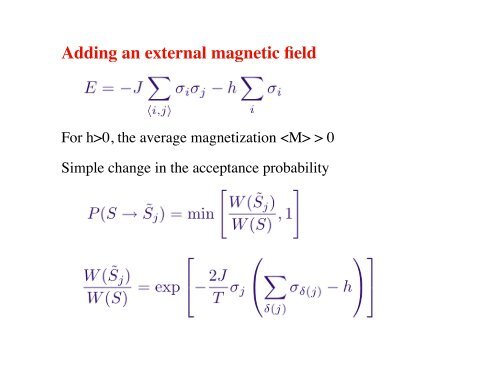
Adding an external magnetic field For h>0, the average magnetization > 0 Simple change in the acceptance probability

Elements of a simulation program Module with: • system dimensions; n=l*l• pregenerated acceptance probabilities; pflip(-4:4)• spin array; spin(0:n-1)module systemvariablesimplicit noneinteger :: linteger :: nreal :: pflip(-4:4)integer, allocatable :: spin(:)end module systemvariables

Main program open(1,file='ising.in',status='old')read(1,*)lread(1,*)tempread(1,*)binsread(1,*)binstepsclose(1)call initialize(temp)do i=1,binstepscall mcstependdodo j=1,binscall resetdatasumsdo i=1,binstepscall mcstepcall measureenddocall writebindata(n,binsteps)enddo

Initialization tasks subroutine initialize(temp)use systemvariablesn=l*ldo i=-4,4,2pflip(i)=exp(-i*2./temp)enddocall random_seed(put=seed)allocate(spin(0:n-1))do i=0,n-1call random_number(r)spin(i)=2*int(2.*r)-1enddohere I-sum corresponds to jnumber spins i=0,…,n-1 No field (h=0). Small Modification for h>0 (see program on-line)jj

Performs one Monte Carlo step subroutine mcstep() do i=1,ncall random_number(r)s=int(r*n)spins are labeled s=0,…,n-1x=mod(s,l); y=s/ls1=spin(mod(x+1,l)+y*l)s2=spin(mod(x-1+l,l)+y*l)s3=spin(x+mod(y+1,l)*l)s4=spin(x+mod(y-1+l,l)*l)call random_number(r)if (r

Measures observables (energy, magnetization, and their squares) subroutine measurereal(8) :: enrg1,enrg2,magn1,magn2common/measurments/enrg1,enrg2,magn1,magn2 e=0; m=0do s=0,n-1x=mod(s,l); y=s/le=e-spin(s)*(spin(mod(x+1,l)+y*l))e=e-spin(s)*(spin(x+mod(y+1,l)*l))enddom=sum(spin)enrg1=enrg1+dble(e)enrg2=enrg2+dble(e)**2magn1=magn1+abs(m)magn2=magn2+dble(m)**2

Writes bin averages to a file subroutine writebindata(n,steps)real(8) :: enrg1,enrg2,magn1,magn2common/measurments/enrg1,enrg2,magn1,magn2open(1,file='bindata.dat',position='append')enrg1=enrg1/(dble(steps)*dble(n))enrg2=enrg2/(dble(steps)*dble(n)**2)magn1=magn1/(dble(steps)*dble(n))magn2=magn2/(dble(steps)*dble(n)**2)write(1,1)enrg1,enrg2,magn1,magn21 format(4f18.12)close(1)These bin data should be processed (giving final averages and statistical errors) with a separate program.

Squared magnetization for different system sizes (no external field): development of phase transition

Finite-size scaling T > T c : → 0 (exponentially) T = T c : → 0 (power law) T < T c : → constant > 0 Extracting an exponent: - Power-law: straight line when plotted on log-log scale