Demonstration Applets for Introductory Statistics

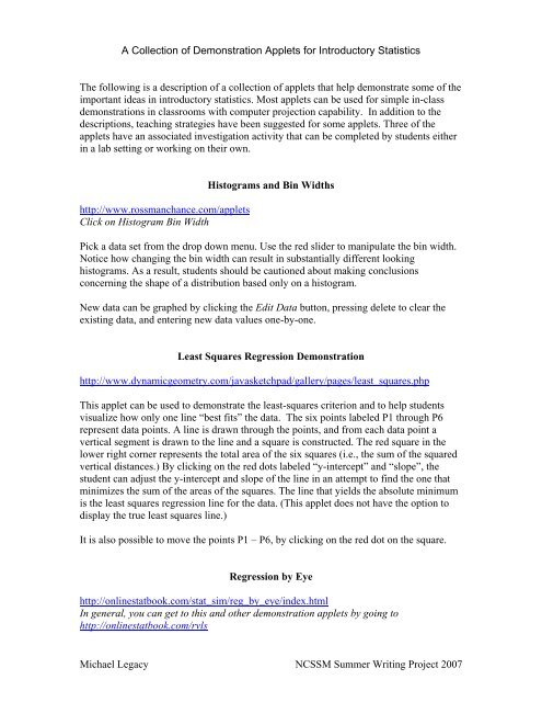
Using a Normal Approximation for the Binomial Distributionhttp://www.whfreeman.com/tps3eClick on Statistical Applets and then Central Limit Theorem Normal Approximation toBinomial DistributionsAs n increases, the binomial distribution with n trials and probability of success p can bebetter and better approximated by a normal distribution. This applet uses sliders tochange both n and p. You can click and drag a slider with the mouse.The histogram shows the binomial probabilities. The vertical black line marks the mean µ= np. The red curve is the normal density curve with the same mean and standarddeviation as the B(n,p) distribution ( µ = np and σ = np(1 − p)). Use the slider to setlower and higher values of p.Teaching strategy: Let students investigate various values for n and p. What values of nand p seem to yield a binomial distribution that can be reasonably approximated by anormal distribution? Students should note that the binomial probability distributionbecomes more skewed as p moves farther away from 0.5. In order for the binomialprobability histogram to look more like a normal curve, students should discover the needto increase n as p becomes more extreme.This activity helps explain why the conditions check on large sample size for inferenceon proportions involves verifying that np > 10 and n(1 − p) > 10 . Note that some bookssuggest checking against 5 or 15.Investigating Sampling DistributionsThis investigation directs students to explore various aspects of sampling distributionsusing the Rice Virtual Lab in Statistics simulation at www.onlinestatbook.com/rvls. Seeactivity titled Investigations of sample statistic distributions using an on-line simulator.Investigating a Sampling Distribution of Sample Proportionshttp://www.rossmanchance.com/applets. Click on Reeses PiecesThis applet lets you build a sampling distribution of sample proportions using ReesesPieces. The parameterθ represents the proportion of orange candies in the population inthe candy machine. To start, set θ =.6, a sample size of n = 10 , and the num samples tobe drawn at 1. Click the Animate box and then click the Draw Samples button. Tencandies will fall from the machine into the bins below sorted by color. The red ˆp is theproportion of the sample that is orange. The proportion of orange candies in the sample isMichael Legacy NCSSM Summer Writing Project 2007

also shown on the dotplot. Click Draw Samples a few more times to begin building thesampling distribution of sample proportions. (The use of the Animate button does slowthis procedure down for students to actually see the process of building the distribution.)Change the num samples to 10 and click Draw Samples. Once students are clear on theprocess, deselect the Animate button and change num samples to 50. Also select the plotnormal curve box. Click Draw Samples several times. How closely is the samplingdistribution of sample proportions approximated by the normal curve?Teaching Strategy: Vary the investigation with different values of n andθ . Click Reseteach time you want to clear the sampling distribution dotplot. Have students determinewhat values of n and θ yield a sampling distribution that is approximately normal.Understanding Confidence Levelhttp://www.whfreeman.com/tps3eClick on Statistical Applets and then Confidence IntervalNote: It is important that students understand the concept of a sampling distributionbefore introducing them to confidence intervals. Good activities for understandingsampling distributions are the two previous investigations.This applet can be used to develop a basic understanding of a confidence level forconstructing a confidence interval to estimate the mean (µ) of a population. Set thedesired confidence level by clicking on the radio buttons to the left of the plot. Start with80%. Click the Sample button for a single SRS. Do this a few times. Each clickrepresents drawing one sample. The dot marks the sample mean, which is the center ofthe interval. The lines on each side of the dot span the confidence interval. Emphasizethat each sample drawn from the population results in an x for that sample along with aninterval estimate of the population mean µ and that a different sample will yield adifferent estimate of µ .Note that once in a while an interval “misses” the mean (µ). This miss will show up inRed. The accumulator on the right hand side will record the total number of samplesdrawn and the number of times the interval correctly contains the population mean µ.Click the Sample 50 button. Do this enough times to accumulate a few hundred samples.Note that the percent of “hits” will hover around 80%. For this example, on average, inrepeated sampling, 80% of the samples drawn will yield an interval that correctlyestimates the mean of the population. Caution: Students are tempted to phrase this as aprobability. Not so! The probability that you have a correct estimate is either 0 or 1 (youhave correctly estimated µ or you have not.) Since µ is unknown, there is no way ofknowing for sure. That is why it is expressed as a confidence in the estimate.Have students conjecture about the effect of increasing the confidence level to 90%, 95%,and 99%. Will the true mean be captured more often, less often, or will the frequencyremain the same? Using the same screen you currently have, click through the radiobuttons, increasing the confidence level as you go to observe how the lengths of theMichael Legacy NCSSM Summer Writing Project 2007

confidence intervals change. Have students work though the previous exercise usingdifferent confidence levels.Investigating Errors and Power in Significance Tests for Means (σ is known)Starting with a problem situation about a packaging machine, students simulate theprobability of committing Type I and II errors by using a power applet athttp://wise.cgu.edu/power_applet.asp. In addition, students investigate the power of a testby changing the α -value, the sample size, and the difference between the hypothesizedmean and the true mean. See the activity Investigating Errors and Power in SignificanceTests for Means (σ is known).Sampling Regression Lines ActivityThis investigation lets students examine the sampling distribution of sample slopes for alinear regression. The applet allows the student to first look at possible sample slopes oneat a time. The student then draws 100 samples to examine the sampling distribution ofsample slopes. The student varies sample size, the population standard deviationσ , andthe spread of the x-values, to determine their effect on the variability of the sampleslopes. See the activity Sampling Regression Lines Using an On-Line Simulation.Michael Legacy NCSSM Summer Writing Project 2007