GEOLOGICAL MODELING AND SIMULATION OF CO2 ... - Sintef

2 EIGESTAD, DAHLE, HELLEVANG, RIIS, JOHANSEN, AND ØIANaccess from the Troll field, promising geological properties and sealing propertiesshown by initial modeling, and proximity to Mongstad. The Johansenformation therefore appears to be an excellent candidate for storage of CO 2from Kårstø and particularly the Mongstad power plant. Early case studies [9]have also shown pipeline solutions to outperform combined wessel/pipeline solutionsin terms of economical viability, and a long term pipeline solution fromMongstad may be feasible.The estimation of the storage capacity of deep saline aquifers is very complexsince various trapping mechanisms are involved and act on different time scales[4],[5],[7],[15], [26]. Geological uncertainty and/or lack of geological characterizationadd further to this complexity. In the end, conservative estimates ofthe amount of CO 2 that escape the boundaries of an aquifer within a giventime frame, and the consequences of leakage must be provided. Because ofcomputational limitations and lack of information which require a stochasticframework, new modeling tools need to be developed to perform this type ofanalysis. Such modeling tools have been proposed and are developed by Celiaand Nordbotten with collaborators in the context of mature sedimentary basinsin the North America, see [18], [19], [20], [21], [22]. Their focuses have been tohandle large numbers of abandoned and potentially leaky wells within simplelayered geometry which allows for semi-analytic solutions. North Sea aquifersmay on the on the other hand provide different challenges, including complexgeometries and fault/fracture zones which may provide pathways for leakage.To understand the main effects that should be accounted for in capacity/riskanalysis, detailed simulations must be performed using verified simulation toolsas a first step.The purpose of this work is two-folded: First we wish to provide a backgroundto the benchmark 3 problem presented at the Workshop on Numerical Modelsfor Carbon Dioxide Storage in Geological Formations, Stuttgart April 2-4, 2008,[8]. This was a benchmark study based on the geological data for the Johansenformation, but on a simplified geometry and a small extract of the entire model.The workshop demonstrated that different modeling groups need to communicateto calibrate and understand the workings of computational tools, but alsothe need for real data to be provided for the modeling community. The geologicalmodel presented in this work is therefore made available online, see [11],and a complete dataset is made available for simple CO 2 flow. Secondly, we investigatesome of the factors that we believe are important in obtaining reliablecapacity estimates of a formation, using the commercial simulator Eclipse 100[12]. The numerical simulations presented here may be used for comparisonsof simulations, and a motivation for more advanced studies. Probably one ofthe most important factors is to determine appropriate boundary conditions forthe formation. We show that different choices of boundary conditions stronglyaffect the time variation of the pressure field and the CO 2 plume distribution.A major numerical concern is the need for grid resolution. We show that afairly fine vertical resolution is needed to capture the CO 2 plume that followsthe sealed roof of the formation due to gravity override. Moreover, vertical gridrefinement of the sealing shale layer is needed because of upstream weighting inthe numerical simulation tool. The upstream weighting without grid refinement

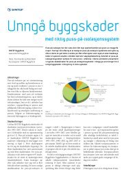
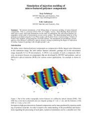
leads to numerical diffusion which may appear as leakage into the formationsabove. Consequently, the numerical resolution may need to be higher than inthe original geological grid. We then simulate post injection migration to investigatethe potential effect of residual trapping and relative permeability models.The geometry and topology of the geological medium will also play a key partfor CO 2 distribution. Finally, we investigate the sensitivity of the plume distributionwith respect to permeability models. Dissolution and mineral trappingmechanisms [4],[5] are not considered in this work and are typically importantover longer time-scales than the simulation studies performed here.The rest of the paper is organised as follows: Section 2 provides an overview,and discusses geological modeling of the formation. Section 3 gives more detailsof the data which is made available, and discusses simulation issues and set-up.Section 4 presents some simulation results for injection of CO 2 in the Johansenformation. Conclusions are given in Section 5.32. Overview of the Johansen formation and geological modelingThe Johansen formation is located in the deeper part of the Sognefjord delta,60 km offshore the Mongstad area at the west coast of Norway. The Troll fieldis situated some 500 meters above the north-western parts of the Johansen formation,and is one of the largest gas fields in the North Sea. The SognefjordFormation which is situated more than 500 meters above the Johansen Formation,is the uppermost sand in the Sognefjord delta. The Sognefjord Formationis the main reservoir for the giant Troll gas and oil field. Figure 1 shows thegeographic locations of various fields and sites of interest together with partsof the south-western coast of Norway. The two red dots indicate the locationthe planned power plants at Kårstø and Mongstad. The depth levels of theJohansen formation range from 2200-3100 m below sea level, which makes theformation ideal for CO 2 storage due to the pressure regimes that exist here.The average thickness of the formation is roughly 100 m and the lateral extensionsare up to 100 km in the north-south direction and 60 km in the east-westdirection. With average porosities of approximately 25 percent this implies thatthe theoretical storage capacity of the Johansen formation is of the order > 1Gt CO 2 when also accounting for residual brine saturation (approximately 20percent).Figure 2 shows a cross-section from the geological model in the southernpart of the proposed injection area. Mainly sandy layers are shown by yellowcolours, and shaly layers with grey and black. The Troll Field is located above1550 m depth north and east of the section (red colour). The model is based onmapping of the existing seismic and well data, including high quality 3D seismicdata sets in the area of the Troll Field, and a 2D seismic grid of fair quality fromthe 1990’ies south of the field. We have used log data from 12 exploration wellsin the Troll Field and a few additional wells from neighbouring fields which havepenetrated the Johansen Formation or its equivalents. One of the wells has ashort core in the Johansen Formation. The purpose of the model was to serve asa basis for a quick evaluation of the feasibility of using the Johansen formationfor CO2 sequestration. Consequently, the model represents a simplification of

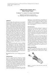
5Figure 2. Geological model of area that is being investigated forCO 2 storage in the Johansen formation. Topographical surface showstop of sandstone reservoir where the Troll gas is located. Troll fieldindicated by red coloring. Cross section shows different layers downwardin the formations. Dark coloring indicates shale, yellow layersare sandstone. The Johansen formation is approximately 600 m belowthe sandstone layers of Troll, and they are separated by several layersof shale.from porosity-permeability trends obtained from comparable lithologies fromthe Sognefjord Formation due to the limited data from the Johansen Formation.It should be noted that the fairly localized well data may call for the need todrill a well in the proposed injection area for data analysis and geo-modelling.Particularly important issues for early assessment of the Johansen formation asa storage site for CO 2 are volume, injectivity and sealing properties. Geologicalmodelling indicates that layers of shale and sandstone separate the Johansenformation from the formations above, and serve mainly as horizontal sealing.In particular, shales of the Dunlin Group lie immediately above the Johansenformation, and serve as a cap-rock for the formation. The Dunlin Group ismostly very thick, in certain areas up to hundreds of meters, but may vanish insome of the eastern areas of the formation. However, the planned injection siteis far away from these areas. The thickness of the Dunlin Group is visualized inFigure 3. The Dunlin Group has high clay/silt content. The impact of this isthat the faults incorporated in the model have a predominantly sealing effect.From a CO 2 storage point of view the combination of thick layers of shale andsealing faults, is appealing due to the volumes of static traps these may setup Possible leakage pathways for CO 2 may arise if shale vanishes or faults arenot everywhere sealed. Currently, the geological model does not capture suchissues in any detail. Further geological modelling may be done to assess thesealing quality of the faults due to smearing of the fault planes based on faultthrow and clay content. The possibility that permeable lenses occur within thesmeared fault zones may set up leakage paths to formations above. Leakage

6 EIGESTAD, DAHLE, HELLEVANG, RIIS, JOHANSEN, AND ØIANFigure 3. Varying thickness of Dunlin group above Johansen formation.Vanishing shale observed in the south-eastern parts of thearea of the available geo-model. Notice the area with thick shale; thisarea is immediately to the west of the main fault in the model, whichis seen as one of the thick, dark curves in the figure.estimates can only be made based on more detailed geological modelling incombination with numerical flow simulations. The geophysical modelling ofJohansen and surrounding formations suggests good sandstone properties forJohansen. Permeabilities within the (whole) formation range from 64 to 1660mD, see Figure 5 for an extracted sector model of Johansen. Together with thevertical and lateral extent of the formation this indicates good injectivity, butthis will also be an issues when planning the injection well location.3. Description of dataset and simulation set-upOne of the main purposes of this paper is to present a complete dataset for theJohansen formation, for which simulation of CO 2 injection may be performed.Our fluid flow simulations are limited to two-phase immiscible flow. However,the dataset is made accessible in such a format that other research groups mayperform more detailed simulations, for instance solubility of CO 2 in brine/water.The format of the data is not unique to a particular simulator.The geometry of the formation is made available at the web-site [11], togetherwith porosities and permeabilities, and fluid data to be described below. Asummary of the files which are made available, is given in Section 3.3. Thesimulation grid is given in Corner Point format, see for instance [12] and [25];and a brief description of this format given below. Two-phase flow is utilized bya dataset for relative permeability of the water phase and the CO 2 phase. PVTdata is supplied based on properties of water and CO 2 at constant temperature94 degrees Celsius.

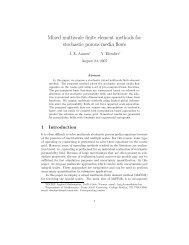
7Figure 4. Representation of one of the horizon surfaces of a geologicallayer. Main vertical faults are shown as green bands. Lateral coordinateaxes represent longitudinal and latitudinal coordinates. Verticalaxis represents depth below sea level, and the levels are indicated bythe contours on the horizon surface.A single injection well is used in the simulations to account for the injectedCO 2 corresponding to the location where injection is most likely to be performed.This penetrates the whole Johansen formation (vertically) at the chosenlocation. The positioning of an injection well is discussed in more detailbelow. The injection rates will be set to 3.5M tonnes CO 2 per year. This issomewhat more than the combined CO 2 emissions from Kårstø and Mongstad.The geological model for the Johansen formation and the sedimentary sequencesabove and below are based on geologist’s interpretations of horizons ofgeological layers, see Section 2. An example of an interpretation of one horizonis shown in Figure 4 together with the main vertical faults of the model. Withinthe layers, geological modelling has been performed. Petrophysical data, suchas porosity and permeability, has been modelled from seismics and by well correlations.At the time of making the data available, no geological facies modelwas available. A geological grid is constructed from the definition of horizonsof geological layers. Specifically, the main sequence of geological zones from topto bottom is given by:(1) Top Sognefjord(2) Sognefjord shale(3) Fensfjord formation(4) Krossfjord formation(5) Krossfjord-Brent group(6) Brent group(7) Dunlin group(8) Johansen formation (thickness varies between 80 m and 120 m).(9) Amundsen shale

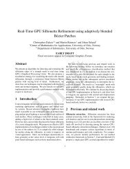
8 EIGESTAD, DAHLE, HELLEVANG, RIIS, JOHANSEN, AND ØIANqFigure 5. Permeability representation shown within sector of Johansenformation. Shale above and below Johansen are representedby 5 and 1 grid layers respectively.(10) Statfjord formationSome of these are divided into sub-zones so that the total model consists of16 geological zones. In particular, the Johansen formation contains three subzones.The lateral extent of the entire model is approximately 75 km × 100km.To limit the number of active grid cells in our study, CO 2 injection is simulatedonly in the sector model shown in Figure 5. This sector consists ofthe lower 3 geological zones (Amundsen, Johansen, Dunlin). Figure 5 showsthe permeability description within the sector model, where the Johansen formationhas been represented by 5 layers of grid cells. The lowermost layercorresponds to the Amundsen shale, and the 5 layers above Johansen correspondto the grid representation of the Dunlin shale. Notice the main faultthat divides the Johansen into two parts. The location of the injection well isin the area south-west of the the main fault and where CO 2 may move intothe areas to the east of the fault. Since the geological model indicates that thefaults are sealing when the fault throw is large we do not consider vertical flowin the faults towards shallower regions. Flow of CO 2 through the vertical faultshas been investigated in [6] by incorporating fault transmissibility multipliersin their model, and studying injection points further north, closer to Troll. Theoriginal dataset and corresponding grid, are made available on the web-site [11],and may be used to investigate faults as pathways for leakage in further studies.The actual position of an injection well for full scale CO 2 handling has notbeen decided yet. Currently seismic modeling is performed to get better data forgeophysical properties of Johansen, and these will be important for the choiceof injector position. Issues to be considered when choosing an injection point

are related to injectivity, to CO 2 not flowing into higher parts of the formation,and also to avoid CO 2 moving into areas near faults with uncertain sealingproperties. The location of the Troll field will also affect the choice of injectionpoint.Within both the Dunlin shale and the Amundsen shale, constant values areused for permeability; respectively 0.01 mD and 0.1 mD (1D = 9.86910 −13 m 2 ).The permeability of the Johansen formation varies between 64 and 1660 mD.The permeability data are based on well interpretation, and depth correlationsas described in Section 2. Figure 5 shows the vertical grid representation (withpermeability values) at a cross section within an extracted sector model, seenfrom west toward east.The grid is represented in corner point format [25]. This format is an extensionof the logical Cartesian grid format. Due to the vertical faulting ofgeological zones seen from Figure 5, the corners of grid cells are in general notconforming from one grid block to the neighboring grid block. The corner pointformat assumes that grid cell corners are distributed along vertical pillars. Allgrid cells have 8 corners, but these may not be distinct due to grid pinch-outs.Since the grids are allowed to contain vertical faults, all the eight corners areprovided for each grid block. This results in voluminous data. Section 3.3 containsa listing of the files where the geometry of the grids are provided. Gridsare provided for both the entire model and the sector model seen in Figure 5.The coarsest grid used in the simulations is a 100 × 100 × 11 corner point grid.The typical cell size for this grid is 500m × 500m laterally, and 16 to 24 mvertically.93.1. Discretization techniques. The simulations presented here are basedon the industry standard black oil simulator Eclipse 100 [12]. This simulatoris based on a control-volume formulation of the governing equations. In thisformulation each grid block i will be a control volume V i such that mass balanceis satisfied for each fluid phase α:(1)∫( ∂(φρ α)V i∂t∫+ ∇ · (ρ α v α ))dV = q α dV,V iwhere the following quantities are introduced: φ porosity; ρ α phase density; q αsource or sink terms for fluid phase α. The Darcy velocity v α for phase α isgiven by(2) v α = − Kk r αµ α(∇p + ρg∇z).Here K is the permeability/conductivity of the porous medium, k rα is therelative permeability for phase α, µ α is the viscosity of phase α, p is the pressure,g is the gravitational constant, and z denotes the height above some depthreference point. Capillary pressure is neglected for simplicity.We will consider three types of boundary conditions. These are introducedin Section 4.2 together with their practical implemetation.

10 EIGESTAD, DAHLE, HELLEVANG, RIIS, JOHANSEN, AND ØIAN3.1.1. Transmisibility calculations. Fluxes are discretized for all cell faces of agrid block. A common discretization technique, e.g. used in [12], is the twopointflux approximation (TPFA) method. In this method single phase fluxesacross grid block faces are be approximated by(3) f i = t i (u i− − u i+ ),where u i− and u i+ refer to the fluid potentials at the grid block nodes oneither side of the grid block face. The coefficient t i denotes the transmissibilityassociated with the grid block face, and is essentially calculated from localgeometry and permeability, cfr. [1]. Multi phase flow is handled by upstreamweighting of relative permeability. When the grid blocks are faulted with respectto each other, the transmissibility coefficients are modified, see [2], [3], [17], andlarger cell stencils for the discretized mass balance equations may occur. If thereis communication between layers that have been faulted with respect to eachothers through faults, so-called non-neighbour connections may be set up. Thismeans that the indexing of the fluid potentials in Eq. (3) may be generalized toaccount for grid cells that are not ’logical’ neighbors, so that flows across gridblock faces are governed by non-neighbouring cells.Multi point flux approximation methods (MPFA), are more general transmissibilitycalculation techniques when more grid block/control volumes are usedto approximate fluxes, see [1], [2], and [3].The concept of transmissibility multipliers allows for modifications of thediscrete fluxes in Eq. (3), see for example [17], and is often used for historymatching in practical reservoir simulation. The transmissibility t i is multipliedby a factor to either increase or decrease the flux across the cell phase. Layersthat are ’neighbours’ across a fault, may be assigned a small transmissibilityif flow is reduced across the fault. The faults in our simulation grids arepredominantly sealing due to the high clay content in Dunlin shale, so thattransmissibility reduction factors are used in Eq. (3). The dataset containsfiles with transmissibility multipliers produced from the fault handling in [12].Various methods exist for calculations of transmissibility multipliers based onlocal geometry in the vicinity of the faults and the local geological properties.More detailed knowledge of the geology, such as clay content, fault smearing,fault throw and orientation of fault zones may also be included in calculationsof multipliers [17]. In Figure 6 we have shown calculated fault transmissibilitymultipliers for the main faults, based on clay content and fault displacementfrom the entire geological model.An example of fault transmissibility multipliers for the sector model is providedin Figure 7, which shows multipliers for the part of the main fault betweenthe layers included here.Fault activation due to pressure build-up constitutes potential risks for leakageout of the formation, [4]. In the case of the Johansen formation, CO 2may then flow to layers of sandstone above the formation, and further up tothe Troll field or surrounding media. Leakage of CO 2 to the formations abovethe Johansen formation has been investigated in [6] by studying various faulttransmissibility options for a full model.

11Figure 6. Fault transmissibility multipliers calculated for the majorfaults in the full geological model, as seen in Figure 4, based onclay content of Dunlin shale in combination with Johansen sandstoneproperties and fault throw.Figure 7. Transmissibility multipliers of the faults used in the sectormodel. Horizon of one of layers shown together with discrete representationof vertical faults.3.2. Fluid data. The dataset presented here provides geometry, geology andpetrophysical properties for a realistic storage site. We consider two-phaseimmiscible flow with CO 2 being the nonwetting phase, and the resident brine

12 EIGESTAD, DAHLE, HELLEVANG, RIIS, JOHANSEN, AND ØIANFigure 8. Relative permeability curves for CO 2 and water, withresidual brine saturation, S rb = 0.1, and residual CO 2 saturation,S rc = 0.2.being wetting. The phases are isothermal, compressible, and have densities andviscosities that vary with pressure. Isothermal PVT data at 94 degrees Celsiusare generated from the web-based database NIST [16] for pressure values inthe pressure regime that exists during the simulation time. As an example, at250 bar pressure supercritical CO 2 has a density of approximately 617 kg/m 3 ,and viscosity 0.049 cP. This should be compared to water density of 973 kg/m 3and water viscosity of 0.307 cP for 250 bar. Tables with varying PVT dataare further presented in the online data-set [11], and a description of the files isprovided in Section 3.3. Relative permeability data consists of a set of water andCO 2 curves, where the residual water saturation is S rb = 0.1 and residual CO 2saturation is S rc = 0.2. The relative permeability curves for water and CO 2used in this dataset are plotted in Figure 8. In this study we do not accountfor hysteresis in residual CO 2 saturation values which generally depends onthe sweeping history, see for instance [13]. However, the effect of varying theend-points of the relative permeability curves is investigated in Section 4.4.Capillary pressure has been neglected in this study, but it should be emphasizedthat core data treatment to determine both relative permeability andcapillary pressure is an important issue, and of particular interest for long termbehavior, and fluid propagation after the injection phase.3.3. Data file descriptions. Datafiles are made available on the web-page[11]. A brief description of datafiles is provided below. The web page will containa more detailed description of data included and specific files. Additionalinformation is also included in file headers.Geometry files:Grids are made available in corner point format, see [25]. The entire model isdiscretized by a 155 × 160 × 16 grid. This grid describes all zones and theentire lateral domain. The Johansen formation is given by 3 layers.The sector models correspond to the south western parts of the geological domain.The sector models are discretized by a 100 × 100 lateral grid and by

(1) 5 layers, (2) 10 layers, (3) 15 layers representation of Johansen formation.The shale (Dunlin) above Johansen is represented by 5 grid layers in all sectormodels.Petrophysical data files:Petrophysical data is given for the entire model, and for the sector models withdifferent vertical grid representation corresponding to geometry files above.Fault data files:Logical fault definitions are given corresponding to files above. Non-neighbourconnections and fault transmissibility multipliers are provided for the differentgrids.Fluid data files:Fluid data is given for an immiscible water-CO 2 system at isothermal conditions.PVT data is given for 94 degrees Celsius.Well data files:Well positioning is given in global coordinates. The rates are constant duringthe injection period, and the well has vertical perforation through the Johansenformation.134. Simulation of CO 2 injection in the Johansen aquiferThe aim of this Section is to study some modeling factors that we believeare important for the CO 2 saturation distribution in the formation, and consequentlyfor the storage capacity estimation. For a complete study of storage ofCO 2 and risk modeling, a much more detailed study must be performed.The sector model includes shale both above and below the Johansen formationitself. In particular, the Johansen formation is limited upwards by theDunlin shale/group, see Section 2 for more details.All examples are simulated with the Eclipse 100 simulator [12]. Simulationsare performed for various grid representations of the sector domain. Boundaryconditions and permeabilities will be specified for the various examples.Fluid data is described in Section 3, and is the same for all examples. Faultsand transmissibility calculations are handled internally in the simulator for thevarious geometry and permeability files. The initial water pressure for the simulationsis assumed to be determined by hydrostatic equilibrium, indicatingpressures around 250-310 bar within the simulated sector model. Fluid flow issimulated on a lateral sector of the geological model in the south-westernmostpart of the Johansen formation. This sector is described in detail in Section 3.Initially we give an example of simulation of CO 2 injection in the Johansenformation, together with a simplified CO 2 inventory study. Then the effects oflateral boundary conditions, grid resolution, and relative permeability descriptionare studied. Finally some simulations with varying permeability modelsare presented.

16 EIGESTAD, DAHLE, HELLEVANG, RIIS, JOHANSEN, AND ØIANFigure 10. CO 2 saturation development for simulation set-up inSection 4.1 in upper grid layer of Johansen. Uppermost plot; saturationprofile after 110 years (injection stop). Middle plot; 210 years.Lowermost plot; 510 years. Notice that CO 2 reaches the main verticalfault during the simulation period, which may constitute leakagescenarios higher up in the formations through the fault.permeability of the grid cell, n is the outward normal vector of thebounday face, and u is the fluid potential.BC2: Grid cells at parts of the lateral boundary are assigned pressuredriven production wells, while the boundary edges of boundary cellsemploy a no-flow condition. The constraints on the artificial wells are

17Figure 11. Amount of CO 2 within box region surrounding injectionwell vs. time. Amount increases linearly with the injection rate untilCO 2 reaches boundary of the box region. Afterwards a decrease isobserved. Asymptotic trend indicates effect of trapping of CO 2 withinthe box, and is a combination of residual trapping and stratigraphictraps.set such that almost the same injected volumes are being producedinitially. This relies on modification of the well term q of Equation (1)for cells containing wells. Specifically, here we employ two productionwells (pressure driven, constant pressure of 270 bar) near the main fault,in the western part of the Johansen area. The reason for choosing thesepositions is to show the possible communication with layers higher inthe formation through the main vertical fault by triggering movementof CO 2 towards the areas near the main fault.BC3: Boundary conditions specified through reservoir contact with externalaquifers. This boundary treatment option is commonly used in practicalreservoir simulation. The aquifer contact can be represented eithernumerically or analytically. In the analytical case, the aquifer is representedthrough source terms in a specified set of boundary grid cells.Various models exist for computing the source terms. In our case, wehave used the Fetkovich aquifer model which assumes a pseudosteadystateflow regime between the aquifer and the reservoir. The aquiferinflow rate is specified by a Darcy law type expression, while the pressureresponse in the aquifer is given by a material balance expression.We refer to [12] for more details on external aquifer representation.In Figure 12 the bottom hole pressure (BHP) for the injection well has beenplotted versus time for the simulations with the boundary conditions above.The medium is described by homogeneous permeability (500 mD), and a 10layer grid representation is employed throughout the Johansen formation. Relativepermeability curves are shown in Figure 8, and the fluid data is the sameas in Section 4.1. As can be seen from the plot, the BHP initially experiencesa sharp transient response lasting for about 5 years. This transient consistsof a rapid pressure increase of approximately 10-12 bar followed by a pressuredecrease. A slow long term increase of the BHP in Figure 12 is due to

18 EIGESTAD, DAHLE, HELLEVANG, RIIS, JOHANSEN, AND ØIANFigure 12. Bottom hole pressure (BHP) versus time for differentboundary conditions: Red curve corresponds to no-flow boundarieswith increased pore volumes at boundary cells (BC1); Blue curve toflux/pressure control in boundary cells (BC2); Green curve to aquifersupport (BC3).net accumulation of fluid inside the formation. Although these conditions givecomparable results we note that the aquifer support condition, BC3, gives thelowest BHP increase. This, however, depends on how the aquifer options areapplied [12]. The formation pressure build-up may be a very important sinceit can lead to fracturing and fault activation, see for example [6].The CO 2 saturation distributions after 510 years simulation for each of theseboundary conditions are shown in Figure 13. As can be seen from the figure,there is little difference between the case with pore volume multipliers andthe external aquifer support, BC1 and BC3 respectively. In these cases theCO 2 saturation distributions are determined mainly by buoyancy effects, localtopology of the layers, and the inherent effect from juxtaposition of layers andthe impermeable cell faces of these due to shale in the faults. As expected theCO 2 saturation for the flux/pressure condition (BC2) is quite different fromthe results obtained using the other types of boundary conditions. This resultdoes not only depend strongly on the conditions chosen for each of the artificialwells, but also on their location. In this case, since the location of the artificialproducers is at the western part of the main fault, more CO 2 moves into thewestern part of the formation.4.3. Grid resolution and distribution of CO 2 plume. Due to computationaldemands on the fluid flow simulator, the issue of grid coarsening arisesnaturally and will limit the number of grid cells used in a simulation model.Whereas the geological grid may contain much more detailed information about

Figure 13. CO 2 saturation distributions after 510 years (110years of injection; thereafter 400 years post injection period).Uppermost figure corresponds to no-flow boundaries with increasedpore volumes at boundary cells (BC1). Middle figurecorresponds to flux/pressure control in boundary cells (BC2).Lowermost figure corresponds to aquifer support (BC3). Homogeneouspermeability description (500 mD), 10 layer grid representationof Johansen. Grid lines are not included for visualizationpurposes.19

20 EIGESTAD, DAHLE, HELLEVANG, RIIS, JOHANSEN, AND ØIANgeometry and geology of the formation, geometry and permeabilities must eventuallybe up-scaled to a representative simulation grid. An important issue toconsider from a modelling and simulation perspective is the effect that coarseninghas on the CO 2 saturation distribution when accounting for relative permeability,capillary pressure and PVT data. The shape of CO 2 plumes has beenstudied, e.g. in [18], [19], [20], and suggests that a certain level of grid resolutionmust be employed to incorporate the effects of nonlinearities. In particular, wemust expect to provide sufficient grid resolution in the vertical direction.To simplify the study of grid resolution effects on the CO 2 saturation distribution,we use homogeneous permeability within the Johansen formation andthe neighbouring layers. The permeability is set to 500 mD in Johansen, andlow permeability values are used for the Dunlin shales/group as described inSection 3.The shales above and below the Johansen formation are represented respectivelyby 5 and 1 layer(s) of grid cells. Within the Johansen formation weconsider three different vertical grid resolutions in the 5 layer model, and weinvestigate different local grid resolutions in the areas which will be flooded byCO 2 . The areas with local grid refinement (LGR) are the same as in Figure 9.The first grid has no refinement, the second has 2 × 2 local refinement laterally,and 4 cells vertically. The third grid has local refinement 3 × 3 laterally, and 8cells vertically.In Figure 14 the simulation cases are presented. The CO 2 saturation distributionin the top layer is plotted after 110 years of injection followed by a400 year post-injection period. As can be seen from the plots, the distributionof CO 2 differs significantly. The lateral spreading of CO 2 in the uppermostlayer of the Johansen formation covers a much larger area when using the finergrids. The major difference is between coarse grid and the refined grids. Thedifference between the 2 × 2 × 4 LGR and 3 × 3 × 8 LGR is much smaller, andindicates that the 2 × 2 × 4 LGR representation in the upper layer is reasonablyaccurate for simulation of CO 2 injection in this particular case. Note, however,that we have not performed a detailed convergence study of the grid resolutions.Although this example mainly accounts for flow within the Johansenformation, grid resolution issues are important to be aware of when simulatingCO 2 movement in a full model. Needless to say, if a high level of grid refinementis needed in the simulation grids, the computational demand may be severe.It is observed in the simulations that some CO 2 migrates up into the firstlayer immediately above Johansen. After 510 years the maximum saturation inthis grid layer of shale is approximately 5 percent. In the grid layers above weobserve no CO 2 . The reason why CO 2 moves into the shale in the numericalsimulations is dependent on the relative permeability representation. Specifically,since upstream weighting of relative permeability is used by the simulator,some of the CO 2 movement into the shale is a purely numerical effect. Thisdiscretization technique then leads to an over-estimate of CO 2 volumes in thelower parts of the shale. Due to the very low permeability values at saturationvalues near critical CO 2 saturations, the movement of CO 2 to the shale gridlayers higher in the formation will be almost zero. In our relative permeabilitymodel, as indicated by Figure 8, the relative permeability values at 5 percent

Figure 14. Simulation of CO 2 migration with various grid resolutionin the uppermost layer of the Johansen formation. CO 2 profileafter a total simulation period of 510 years. Uppermost plot; 5 gridlayer representation of Johansen with no refinement. Middle; 5 layerscombined with local grid refinement factor of 2 laterally and 4 verticallyin upper grid layer. Lowermost plot; 5 layers combined withlocal grid refinement factor of 3 laterally and 8 vertically in upper gridlayer. Grid lines not plotted for visualization purposes.21

22 EIGESTAD, DAHLE, HELLEVANG, RIIS, JOHANSEN, AND ØIANare actually zero, and no movement further up in shale is seen. Since we haverepresented the shale by 5 grid layers here, this impairs overestimated volumesof CO 2 higher in the shale zones. Grid representation of shale will also affectthe CO 2 movement/migration in a full field model where transport of CO 2 isallowed due to fault transmissibility modifications, and care must be taken notto make conclusions about CO 2 migration and leakage that are biased by thenumerical simulation techniques.4.4. Impact of relative permeability. To illustrate the effect of residual saturation,the saturation distributions at the time when injection is stopped (110years) is compared with the distribution 100 years later. The simulation gridis the 10 grid layer representation of Johansen with homogeneous permeability.Relative permeability curves from Figure 8, and BC1 have been employed.Two notable effects are seen from the plots in Figure 15. After end of injection,CO 2 will continue to move upwards due to buoyancy, and displacewater. In the plotted regions, CO 2 has flooded areas close to the injectionpoint. When CO 2 continues to move upwards from flooded areas, CO 2 willeventually be trapped due to the residual CO 2 saturation value used in thedefinition of relative permeability curves. This leaves a trail of residual andimmobile CO 2 phase, as seen in Figure 15. In our example calculations theresidual CO 2 saturations are set to 20 percent. However, experimental valuesclose to 40 percent have been reported in the literature [4]. Storage capacityestimation is of course very sensitive to the value of residual CO 2 saturation.Rock property models may be a major uncertainty for North Sea geologicalformations. The effect of varying relative permeability data is illustrated bythe following example. Consider the relative permeability curves (1), (2) and(3), shown in Figure 16, with curve explanation in the figure text. The fluiddata is the same as the previous examples, homogeneous permeability of 500mD and 10 grid layers are used for Johansen. Saturation profiles are plottedin Figure 17 for each case. As seen from the figures, the fronts spread quitedifferently depending on the permeability description. The most spreading ofCO 2 is seen when using the relative permeability Curve (2). This relative permeabilitycurve is obtained by scaling Curve (1) corresponding to the originalrelative permability curve for CO 2 given in Figure 8 by a factor 2. Larger areaswill also be swept by the primary drainage Curve (3) compared to the originalrealtive permeability Curve (1), since no residual CO 2 is left in place in thiscase. In this case we also observe that more CO 2 moves into the parts westof the main fault. The relative permeability description will be important forleakage scenarios since the end-points and form of these curves alters the frontspeed and sweep areas of the CO 2 plume. This may lead to faster arrival topotential pathways upwards in the formation, and possibly also faster migrationin faults.The effects of relative permeability hysteresis for CO 2 modelling are studiedin [13]. Mainly hysteresis will alter the shape and speed of the propagatingfront. From Figure 16 we see that the relative permeability of CO 2 is largerwhen S rc = 0 (Curve (3)) than when S rc ≠ 0 (Curve (1)). Consequently, thefront of the CO 2 -plume will flow faster when the residual CO 2 is zero. This is

23Figure 15. CO 2 saturation distribution in a region near the injectionpoint. Upper Figure: CO 2 saturations after 110 years of injection.Lower Figure: CO 2 saturations 100 years after injection was stopped.Residual CO 2 saturation of 20 percent, and curves from Figure 8 applied.Approximate thickness of grids cells is 8-10 meters.also observed in the simulations. The effect of trapping in a hysteresis modelas compared to a model with fixed residual saturation, S rc ≠ 0, see Figure 8,would primarily be that less CO 2 may be trapped when the hysteresis curvesare used. For areas that have been flooded by CO 2 , but where maximum CO 2saturation has not been reached, the residual CO 2 saturation will be less thanS rc if drainage is reversed to imbibition for these grid blocks.4.5. Impact of permeability description. The chosen injection point inthis study is in the south-westernmost location of the Johansen formation. Theheterogeneous permeability model described in Section 2 was employed in thesimulation example in 4.1. Possible injection positions further north toward

24 EIGESTAD, DAHLE, HELLEVANG, RIIS, JOHANSEN, AND ØIANFigure 16. Different relative permeability curves for CO 2 : Curve(1) is identical to the curve given in Figure 8 with residual brine saturationS rb = 0.1, and residual CO 2 saturation, S rc = 0.2; Curve (2)is obtained by shifting the end-point relative permeability at residualbrine saturation by a factor of 2 (this scales Curve (1) by a factor2); Curve (3) represents primary drainage and is obtained by shiftingresidual CO 2 saturation to S rc = 0;the Troll area would be in regions with higher permeability values in the geological/geophysicalmodel. This motivates testing different permeability descriptionswith larger values in this example. We employ the 5 layer simulationgrid for the Johansen formation, described in Section 3. Local refinement isused in the same areas as in Example 4.1, and relative permeability curve (1)is taken from Figure 16. The first permeability model is the heterogeneousmodel from Example 4.1, the second uses homogeneous permeability of 500mDin the entire area of Johansen, and the third used homogeneous permeability of1000mD. The simulated CO 2 profiles are plotted in Figure 18. As can be seen,the front moves much further with the largest values for the permeability, andmuch larger areas are swept by CO 2 . As a consequence, the effects of residualCO 2 trapping are much more profound for larger values of permeability, andseveral local domes are observed with CO 2 trapped in stratigraphic traps. Froma storage point of view, the trapping effects have a positive effect. However, dueto sweeping larger areas, there is an increased risk of CO 2 moving into morefaulted regions where leakage into formations above the Johansen formationcould occur.5. ConclusionsThe Johansen formation is a deep saline aquifer located offshore the westcoast of Norway. The aquifer is a candidate site for large-scale handling of CO 2emissions from future gas power plants. This paper describes a dataset for thegeological model. The dataset can be dowloaded together with fluid properties.The geological model has been described in detail, and some simulation resultshave been shown for injection of CO 2 . These simulations have been performedusing the industry standard simulator Eclipse 100, and can be used as a basis

25Figure 17. CO 2 saturation profiles simulated with the three differentrelative permeability curves shown in Figure 16. Simulated profilesplotted in uppermost grid layer of Johansen after 110 years of injectionfollowed by 400 years of post injection. The top figure corresponds toCurve (1) in Figure 16; The middel figure to Curve (2); The bottomfigure to Curve (3);for comparisons. The geological model has been used to perform various simulationsof CO 2 flow and transport based on realistic injection scenarios. Weshow that the choice of lateral boundary conditions may significantly changethe simulation results. Furthermore, we show that vertical grid refinement is

26 EIGESTAD, DAHLE, HELLEVANG, RIIS, JOHANSEN, AND ØIANFigure 18. CO 2 saturation distributions after 510 years of simulationfor three different permeability representations of the Johansenformation. Saturation profiles plotted in the top grid layer of Johansen.Top; heterogeneous permeability model. Middle; homogeneous permeabilitymodel with 500mD. Bottom; homogeneous permeability modelwith 1000md.needed to properly resolve the CO 2 plume. The numerical example calculationsillustrate important trapping mechanisms. In particular residual gas saturationand stratigraphic traps are considered. The spreading of CO 2 is highly dependenton the relative permeability models that are used. Local domes in

combinations with cap-rock and sealed faults may provide significant practicalstorage volumes, provided that the integrity of the cap-rocks and faults canbe verified. The impact of permeability description has been discussed and isshown to have significant effect on the simulated saturation distributions.6. AcknowledgmentsThis work was supported by the Norwegian Research Council, Statoil Hydro,and Norske Shell under grant no. 178013/I30.References[1] Aavatsmark, I, E. Reiso, R. Teigland (2001), Control-Volume Discretization Methods forQuadrilateral Grids with Faults and Local Refinement, Computational Geosciences 5, pp1-23.[2] Aavatsmark, I., E. Reiso, H. Reme, R. Teigland (2001), MPFA for Faults and Local GridRefinement in 3D Quadrilateral Grids With Application to Field Simulations, SPE 66356,Proceedings of SPE Reservoir Simulation Symposium, Houston, Texas.[3] Aavatsmark, I., G.T. Eigestad, B.-O. Heimsund, B. Mallison, J.M. Nordbotten, E. Øian(2007), A New Finite Volume Approach to Efficient Discretization on Challenging Grids,SPE 106435, Proceedings of SPE Reservoir Simulation Symposium, Houston, Texas.[4] Bachu S. (2008), CO 2 storage in geological media: Role, means, status and barriers todeployment, Progress in Energy and Combustion Science, 34, pp 254-273[5] Bachu S., D. Bonijoly, J. Bradshaw, R. Burruss, S. Holloway, N.P. Christensen, and O.M.Mathiassen (2007), CO 2 storage capacity estimation: Methodology and gaps, Int. Journalon Greenhouse Gas Control, 1, pp 430-443[6] Bergmo, P.E, E. Lindeberg, F. Riis, W.T. Johansen (2008), Exploring geological storagesites for CO 2 for Norwegian gas power plants: Johansen formation, Proceedings ofGHGT-9, 16.-20. November 2008.[7] Bradshaw J., S. Bachu, D. Bonijoly, R. Burruss, S. Holloway, N.P. Christensen, andO.M. Mathiassen (2007), CO 2 storage capacity estimation: Issues and development ofstandards, Int. Journal on Greenhouse Gas Control, 1, pp 62-68[8] Class, H., H. Dahle, F. Riis, A. Ebigbo, and G. Eigestad (2008), Estimationof the CO 2 Storage Capacity of a Geological, Numerical Investigationsof CO 2 Sequestration in Geological Formations: Problem Oriented Benchmarks,http://www.iws.uni-stuttgart.de/CO 2-workshop/[9] Gassnova (2007), Beslutningsgrunnlag knyttet til transport og deponering av CO 2 fraKårstø og Mongstad, Report no 06/177, (In Norwegian)[10] Ebigbo A., J.M. Nordbotten, and H. Class (2008), CO 2 Plume Evolutionand Leakage through an Abandoned Well, Numerical Investigations ofCO 2 Sequestration in Geological Formations: Problem Oriented Benchmarks,http://www.iws.uni-stuttgart.de/CO 2-workshop/[11] Eigestad, G.T, H. Dahle, B. Hellevang, W.T. Johansen, K.-A. Lie, F. Riis and E.Øian (2008), Geological and fluid data for modelling CO2-injection in the Johansen formation,http://org.uib.no/cipr/Project/MatMoRA/Johansen/index.htm (to be madeavailable)[12] Sclumberger (2006), Eclipse 100/300 Reference Manual and Technical Manual[13] Juanes, R., E.J. Spiteri, F.M. Orr Jr., and M. J. Blunt (2006), Impact of relative permeabilityhysteresis on geological CO 2 storage, Wat. Res. Research, 42[14] Lindeberg, E., P. Zweigel, P. Bergmo, A. Ghaderi, and A. Lothe (2001), Prediction ofCO 2 distribution pattern improved by geology and reservoir simulations, Proceedings ofthe Fifth Int. Conf. on Greenhouse Gas Reduction Technologies[15] Lindeberg, E., and P. Bergmo (2003), The long-term fate of CO 2 injected into an aquiferPrediction, Proceedings of the Sixth Int. Conf. on Greenhouse Gas Reduction Technologies27

28 EIGESTAD, DAHLE, HELLEVANG, RIIS, JOHANSEN, AND ØIAN[16] NIST Chemistry web-book, http://webbook.nist.gov/chemistry[17] Manzocchi, T., J.J. Walsh, P. Nell and G. Yielding (1999), Fault Transmissibility Multipliersfor Flow Simulation Models, Petroleum Geoscience, 5, pp 53-63[18] Nordbotten, J. M. and M. A. Celia (2006), An improved analytical solution for interfaceupconing around a well, Water Resources Research, 42[19] Nordbotten, J. M. and M. A. Celia (2006), Similarity Solutions for Fluid Injection intoConfined Aquifers, Journal of Fluid Mechanics, 561, pp 307-327[20] Nordbotten, J. M., M. A. Celia, S. Bachu and H. K. Dahle (2005), Semi-AnalyticalSolution for CO 2 Leakage through an Abandoned Well, Environmental Science and Technology,39(2), pp 602-611[21] Nordbotten, J. M., M. A. Celia and S. Bachu (2005), Injection and Storage of CO 2 inDeep Saline Aquifers: Analytical Solution for CO 2 Plume Evolution During Injection,Transport in Porous Media, 58(3), pp 339-360[22] Nordbotten, J. M., M.A. Celia and S. Bachu (2004), Analytical Solutions for LeakageRates Through Abandoned Wells, Water Resources Research, 40[23] Schlumberger (2007), Petrel Reference Manual[24] Torp, T.A., JJ. Gale (2004), Demonstrating storage of the CO 2 in geological reservoirs:The Sleipner and SACS projects, Energy 29, pp 1361-1369[25] Ponting, D.K. (1992), Corner Point Geometry in Reservoir Simulation, Proceedings ofthe 1st European Conference on the Mathematics of Oil Recovery, Cambridge, ClarendonPress, Oxford, pp 45-65.[26] Pruess, K., T. Xu, J. Apps, J. Garcia (2003), Numerical Modeling of Aquifer Disposal ofCO 2, SPE 8 (1), pp. 49-60.(Geir Terje Eigestad) Dep. of Mathematics, University of Bergen/Perecon AS, Bergen, NorwayE-mail address: geirte@math.uib.no(Helge K. Dahle) Dep. of Mathematics,University of Bergen, NorwayE-mail address: helge.dahle@math.uib.no(Bjarte Hellevang) Reslab Integration,Bergen, NorwayE-mail address: bjarte.hellevang@ri.reslab.no(Fridtjof Riis) Norwegian Petroleum Directorate,Stavanger, NorwayE-mail address: Fridjof.Riis@iris.no(Wenche Tjelta Johansen) Norwegian Petroleum Directorate,Stavanger, NorwayE-mail address: Wenche.Johansen@npd.no(Erlend Øian) Perecon AS,Bergen, NorwayE-mail address: erlend.oian@perecon.no