Analysis of Fluorescence Decay by the Nonlinear Least Squares ...

W using excitation function A. The following values were
used for the parameters in Eq. (15): Al = 10.0, rI = 0.1 ns,
A2 = 1.0, and r2 = 2.0 ns. Ten sets of excitation and
emission data were simulated for each W. Deconvolution
analysis by method I produced consistently better results
(i.e., A1/A2, and rI were closer to the values used in
simulation) compared with method II for all W; however,
for W < 1 x 104, the analysis by both the methods gave
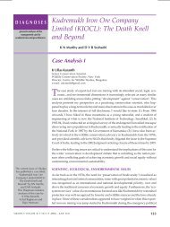
chi-square values which are nearly equal. Fig. 2 shows the
variation of the chi-square values obtained in the analysis
by method I and II as a function of W. The data analysis by
either method gave a chi-square value which increased
with increasing W, the increase being steeper in the case of
method II. This indicates that the numerical integration
proposed here is better than the trapezoidal approximation
for handling precision data.
Methods I and II were then compared with the analysis
of data simulated for various values of the short lifetime
component. The simulation parameters were as follows:
W = 105, A2 = 1.0, r2 = 2.0 ns, and AI = 10.0. ,r was varied
from 0.02 to 1.0 ns. For each value of rI ten sets of
excitation and emission data were simulated. These simulation
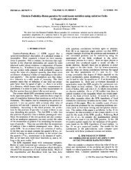
data were analysed and Fig. 3 A shows the variation
of the chi-square values obtained by both the methods. Fig.
3 B shows the ratio (rI/rI) obtained by both the methods,
IT being the average of ten optimised values ofTI obtained
in the analysis. It is found that method I is able to extract
the short lifetime component more correctly and with
better values for statistical test parameters. However, for
T1 > 0.5 ns both the methods are equally efficient.
The randomness of the distribution of weighted residuals
is usually checked by the calculation of reduced chisquare
and other test parameters. It is instructive to
examine also visually the distribution of the weighted
w
I I()
3-0 -
201-
1-0 _
0-0
103 104
s _A _R
10w
W
10°
FIGURE 2. Variation of the values of chi-square obtained by method I
(o) by method II (x) for various values of W. See text for details.
966
4 I]
I I
_S!~~I
0
1 5 _ B
*-0
1-0
wI
X 1-4
I
C) 10
x
x
-90 6 K K
x x
x
x
0
0.0
II
0-5
T. (ns)
1-0
A
FIGURE 3. Plot of optimised
values (average of ten) of the
short lifetimes (rl) (plotted as
ll/r1, top) and chi-square (bottom)
obtained in the analysis of
data by method I (o) and by
method 11 (x) versus Tx. bt = 50
ps for all simulated data. See text
for details.
residuals. Fig. 4 shows a typical display of the weighted
residuals obtained by methods I and II in the analysis of
simulation data using Eq. (11) for excitation function
(cr = 0.2 ns, m = 1.2 ns, and W= 1 x 105), and Eq. (15)
for I(t) (AI = lO.O,T1 = 0.1 ns,A2 = 1,andT2 = 2ns). The
simulated excitation data, emission data, and fitted emission
data (method I) are shown in Fig. 4. In this case the
emission data was not normalized and the peak count
was -1.2 x I05. The distribution of the weighted residuals
in the region dominated by the short lifetime component is
more acceptable in Fig. 4 B than in Fig. 4 C. Deconvolution
by method I produced the following results: AI = 10.0,
Tr = 0.101 ns, A2 = 1.01, T2 = 2.00 ns, (reduced) chisquare
= 1.17, Durbin-Watson parameter (DWP) = 1.90,
standard normal variate of runs test (Z) = -0.05, and
percentage of weighted residuals between -2 and + 2
(PER) = 95.09. Deconvolution by method II produced the
following results: AI = 9.44, T1 = 0.106 ns, A2 = 1.01, T2 =
2.00 ns, chi-square = 1.41, DWP = 1.59, Z = 1.58, and
PER = 92.77.
In the simulations described earlier the time interval was
chosen to be 50 ps. The conclusion that the performance of
method I is better than method II when the short lifetime
in the decay equation is comparable to bt is independent of
the value of bt used in simulations. The computation time
required for method I or method II depends upon the
number of iterations required for convergence, which need
not be equal. On the average it is observed that method I
requires -10% more computer CPU time (Cyber 170/
730) than that required for method II. However, there
were several cases in which method I required less time
than method II because of convergence at a lower interation
number.
The method proposed here has also been used in the
analysis of experimental fluorescence data of standard
samples obtained by time-correlated single photon
counting technique. In comparison with the simulation
data the quality of the experimental data was poor because
of system errors, especially the wavelength response of the
photomultiplier which needed to be corrected in the analysis
by introducing a shift parameter. In spite of this, it is
generally observed that method I generates results with
BIOPHYSICAL JOURNAL VOLUME 54 1988