Analysis of Fluorescence Decay by the Nonlinear Least Squares ...

BRIEF COMMUNICATION
ANALYSIS OF FLUORESCENCE DECAY BY THE
NONLINEAR LEAST SQUARES METHOD
N. PERIASAMY
Chemical Physics Group, Tata Institute ofFundamental Research, Homi Bhabha Road, Colaba,
Bombay: 400 005, India
ABSTRACT Fluorescence decay deconvolution analysis to fit a multiexponential function by the nonlinear least squares
method requires numerical calculation of a convolution integral. A linear approximation of the successive data of the
instrument response function is proposed for the computation of the convolution integral. Deconvolution analysis of
simulated fluorescence data were carried out to show that the linear approximation method is generally better when one
of the lifetimes is comparable to the time interval between data.
INTRODUCTION
Time-resolved fluorescence decay measurements provide
important information about the structure and dynamics
of the system under investigation. In a general application
the experimental fluorescence decay data is fitted to a
decay function, I(t), which is derived for an assumed
model. Nonlinear least squares method (1, 2) is generally
used in fitting the data to the function I(t) and one obtains
optimum values for the adjustable parameters in I(t). This
method requires numerical evaluation of the convolution
integral (Eq. [1]) and the partial derivatives of F(t) with
respect to the adjustable parameters. R(t) in Eq. (1) is the
instrument response function or excitation function.
F(t) = fr R(s) I(t - s) ds. (1)
When I(t) is a multiexponential function, Xi Ai exp (-t/
ri), Ai, and ri are the adjustable parameters. Grinvald and
Steinberg (3) proposed an algorithm based on the trapezoidal
approximation for the numerical integration. This
method is widely used, though other approximations
(Simpson's rule and law of the mean) are also found to be
equally good (4). In these approximations it is implicitly
assumed that the excitation function is a series of delta
functions separated in time. However, the pulsed light
sources employed in experiments are expected to have a
continuous variation of intensity with time and hence the
excitation function used in deconvolution ought to be
continuous. Here, we construct a continuous excitation
function using the discrete excitation data by assuming a
linear variation between the discrete data. Numerical
calculation of F(t) can then be carried out using integrated
expressions. The performance of this new method to calculate
F(t) is compared with that of Grinvald-Steinberg
BIOPHYS. J.© Biophysical Society * 0006-3495/88/54/961/07 $2.00
Volume 54 November 1988 961-967
method in the analysis of fluorescence data simulated
under various conditions.
MATHEMATICAL EQUATIONS
Consider that RI, . . . Ri, . . . Rn are the n numerical data of
the instrument response function and bt is the time interval
between R, and Ri-1. In the linear approximation R(t) is
considered as (n - 1) step functions (RI[t], R2[t],...
Rj[t] ... Rn_I[t]) represented by Eq. (2).
Rj(t) = mjt + cj, for i < t s (i + l)bt
= 0, otherwise (2)
m. and c; are the slope and intercept of the line joining R
and Ri-1. The convolution integral (Eq. [1]) can then be
written as,
i-l
Fi = EZf6 R1(s) I[(i - l)t - s] ds
j I (i- OWa
for i # 1. When I(t) is a sum of p exponentials,
I(t) = t Ak exp (-t/1Tk).
k-l
Eq. (3) is integrated to give the following recursion relation:
I= F1 exp (-bt/Tk) + AkTk {Ri - Ri-I
exp (-bt/Tk) - mi lTk [1 - exp (-bt/rk)]I (5)
Fi
p
= ik.
k-l
The partial derivatives of F(t) are given by Eqs. (7) and
(8) summed over all k.
(aFP/oAk) = (FI/A) (7)
(3)
(4)
(6)
961

(4F9/Ork) = exp (-&t/rk) [(OF,I/8Tk) + F 1(St/r2)]
+ A [Ri - Ri.l exp (-6t/Tk){1 + (t/rTk)I
- 2 miTk{l - exp (-bt/Tk)I
+ m,_, at exp (-bt/rk)]-
For i = 1, F Ak bt RI, (dFl/OAk) bt R, and (oFV/
9Tk) = 0. When R, = 0, which condition is usually met in
experiments, Fk and its derivatives are zero.
It is noted that for Tk >> at
and
(8)
Fk= P exp (-bt/rk) + 0.5 (Ri-1 + Ri)A at (9)
(8Fc /&Tk) = (oFP.I/&k) exp ( -t/k), (10)
which agree closely with the Grinvald-Steinberg equations.
However, for Tk < at Eqs. (5) and (8) give results which are
substantially different from the Grinvald-Steinberg equations.
Thus use of Eqs. (5), (7), and (8) is expected to yield
quantitatively different results when Tk is comparable with
bt. This expectation is tested using simulated fluorescence
decay data, the details of which are described below.
SIMULATION OF DATA AND ANALYSIS
The deconvolution algorithm using Eqs. (5), (7), and (8) is
denoted as method I and the algorithm using the Grinvald-
Steinberg equations is denoted as method II. The deconvolution
algorithm for both the methods is identical in all
other aspects. The performances of both the methods were
tested by using simulated fluorescence decay data.
Four different functions for R(t) were chosen for the
purpose of simulating fluorescence data. These functions
are given by Eqs. (11)-(14).
R(t) = W exp [-(t - m)2/2 2] (11)
R(t) = W [exp (-t/a) - exp (-t/B)] (12)
R(t)
= W 2 exp (-t/'y) (13)
R(t) = W [t2 exp (-t/,y) + 1O-0 t exp (-t/e)]. (14)
Wis the scaling constant in the above equations. m, a, a, ,B
-y, and E are all constants. Eq. (11) gives a symmetric
Gaussian profile for the excitation function. Eq. (12) or
(13) gives an asymmetric profile for the excitation function.
Eq. (14) gives an asymmetric profile with a long tail
determined by the value of e (> y). Such long tails are
common in experiments using flash lamps. For the above
excitation functions the rise time and pulse width are
adjustable by varying m and a- (Eq. 1 1), a and ,3 (Eq. 12)
and y (Eqs. 13 and 14). The values of m, a (Eq. 1 1), a, ,B
(Eq. 12), and y (Eqs. 13 and 14) were chosen to produce
excitation pulse with a full-width at half-maximum varying
from 0.40 ns (8 channels) to 4 ns (80 channels). For
each excitation function, excitation data Ri were calculated
962
in the interval of 50 ps and the data was normalised for a
peakvalueof 1 x I05.
The fluorescence decay function I(t) was chosen to be a
double exponential function (Eq. 15):
where Al, rI, A2, and r2 are the parameters optimised in the
deconvolution analysis. Simulation of emission data and
analysis by methods I and II can be done for any choice of
Al, r1, A2, and r2. It will be shown later that methods I and
II perform equally well when rT >> bt, and r2 >> bt, which is
expected from the mathematical equations. Hence,
emphasis was given to the variation of the short lifetime
component: the amplitude and lifetime. The following
values for the parameters were used in the simulation of
data: Al = 10 or 1, T1 = 0.02,0.05,0.1 or 0.2 ns, A2 = 1 and
r2
I(t) = A, exp (-t/Tr) + A2 exp (-t/r2), (15)
= 2 ns.
Simulation of the fluorescence data F, is done by the
evaluation of the integral in Eq. (1). In the case of Eq. (1 1)
for R(t) the integral was evaluated numerically (sum rule)
at an interval of 0.5 ps and then selecting data in 50 ps
interval. In the case of Eqs. (12), (13), or (14), Eq. (1) was
integrable and the fluorescence data was calculated from
the analytic equation for F(t). After the computation of
512 data for Fi, the fluorescence data is normalised for a
peak value of 1 x 105. This normalisation alters the value
of A, and A2 but the ratio (AI/A2) remains unchanged.
The data of R, obtained from Eqs. (11 )-(14) and the
fluorescence emission data Fi evaluated using Eq. (1) are
noise-free. Gaussian noise is then added to R, and Fi, so
that the noise-added data resembles experimental data
obtained in time-correlated single photon counting experiments.
It is well known (5) that for F, (or R,) > 20, the
Gaussian noise is approximately equal to the Poisson noise
encountered in photon counting experiments. The Gaussian
noise for the 512 data of excitation or emission
function is computed (5) using a sequence of pseudorandom
numbers which are generated using a seed. The
seed itself is a random number. This method ensures that
(a) the pattern of noise in the excitation data is different
from that of the emission data, and (b) no two patterns of
noise used in the hundreds of simulations are identical.
The deconvolution analysis of fluorescence decay data
by the nonlinear least-squares method using Marquardt
procedure requires starting values for the parameters Al,
T1, A2, and 7r2. Several iterations are usually required by
methods I and II for the completion of analysis which is
determined by the criterion that successive iterations do
not change the optimised value of each of the four parameters
by more than 1 in 106. The results of the analysis by
either method are independent of the starting values of Al,
T1,A2, and T2. The set of values (4.0, 0.8, 2.0, 0.2) has been
uniformly used as the starting values for (Al, T1, A2, T2). In
a few sets of data, analysis by method I or method II or by
both the methods led to optimised values far from expected
BIOPHYSICAL JOURNAL VOLUME 54 1988

ones with chi-square >> 1, which indicated convergence to a
local minimum in the chi-square hypersurface. In such
cases another set of starting values for (Al, rl, A2, r2) was
used for successful analysis.
After completion of the analysis, optimised values for
A1, r1, A2, and r2 are obtained. The goodness of fit is
usually determined by the randomness of the weighted
residuals. Several statistical tests are routinely carried out
to check the randomness of the weighted residuals, the
calculation of reduced chi-square (CHISQ) being the most
important one. The other statistical test parameters calculated
are (4, 6) (a) Durbin-Watson parameter (DWP) (b)
Standard normal variate of ordinary runs test (Z) and (c)
percentage of weighted residuals in the range of -2 to + 2
(PER).
The simulation of data using Eqs. (1 )-(14) for Ri and
Eq. (15) for Fi was carried out in the following manner: For
each R(t) three excitation functions of varying pulsewidth
were generated. These excitation functions are labeled A,
B,CforEq. (l1),D,E,FforEq. (12),G,H,IforEq. (13),
and J, K, L for Eq. (14). The pulsewidths and the values of
parameters of the excitation functions A to L are given in
Tables I to IV. As mentioned earlier eight combinations of
(Al, rl, A2, r2) were used in the decay Eq. I(t) for the
simulation of emission data. The long-lifetime parameters
A2 and r2 were held constant in all. The values of the eight
sets are given in Table I for the excitation function A. For
each excitation function and decay function, ten simulations
were carried out in which the noise pattern alone was
different. Thus, 960 (8 x 12 x 10) sets of excitation and
emission data were simulated and the results of the analysis
by methods I and II are given below.
The optimised value of r2 by both the methods was in
excellent agreement with the expected value of 2.0 ns in all
960 data analysis. However, the optimised values of
(AI/A2) and rI obtained by method I were significantly
different from those obtained by method II. These results
are given in Tables I to IV along with the reduced
chi-square values obtained by both the methods. For the
sake of compactness values of other statistical test parameters
are not given in the Tables. However, the values of the
other statistical test parameters were generally in agreement
with the chi-square criterion. Column 1 in the Tables
gives the values for (AI, rI, A2, r2). Columns 2,4, and 6 give
the average and standard deviation of the ten optimised
values of (AI/A2), rT, and CHISQ, respectively, obtained
by method I. The values given in columns 3, 5, and 7 are
those obtained by method II. In each Table complete
results are given for one excitation function only. The trend
of the results is similar for the other two excitation
functions also and hence only partial results are given.
It is seen in Table I (lines 1-8 for excitation function A)
that the optimised values of (A1/A2) and Tl obtained by
method I are in better agreement with the expected values
than those obtained by method II. In addition, the value of
CHISQ obtained by method I is closer to unity than those
obtained by method II. In the case of (Al,1rI, A2, r2) = (10,
0.02, 1, 2) it is noticed that the optimised values of (AI/A2)
TABLE I
RESULTS OF ANALYSIS BY METHODS I AND II OF DATA SIMULATED USING
R(t) -W exp [-(t-m)2/2a2]
A r -0.2 ns; m-1.2 ns; FWHM- 0.40 ns
(A_ A2)* CH1SQ*
I II I II I II
10,2,1,2 10.0 ± 0.02 9.86 ± 0.02 0.200 ± 0.001 0.202 ± 0.001 1.16 ± 0.13 1.28 ± 0.14
1,0.2,1,2 0.99 ± 0.01 0.97 ± 0.01 0.203 ± 0.002 0.207 ± 0.002 1.12 ± 0.07 1.15 ± 0.06
10,0.1,1,2 9.96 ± 0.03 9.38 ± 0.03 0.101 ± 0.001 0.105 ± 0.001 1.13 ± 0.14 1.32 ± 0.17
1,0.1,1,2 0.97 ± 0.02 0.90 ± 0.01 0.104 ± 0.002 0.110 ± 0.002 1.12 ± 0.16 1.15 ± 0.17
10,0.05,1,2 9.87 ± 0.07 8.12 ± 0.04 0.051 ± g 0.058 ± £ 1.14 ± 0.12 1.27 ± 0.14
1,0.05,1,2 0.89 ± 0.03 0.74 ± 0.02 0.057 ± 0.002 0.065 ± 0.002 1.05 ± 0.098 1.06 ± 0.10
10,0.02,1,2 9.50 ± 0.26 5.27 ± 0.05 0.021 ± 0.001 0.032 ± 0.001 1.07 ± 0.09 1.10 ± 0.09
1,0.02,1,2 0.58 ± 0.09 0.41 ± 0.04 0.037 ± 0.006 0.047 ± 0.006 1.05 ± 0.09 1.05 ± 0.09
B r- 0.5 ns; m -2.5 ns; FWHM -1.00 ns
10,0.1,1,2 9.94 ± 0.08 9.35 ± 0.07 0.101 ± 0.001 0.105 ± 0.001 1.05 ± 0.09 1.04 ± 0.08
1,0.02,1,2 0.66 ± 0.29 0.43 ± 0.12 0.035 ± 0.012 0.043 ± 0.013 1.05 ± 0.11 1.04 ± 0.11
C a - 0.75 ns; m -3.5 ns; FWHM- 1.75 ns
10,0.1,1,2 10.08 ± 0.12 9.46 ± 0.10 0.099 ± 0.001 0.104 ± 0.001 1.10 ± 0.11 1.10 ± 0.11
1,0.02,1,2 0.77 ± 0.46 0.50 ± 0.21 0.40 ± 0.027 0.041 ± 0.032 1.04 ± 0.07 1.04 ± 0.07
*Average and standard deviation of ten optimised values for each (AX,r, . A2, T2)-
STr and r2 values are in nanoseconds.
$Standard deviation is

RESULTS OF ANALYSIS BY
D a = 0.5 ns; ,=0.25 ns; FWHM = 0.9 ns
TABLE II
METHODS I AND II OF DATA SIMULATED USING
R(t) = W(e -e-t/0)
(AIIA2)* 7,* CH1SQ*
I II I II I II
10,0.2,1,2 10.07 ± 0.03 9.90 ± 0.03 0.198 ± 0.001 0.201 ± 0.001 1.05 ± 0.13 1.06 ± 0.15
1,0.2,1,2 1.03 ± 0.01 1.00 ± 0.01 0.195 ± 0.002 0.200 ± 0.002 1.12 ± 0.07 1.10 ± 0.06
10,0.1,1,2 10.21 ± 0.05 9.48 ± 0.05 0.098 ± 0.001 0.104 ± 0.001 1.12 ± 0.08 1.15 ± 0.07
1,0.1,1.2 1.05 ± 0.02 0.96 ± 0.02 0.096 ± 0.002 0.104 ± 0.002 1.07 ± 0.07 1.06 ± 0.08
10,0.05,1,2 10.40 ± 0.14 8.23 ± 0.07 0.048 ± 0.001 0.058 ± 0.001 1.09 ± 0.16 1.19 ± 0.14
1,0.05,1,2 1.13 ± 0.06 0.86 ± 0.03 0.045 ± 0.003 0.056 ± 0.002 1.03 ± 0.06 1.03 ± 0.07
10,0.02,1,2 10.85 ± 0.30 5.42 ± 0.05 0.018 ± 0.001 0.031 ± 0.001 1.02 ± 0.04 1.05 ± 0.03
1,0.02,1,2 1.27 ± 0.19 0.58 ± 0.03 0.017 ± 0.003 0.030 ± 0.003 1.01 ± 0.14 1.01 ± 0.14
E a = 1.0 ns; =0.5 ns; FWHM = 1.75 ns
10,0.1,1,2 10.10 ± 0.08 9.39 ± 0.06 0.099 ± 0.001 0.105 ± 0.001 1.16 ± 0.28 1.22 ± 0.29
1,0.02,1,2 1.40 ± 0.06 0.57 ± 0.06 0.017 ± 0.006 0.029 ± 0.006 1.09 ± 0.13 1.09 ± 0.13
F a = 2.5 ns; 3= 1.0 ns; FWHM = 4.0 ns
10,0.1,1,2 10.03 ± 0.09 9.33 ± 0.07 0.100 ± 0.001 0.106 ± 0.001 1.03 ± 0.05 1.05 ± 0.05
1,0.02,1,2 0.90 ± 0.22 0.54 ± 0.05 0.24 ± 0.005 0.031 ± 0.005 0.98 ± 0.04 0.98 ± 0.04
*Average and standard deviation of ten values.
$rl and T2 are in nanoseconds.
G y = 0.2 ns; FWHM =0.65 ns
TABLE III
RESULTS OF ANALYSIS BY METHODS I AND II OF DATA SIMULATED USING
R(t) = Wt2e-t'y
(AIIA2)* T,* CH1SQ*
I II I II I II
10,0.2,1,2 9.98 ± 0.04 9.82 ± 0.04 0.201 ± 0.001 0.204 ± 0.001 1.53 ± 0.15 1.86 ± 0.15
1,0.2,1,2 0.99 0.01 0.96 ± 0.01 0.203 ± 0.002 0.208 ± 0.002 1.33 ± 0.15 1.42 ± 0.16
10,0.1,1,2 9.87 ± 0.04 9.21 ± 0.04 0.102 ± 0.001 0.107 ± 0.001 1.54 ± 0.14 2.10 ± 0.18
1,0.1,1,2 0.94 + 0.02 0.87 ± 0.02 0.107 ± 0.002 0.115 ± 0.002 1.24 ± 0.06 1.33 ± 0.07
10,0.05,1,2 9.58 _ 0.10 7.82 ± 0.05 0.052 ± 0.001 0.061 ± 0.001 1.51 ± 0.20 2.04 ± 0.25
1,0.05,1,2 0.82 _ 0.02 0.69 ± 0.01 0.062 ± 0.002 0.072 ± 0.002 1.22 ± 0.12 1.28 ± 0.12
10,0.02,1,2 8.56 ± 0.19 4.98 ± 0.04 0.024 ± 0.001 0.035 ± 0.001 1.27 ± 0.16 1.42 ± 0.18
1,0.02,1,2 0.48 +0.04 0.36 ± 0.02 0.044 ± 0.003 0.055 ± 0.003 1.07 ± 0.08 1.09 ± 0.08
H y = 0.5 ns; FWHM =1.7 ns
10,0.1,1,2 9.86 ±0.09 9.21 ± 0.07 0.102 ± 0.001 0.107 ± 0.001 1.17 ± 0.09 1.28 ± 0.08
1,0.02,1,2 0.54 _ 0.11 0.36 ± 0.05 0.039 ± 0.008 0.049 ± 0.008 1.09 ± 0.12 1.09 ± 0.12
I y=0.1;FWHM=0.35ns
10,0.1,1,2 9.94 + 0.04 9.28 ± 0.03 0.101 ±_ 0.107 ± 2.34 ± 0.27 3.78 ± 0.38
1,0.02,1,2 0.52 ± 0.03 0.37 ± 0.01 0.040 ± 0.003 0.052 ± 0.003 1.26 ± 0.15 2.00 ± 0.08
*Average and standard deviation of ten values.
5Tl and T2 are in nanoseconds.
1Standard deviation is

TABLE IV
RESULTS OF ANALYSIS BY METHODS I AND II OF DATA SIMULATED USING
R(t) - W(t2e-'1t + 10-3te-'I*)
J -y-0.25ns;=- I ns;FWHM=0.85ns
(A,/A2)* 1 CHISQ*
I II I II I II
10,0.2,1,2 9.96 ± 0.03 9.80 ± 0.03 0.201 ± 0.001 0.204 ± 0.001 1.37 ± 0.08 1.60 ± 0.11
1,0.2,1,2 0.98 ± 0.01 0.96 ± 0.01 0.205 ± 0.002 0.209 ± 0.002 1.23 ± 0.14 1.29 ± 0.14
10,0.1,1,2 9.86 ± 0.04 9.21 ± 0.04 0.102 ± § 0.108 ± 0.001 1.42 ± 0.14 1.80 ± 0.17
1,0.1,1,2 0.95 ± 0.03 0.88 ± 0.02 0.107 ± 0.003 0.114 ± 0.003 1.19 ± 0.09 1.25 ± 0.10
10,0.05,1,2 9.54 ± 0.10 7.80 ± 0.06 0.053 ± 0.001 0.062 ± 0.001 1.41 ± 0.11 1.76 ± 0.11
1,0.05,1,2 0.83 ± 0.03 0.69 ± 0.02 0.061 ± 0.003 0.071 ± 0.002 1.18 ± 0.10 1.22 ± 0.10
10,0.02,1,2 8.47 ± 0.36 4.96 ± 0.09 0.024 ± 0.001 0.035 ± 0.001 1.22 ± 0.09 1.31 ± 0.09
1,0.02,1,2 0.53 ± 0.05 0.38 ± 0.03 0.040 ± 0.004 0.051 ± 0.004 1.14 ± 0.16 1.15 ± 0.11
K y - 0.65 ns; e - I ns; FWHM - 2.2 ns
10,0.1,1,2 9.93 ± 0.06 9.28 ± 0.04 0.101 ± 0.001 0.106 ± 0.001 1.06 ± 0.10 1.12 ± 0.11
1,0.02,1,2 0.57 ± 0.17 0.39 ± 0.07 0.040 ± 0.016 0.050 ± 0.015 1.06 ± 0.11 1.06 ± 0.11
L -y = 0.25 ns;e - 1 ns;FWHM - 0.85 ns
10,0.1,1,2 9.90 ± 0.17 9.26 ± 0.14 0.101 ± 0.002 0.106 ± 0.002 1.08 ± 0.09 1.10 ± 0.09
1,0.1,1,2 0.57 ± 0.18 0.39 ± 0.09 0.038 ± 0.014 0.046 ± 0.015 1.06 ± 0.09 1.06 ± 0.09
*Average and standard deviation of ten values.
T, and T2 are in nanoseconds.
$Standard deviation is

W using excitation function A. The following values were
used for the parameters in Eq. (15): Al = 10.0, rI = 0.1 ns,
A2 = 1.0, and r2 = 2.0 ns. Ten sets of excitation and
emission data were simulated for each W. Deconvolution
analysis by method I produced consistently better results
(i.e., A1/A2, and rI were closer to the values used in
simulation) compared with method II for all W; however,
for W < 1 x 104, the analysis by both the methods gave
chi-square values which are nearly equal. Fig. 2 shows the
variation of the chi-square values obtained in the analysis
by method I and II as a function of W. The data analysis by
either method gave a chi-square value which increased
with increasing W, the increase being steeper in the case of
method II. This indicates that the numerical integration
proposed here is better than the trapezoidal approximation
for handling precision data.
Methods I and II were then compared with the analysis
of data simulated for various values of the short lifetime
component. The simulation parameters were as follows:
W = 105, A2 = 1.0, r2 = 2.0 ns, and AI = 10.0. ,r was varied
from 0.02 to 1.0 ns. For each value of rI ten sets of
excitation and emission data were simulated. These simulation
data were analysed and Fig. 3 A shows the variation
of the chi-square values obtained by both the methods. Fig.
3 B shows the ratio (rI/rI) obtained by both the methods,
IT being the average of ten optimised values ofTI obtained
in the analysis. It is found that method I is able to extract
the short lifetime component more correctly and with
better values for statistical test parameters. However, for
T1 > 0.5 ns both the methods are equally efficient.
The randomness of the distribution of weighted residuals
is usually checked by the calculation of reduced chisquare
and other test parameters. It is instructive to
examine also visually the distribution of the weighted
w
I I()
3-0 -
201-
1-0 _
0-0
103 104
s _A _R
10w
W
10°
FIGURE 2. Variation of the values of chi-square obtained by method I
(o) by method II (x) for various values of W. See text for details.
966
4 I]
I I
_S!~~I
0
1 5 _ B
*-0
1-0
wI
X 1-4
I
C) 10
x
x
-90 6 K K
x x
x
x
0
0.0
II
0-5
T. (ns)
1-0
A
FIGURE 3. Plot of optimised
values (average of ten) of the
short lifetimes (rl) (plotted as
ll/r1, top) and chi-square (bottom)
obtained in the analysis of
data by method I (o) and by
method 11 (x) versus Tx. bt = 50
ps for all simulated data. See text
for details.
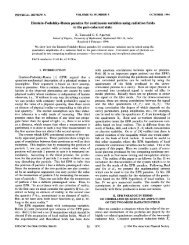
residuals. Fig. 4 shows a typical display of the weighted
residuals obtained by methods I and II in the analysis of
simulation data using Eq. (11) for excitation function
(cr = 0.2 ns, m = 1.2 ns, and W= 1 x 105), and Eq. (15)
for I(t) (AI = lO.O,T1 = 0.1 ns,A2 = 1,andT2 = 2ns). The
simulated excitation data, emission data, and fitted emission
data (method I) are shown in Fig. 4. In this case the
emission data was not normalized and the peak count
was -1.2 x I05. The distribution of the weighted residuals
in the region dominated by the short lifetime component is
more acceptable in Fig. 4 B than in Fig. 4 C. Deconvolution
by method I produced the following results: AI = 10.0,
Tr = 0.101 ns, A2 = 1.01, T2 = 2.00 ns, (reduced) chisquare
= 1.17, Durbin-Watson parameter (DWP) = 1.90,
standard normal variate of runs test (Z) = -0.05, and
percentage of weighted residuals between -2 and + 2
(PER) = 95.09. Deconvolution by method II produced the
following results: AI = 9.44, T1 = 0.106 ns, A2 = 1.01, T2 =
2.00 ns, chi-square = 1.41, DWP = 1.59, Z = 1.58, and
PER = 92.77.
In the simulations described earlier the time interval was
chosen to be 50 ps. The conclusion that the performance of
method I is better than method II when the short lifetime
in the decay equation is comparable to bt is independent of
the value of bt used in simulations. The computation time
required for method I or method II depends upon the
number of iterations required for convergence, which need
not be equal. On the average it is observed that method I
requires -10% more computer CPU time (Cyber 170/
730) than that required for method II. However, there
were several cases in which method I required less time
than method II because of convergence at a lower interation
number.
The method proposed here has also been used in the
analysis of experimental fluorescence data of standard
samples obtained by time-correlated single photon
counting technique. In comparison with the simulation
data the quality of the experimental data was poor because
of system errors, especially the wavelength response of the
photomultiplier which needed to be corrected in the analysis
by introducing a shift parameter. In spite of this, it is
generally observed that method I generates results with
BIOPHYSICAL JOURNAL VOLUME 54 1988

~~~~c
L 177 VIWSlKUw-UFLwV1i 1''9
Wo
Aol .I Aia Al.lr. /
(t)~ ~~
Lo
IAi,AhI
B
@~~~~~~~~~~~~~~
FIGURE 4. (A) Gaussian exccitation curve, simulated
| A ~~~~~~~~~~~~~~~~fluorescence decay curve for a two exponential decay
_ = ~~~~~~~~~~~~~~~~~~equation, and the smooth fluorescence decay curve
(S) -~~~~~~~~~~~ 1\\ ~~~~~~~obtained in fitting the emission data by method I. See
l e \ \ ~~~~~~~~~~~~~~~~~~~texct
for details. (B) Distribution of weighted residuals
0
obtained by method I and (C) by method II.
0-
on.00 2.50 5.00 7.50 10.00 12.50 15.00 17.50 20D.00
TIME (NS)
statistical test parameters that are marginally better than
those obtained by method II. It is not uncommon in the
analysis of experimental data to encounter a distribution of
residuals which appears bad only in the peak region in a
multiexponential fit of fluorescence decay. When all
instrument related errors are eliminated as a source of this
discrepancy, we suggest that one must also examine other
approximations for the numerical computation of Eq. (1).
CONCLUSION
In conclusion, use of recursion relations (Eqs. [5], [7], and
[8] is recommended in the deconvolution analysis of fluorescence
decay data by the nonlinear least-squares method
when a short lifetime component is suspected.
The author would like to thank Professor B. Venkataraman for a critical
reading of the manuscript.
Received for publication 10 March 1988 and in final form 31 May
1988.
REFERENCES
1. Bevington, P. R. 1960. In Data Reduction and Error Analysis for the
Physical Sciences. McGraw-Hill, Inc., New York.
2. Yguerabide, J., and E. Yguerabide, 1984. In Optical Techniques in
Biological Research. D. L. Rousseou, editor. Academic Press Inc.,
Orlando, FLA. 206-213
3. Grinvald, A., and I. Z. Steinberg. 1974. On the analysis of fluorescence
decay kinetics by the method of least-squares. Anal. Biochem.
59: 583-598.
4. O'Connor, D. V., and D. Phillips. 1984. In Time-Correlated Single
Photon Counting, Academic Press, Inc., London. 175.
5. Demas, J. N. 1983. In Excited State Lifetime Measurements.
Academic Press, Inc., New York. 209.
6. Van den Zegel, N. Boens, D. Daems, and F. C. De Schryver. 1986.
Possibilities and Limitations of the Time-Correlated Single Photon
Counting Technique: A comparative study of correction methods
for the wavelength dependence of the Instrument Response Function.
Chem. Phys. 101:311-335.
PERIASAMY Analysis ofFluorescence Decay 967