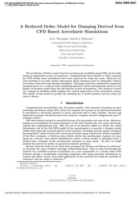
AIAA Paper 2006-2021 - CFD4Aircraft

47th AIAA/ASME/ASCE/AHS/ASC Structures, Structural Dynamics, and Materials Confere1 - 4 May 2006, Newport, Rhode IslandAIAA 2006-2021A Reduced Order Model for Damping Derived fromCFD Based Aeroelastic SimulationsM.A. Woodgate ∗ and K.J. Badcock † ,Computational Fluid Dynamics Laboratory,Flight Sciences and Technology,Department of Engineering,University of Liverpool,L69 3BX, United Kingdom.Keywords: CFD, computational aeroelasticityThe prediction of flutter onset based on aerodynamic modelling using CFD can be madeusing an augmented system of equations. Computational times similar to those requiredfor CFD steady state calculations have been reported for wing test cases. However, forsuch methods to be fully useful, information about damping must be obtainable withoutreverting to full order time domain simulation. This paper presents a method for computingdamping based on a reduced order modelling approach which systematically derives a twodegree of freedom model from the full discrete system of equations. The method is basedon a change of variables which employs the critical eigenvector of the aeroelastic system.The ability of this model to predict the damping for a model problem and two wing testcases is shown.I. IntroductionComputational aeroelasticity has developed rapidly, with attention focussing on timemarching calculations using CFD, where the response of a system to an initial perturbationis calculated to determine growth or decay, and from this to infer stability. Recent andimpressive example calculations have been made for complete aircraft configurations (see 123amongst others).The time domain method is powerful because of its generality and ease of use. However,basing an investigation of system dynamics in the time domain has one major drawback,namely the computational cost. This has led to an intensive effort to extract the usefulinformation out of the full CFD model of the aerodynamics to provide a cheaper modelwhich still retains the essential physics of the problem. Examples include proper orthognaldecomposition 4 which involves the extraction of modes using a limited set of time snapshotsof the flow evolution, a Volterra series which relates the aerodynamic response to someinput by a kernel 4 and system identification where a linear model is calculated from alimited time evolution of the aerodynamic response to some input. To date no singlemethod has proved its utility on general aeroelastic problems.Recent work has built on the ideas first presented by Morton and Beran in reference 5to calculate the onset of flutter through a Hopf Bifurcation. This is achieved through thesolution of a modified system of equations at a cost comparable to a steady state CFDsolution, giving a considerable advantage compared with using unsteady calculations tobracket the flutter speed. Successful application of the method was made for aerofoils inreference 9 and for wings in reference. 10∗ Research Assistant† Professor, corresponding author. Tel. : +44(0)151 794 4847 , Fax. : +44(0)151 794 6841, Email :K.J.Badcock@liverpool.ac.uk1 of 19American Institute of Aeronautics and AstronauticsCopyright © 2006 by K.J.Badcock and M.A.Woodgate. Published by the American Institute of Aeronautics and Astronautics, Inc., with permission.

Whilst knowledge of the onset of instability is important, other pieces of informationare required in practice. For example, flight tests measure damping and compare this withpredictions to inform decisions about future test points. If the stability boundary is to becrossed in flight then knowledge of the limit cycle oscillation amplitude is required. If thisrequires recourse to time domain simulations then much of the advantage of the methodsof the previous paragraph is lost. A systematic approach to model reduction is thereforerequired to supplement the rapid prediction of the flutter point.The perturbation method of multiple scales can be applied to determine behaviour closeto a bifurcation. This approach was used in 6 for a two dimensional aeroelastic problem andwas presented in 7 for the Duffing oscillator and in 8 for a three equation model problem.The idea is use a perturbation parameter ǫ to separate out events at different time scales.The terms of O(ǫ) provide a description of the linear dynamics of the system, and higherorder terms provide information about the effect of nonlinearities.The centre manifold theory provides a route to reducing a large dimension model toits essential dynamics. However, the practical obstacles to applying this approach to fullorder systems of more than 10 degrees of freedom have proved formidable. The currentpaper addresses this problem by using a change of coordinates for the system variableswhich allows the reduced model to be derived whilst preserving most of the structure ofthe original system, making manipulation of the reduction practical. Information from thedirect solution of the bifurcation point and its associated eigenvalue and eigenvectors 910 isused in this change of variables and the subsequent manipulation.The current paper adopts this approach to calculating a reduced order model. Furthersimplification of the approach is made for the prediction of damping and the method isassessed for a model problem followed by application to two flexible wings. The full centremanifold reduction is described in the appendix and is available for the model problembecause the second and third Jacobian matrices of the discrete operator, required forthe full centre manifold method but not for the simplified damping method, have beencalculated analytically. This task is much more difficult for the aeroelastic operator andso only the damping model has been used for the wings. The paper continues with theformulation of the reduced modelling, followed by a description of the full order systems.Results are then presented and evaluated, followed by conclusions.A. Stability CalculationConsider the nonlinear system of equationsII. Formulationẋ = f(x, µ), x ∈ R n (1)An equilibrium f(x 0, µ) = 0 experiences a loss of stability through a Hopf bifurcation forvalues of µ such that ∂f/∂x = A(x 0, µ) has a pair of eigenvalues ±iω which cross the imaginaryaxis. Denoting the corresponding eigenvector by q = q 1 + iq 2, the behaviour of the criticaleigenpair ω and q can be written asAq = iωq. (2)This equation can be written in terms of real and imaginary parts as Aq 1 + ωq 2 = 0 andAq 2 − ωq 1 = 0. A unique eigenvector is chosen by scaling against a constant real vector q sto produce a chosen complex value, taken to be 0 + 1i. This yields two additional scalarequations q T s q 1 = 0 and q T s q 2 − 1 = 0.A bifurcation point can be calculated directly by solving the augmented system of equationsf A(x A) = 0 (3)whereand x A = [x, q 1, q 2, µ, ω] T .⎡ ⎤fAq 1 + ωq 2f A =⎢ Aq 2 − ωq 1⎥⎣ qs T q 1⎦qs T q 2 − 1(4)2 of 19American Institute of Aeronautics and Astronautics

The bifurcation point can be calculated through a solution of equation 4 using Newton’smethod. This has been achieved for aerofoils free to move in pitch and plunge 9 and forflexible wings. 10 Full details of the calculation method are given in those references.B. Damping CalculationThe eigenvector which goes critical at a Hopf bifurcation will also be the least lightlydamped mode for parameter values in a region below the bifurcation value. In this regionthe aymptotic damping value will be determined by this mode. It is possible to reduce thefull system by a change of variables to calculate the damping by only considering a lowdimension reduced model. For aeroelastic systems we are dealing with systems of largedimension, and it is advantageous to use a change of variable which involves manipulatingthe system in its original form as far as possible. A summary of the general formulationbased on the centre manifold theory is given in the appendix. In this section a simplerversion of the general theory is given to allow damping to be calculated.The full system can be transformed by using only the vectors corresponding to thecritical eigenvalues of A and its transpose A T . These are calculated from equation 4. Thesystem is projected onto its critical eigenspace and complement. Suppose we have a Taylorexpansion of the residual function f about the equilibrium solution x 0 and parameter atthe bifurcation point µ 0, giving˙¯x = A¯x + F(¯x, ¯µ), x ∈ R n (5)where F(¯x, ¯µ) has at least quadratic terms and ¯x = x − x 0, ¯µ = µ − µ 0. The matrix A hasa pair of complex eigenvalues on the imaginary axis λ 1,2 = iω, ω > 0. Let q be the righteigenvector corresponding to λ 1. Then ¯q is the right eigenvector corresponding to λ 2 andAq = iωq,A¯q = −iω¯qThe left eigenvector p has the same propertyA T p = −iωp,A T ¯p = iω¯p.These can be normalised such that 〈p, q〉 = 1 where 〈p,q〉 = ∑ n¯piqi. The eigenspace Si=1corresponding to ±iω is two dimensional and is spanned by {Rq, Iq}. The eigenspace Tcorresponds to all the other eigenvalues of A and is n − 2 dimensional. Then y ∈ T if andonly if 〈p,y〉 = 0. Since y ∈ R n while p is complex then two real constraints on y exist andhence it is possible to decompose any ¯x ∈ R n as¯x = zq + ¯z¯q + ywhere z ∈ C 1 , zq + ¯z¯q ∈ S, and y ∈ T. The complex variable z is a coordinate of S so{z = 〈p, ¯x〉y = ¯x − 〈p, ¯x〉q − 〈¯p, ¯x〉¯qsince 〈p, ¯q〉 = 0. The equation (5) then has the form{ż = iωz + 〈p,F(zq + ¯z¯q + y, ¯µ)〉ẏ = Ay + F(zq + ¯z¯q + y, ¯µ) − 〈p,F(zq + ¯z¯q + y, ¯µ)〉q − 〈p, F(zq + ¯z¯q + y, ¯µ)〉¯qThis system is (n + 2) dimensional but we have two constraints on y.Now, in general at this stage a centre manifold reduction should be used to obtain arelationship between y and z which allows the critical dynamics to be calculated from thez equation only. This treatment allows nonlinear features such as Limit Cycle Oscillationsto be calculated from the reduced model. A description of the method to perform thisreduction is given in appendix A, and is referred to in the results section as the centremanifold reduced model. Here we are interested in calculating damping for parametervalues below the bifurcation point. In this case the influence of the component y from thenon-critical space is damped faster than the critical component z. We therefore neglectthe influence of y altogether which removes the need for the centre manifold reduction.Further justification for this approximation will be given from results for a test problembelow.3 of 19American Institute of Aeronautics and Astronautics

The damping is therefore determined by solving the equationż = iωz + 〈p, F(zq + ¯z¯q, ¯µ)〉 .This system is two dimensional. Finally, we need to calculate the form of F. Expandingthe function f in a Taylor series about the equilibrium solution x 0 and parameter µ 0 givesf(¯x, ¯µ) = f(x 0, µ 0) + ∂f∂x ¯x + 1 ∂ 2 f2 ∂x ¯x¯x + 1 ∂ 3 f2 6 ∂x ¯x¯x¯x + 3∂f∂µ ¯µ + 1 ∂ 2 f2 ∂µ 2 ¯µ2 + 1 ∂ 3 f6 ∂µ 3 ¯µ3 +∂ 2 f∂µ∂x ¯µ¯x + 1 ∂ 3 f2 ∂µ 2 ∂x ¯µ2¯x + 1 ∂ 3 f ¯µ¯x¯x + .....2 ∂µ∂x2 where all derivatives are evaluated at (x 0, µ 0). We can simplify this by noting that f(x 0, µ 0) =0 and neglecting terms which are quadratic and higher in ¯x and ¯µ. This leaveswhich means thatand hencef(¯x, ¯µ) ≈ A¯x + ∂f ∂A ¯µ +∂µ ∂µ ¯µ¯xF(¯x, ¯µ) = f µ¯µ + A µ¯µ¯x (6)〈p,F(zq + ¯z¯q, ¯µ)〉 = 〈p, f µ¯µ〉 + 〈p,A µ¯µ¯x〉.Using the change of coordinates and pulling the values of z and ¯z through the inner productwe obtain〈p, ¯µA µ¯x〉 = z〈p, ¯µA µq〉 + ¯z〈p, ¯µA µ¯q〉.This allows the reduced model to be written as a constant coefficient two degree of freedomsystem.This model is referred to in the results section as the damping reduced model. If theterm F is neglected altogether then we only retain linear terms, and this is referred to asthe linear reduced model. Further simplification of the damping reduced model is possiblefor the aeroelastic system and will be discussed below.To summarise, the damping calculation proceeds in the following steps:1. using the direct solver, calculate the Hopf bifurcation point and the critical eigenvalueand eigenvalue and the corresponding eigenvector of A T2. calculate the projected two degree of freedom model usingż = iωz + z〈p, ¯µA µq〉 + ¯z〈p, ¯µA µ¯q〉3. use the two degree of freedom model to compute the response of z to an initial disturbancefor values of µ < µ 0. This solution can be transformed back to the originalvariables using¯x = zq + ¯z¯qC. 2D non-adiabatic tubular reactor with axial mixingTo test the solution methodology for the augmented system, a model problem is consideredwhich describes the unsteady behaviour of a non-adiabatic tubular reactor with axialmixing, 1112∂y∂t∂Θ∂t==1 ∂ 2 yPe m ∂x − ∂y (Γ 2 ∂x − µy exp − Γ )Θ1 ∂ 2 ΘPe h ∂x − ∂Θ2 ∂x − β(Θ − ¯Θ) + µαy exp(Γ − Γ )Θwhere Pe m, Pe h , β, α, Γ, and ¯Θ are fixed constants and µ is the bifurcation parameter. Theboundary conditions (t > 0) are given by(7)∂y∂Θ= Pem(y − 1)∂x∂x= Pem(Θ − 1) (x = 0)4 of 19American Institute of Aeronautics and Astronautics

∂y∂x = ∂Θ = 0 (x = 1)∂xFor the results presented here the constants are set to Pe m = 5, Pe h = 5, β = 2.5, α = 0.5,Γ = 25, and ¯Θ = 1.0.The system is discretised using a cell centred finite difference scheme so that the firstand second differences are approximated by∣∂ 2 y ∣∣∣yi+1 − 2yi + yi−1=∂x 2 h 2i∂y ∣=∂x∣iyi+1 − yi−1.2hHere a uniform mesh of spacing h is used with the i-th point at x i = ih for (i = 0, . . . , n).The boundary conditions for x = 1 are applied by setting halo cell values to be identical tothe values in the adjacent interior cell.The solution for an equilibrium and also of the augmented system is by the full Newtonmethod with the use of the exact Jacobian on the left hand side. For the augmentedsystem, and the various types of reduced model, the first and second order Jacobian termshave been calculated analytically and were checked using finite differences. To check thereduced results, unsteady time stepping is also considered. An explicit method is usedwhich results in a large number of time steps (∆t = 1/500 is required for stability). Thebifurcation point is bracketed between a steady solution at one parameter value and anunsteady solution at a second value. Each new calculation halves the length of the regionbracketing the bifurcation value.D. 3D Aeroelastic System Based on the Euler EquationsThe three-dimensional Euler equations can be written in conservative form and Cartesiancoordinates as∂w f∂t+ ∂Fi∂x + ∂Gi∂y + ∂Hi∂z = 0 (8)where w f = (ρ,ρu, ρv, ρw,ρE) T denotes the vector of conserved variables. The flux vectorsF i , G i and H i are,⎛⎞ρU ∗ρuU ∗ + pF i =⎜ ρvU ∗⎟, (9)⎝ ρwU ∗ ⎠⎛G i =⎜⎝ρV ∗ρuV ∗ρvV ∗ + pρwV ∗V ∗ (ρE + p) + ẏU ∗ (ρE + p) + ẋ⎞ ⎛⎟H i =⎜⎠ ⎝ρW ∗ρuW ∗ρvW ∗ + pρwW ∗ + pW ∗ (ρE + p) + ż⎞⎟. (10)⎠In the above ρ, u, v, w p and E denote the density, the three Cartesian components of thevelocity, the pressure and the specific total energy respectively, and U ∗ , V ∗ , W ∗ the threeCartesian components of the velocity relative to the moving coordinate system which haslocal velocity components ẋ, ẏ and ż, i.e.The wing deflections δx s are defined at a set of points x s byU ∗ = u − ẋ (11)V ∗ = v − ẏ (12)W ∗ = w − ż (13)δx s = Σα iφ i (14)where φ i are the mode shapes calculated from a full finite element model of the structureand α i are the generalised coordinates. By projecting the finite element equations onto themode shapes the scalar equationsd 2 α idt 2 + ω2 i α i = µφ T i f s (15)5 of 19American Institute of Aeronautics and Astronautics

are obtained where f s is the vector of aerodynamic forces at the structural grid points, andµ = c 5 ρ ∞U 2 ∞. These equations are rewritten as a system in the formdw sdt= R s (16)where w s = (......, α i, α˙i, ....) T and R s = (......, α˙i, µφ T i f s − ωi 2 α i, ....) T .The aerodynamic forces are calculated at face centres on the aerodynamic surface gridand these must be transfered to the structural grid.. This problem was considered inreferences 13 and, 14 where a method was developed, called the constant volume tetrahedron(CVT) transformation. Denoting the fluid grid locations and aerodynamic forces as x a andf a, thenδx a = S(x a,x s, δx s)where S denotes the relationship defined by CVT. In practice this equation is linearised togiveδx a = S(x a,x s)δx sand then by the principle of virtual work, f s = S T f a.The grid speeds on the wing surface are also needed and these are approximated directlyfrom the linearised transformation asδx˙a = S(x a,x s)δẋ swhere the structural grid speeds are given byδx˙s = Σα˙iφ i. (17)We have to deal with the deforming geometry. This is achieved using Transfinite Interpolationof Displacements (TFI) within the blocks containing the wing. The wing surfacedeflections are interpolated to the volume grid points x ijk asδx ijk = ψ 0 j δx a,ik (18)where ψj 0 are values of a blending function 15 which varies between one at the wing surface(here j=1) and zero at the block face opposite. The surface deflections x a,ik are obtainedfrom the transformation of the deflections on the structural grid and so ultimately dependon the values of α i. The grid speeds can be obtained by differentiating equation (18) toobtain their explicit dependence on the values of α˙i.We will consider the bifurcation parameter as µ. For symmetric wings at zero incidenceany equilibrium solution has the wing undeflected. This means that f s = 0 at the equilibriumsolution. The fluid equations do not depend explicitly on µ. Therefore f µ = 0 in equation4 for an equilibrium solution. Also, the linear dependence of the structural equations onµ means that A µ is constant and only has non zero terms in the small number of rowscorresponding to the structural equations.A. Tubular ReactorIII. ResultsThe rich solution space for this model problem is shown in figure 1. This includes stableand unstable equilibria, limit points and Hopf bifurcation points. There is also a hysteresisloop for increasing and decreasing µ. The solution is characterised by the maximum valueof Θ within the domain. The equilibrium solutions for varying µ are shown in figure 1.For µ < 0.165 and µ > 0.180 this equilibrium is stable and the solution to equation (7)is steady. For 0.165 < µ < 0.180 the equilibrium is unstable and a limit cycle oscillation isformed. Depending on whether the parameter µ is increased (solid line) or decreased (solidswitching to dashed lines with increasing µ) a different equilibrium is obtained, indicatinghysteresis. The equilibria were mapped out using a continuation method with Newton’smethod for the corrector stage. In addition, time marching calculations were done to mapout the stability of these equilibria.Next, the augmented system (equation 3) was solved to find the bifurcation points.If the initial guess is poor then the solution diverges. For the current calculations thefollowing initial guess was used: µ = 0.16, x 2i = 1.0, x 2i+1 = 0.0, P 1i = √ n1, P 22i = √ n1,6 of 19American Institute of Aeronautics and Astronautics

1.26Maximum value of Theta in [0,1]1.241.221.21.181.161.141.121.11.08forwardsbackwards1.060.15 0.155 0.16 0.165 0.17 0.175 0.18 0.185 0.19Bifurcation ParameterFigure 1. The equilibrium solution as mapped out by a continuation method varing the bifurcation parameterµP 22i+1 = − √ n1, q = P 2 and the eigenvalue i. By changing the initial conditions the Newtoniterations can be made to converge to the second Hopf point at µ = 0.180. Starting from thisguess the iterations had to be under-relaxed by a factor 0.5 until the domain of quadraticconvergence was reached (the criteria used was based on the initial residual being reducedby half). A sequence of grids was used to show mesh independence and a second methodof initialisation was used by taking the final solution from the previous grid in the sequenceas the starting solution on the next grid. No relaxation was required using this technique.Damping calculations were made using the reduced model. Various results are comparedto gain some insight into the behaviour of the different options. The benchmark is the timedomain solution of the full system, which is indicated by the dots on the time responsecurves. Secondly, the full centre manifold reduction is based on the Taylor expansion ofthe residual including third order terms, and using the reduction methodology describedin the appendix. Finally, the key results are obtained using the simpler damping reductionusing the Tayor expansion of equation 6.We consider results about the bifurcation point µ 0 = 0.16508 and for values of ¯µ of -0.00005, -0.0001 and -0.0002. Although it is beyond the scope of this paper, results arealso shown in figure 2 for ¯µ = 0.00007 which results in a limit cycle. The centre manifoldreduction predicts the LCO response perfectly.The damped responses for ¯µ = −0.00005, ¯µ = −0.0001 and ¯µ = −0.0002 are shown in figure3. The centre manifold results, which arise from solving a two degrees of freedom system,agree perfectly with the full order (here 512 degrees of freedom) system results for allthree cases. Finally, the damping reduced model predicts the response very well. Giventhe relative simplicity of calculating the damping reduced model, these results suggest astrong preference for this approach.B. AGARD 445.6 WingThe behaviour of the method is next investigated for the aeroelastic response of theAGARD 445.6 wing. Time domain and bifurcation results are given in. 10 The grid has17900 points and is optimised to have a large number of points in the tip region which iscritical for predicting flutter onset. The four important modes from the structural model,which is of the plate variety, were retained. The flutter boundary is shown in figure 4, withbelow the curve being the stable region.Second and Third Jacobians of the full CFD operator proved unreliable from finite7 of 19American Institute of Aeronautics and Astronautics

y(1)0.070.060.050.040.030.020.010-0.01-0.02-0.03-0.04-0.05-0.06-0.07-0.080 50 100 150TimeFull Systemlinear termsfull centre manifoldFigure 2. Comparison of results from the full model, centre manifold reduced model and linear reduced modelfor an LCO response at ¯µ = 0.000078 of 19American Institute of Aeronautics and Astronautics

0.0040.00350.0030.0080.0070.006y(1)0.00250.002y(1)0.0050.0040.00150.0010.00050Full Systemdamping termsfull centre manifold0 100 200 300 400Time0.0030.0020.00100 100 200TimeFull Systemdamping termsfull centre manifold(a) ¯µ = −0.00005 (b) ¯µ = −0.00010.0180.0160.0140.012y(1)0.010.0080.0060.004Full Systemdamping termsfull centre manifold0.0020 50 100Time(c) ¯µ = −0.0002Figure 3. Comparison of results from the full model, centre manifold reduced model, damping reduced modeland linear reduced model for damped responses at ¯µ = −0.00005, ¯µ = −0.0001 and ¯µ = −0.0002.9 of 19American Institute of Aeronautics and Astronautics

difference calculations and remedies to this were left to future work. Therefore the centremanifold reduced model was unavailable for the aeroelastic cases.The reduced damping model predictions were calculated for values of dynamic pressurewhich are 5%,10%,20% and 40% below the bifurcation value for Mach numbers of 0.67, 0.90,0.96 and 1.07. The reduced model (two degrees of freedom) responses are compared withthe full order system (89508 degrees of freedom) in figures 5 - 8. A number of commentscan be made. First, as the dynamic pressure tends to the flutter value, the reduced modelpredictions converge to those of the full model as expected. The more heavily dampedresults at M=0.67 show more discrepancy than the other three cases, which show goodagreement, even at 60 % of the flutter value. It is possible that the addition of higherorder terms from the centre manifold reduction may allow improved prediction for theheavily damped cases and this will be investigated in future work. The typical CPU timefor a full order time domain calculation is 142 times a steady state calculation. The reducedmodel takes a negligible time to run, and is formed (once only for each Mach number) ata cost comparable to 3.2 steady state calculations. Once formed the responses can beapproximated almost free for any value of the dynamic pressure below the critical value.650060005500Dynamic Pressure50004500400035003000250020000.7 0.8 0.9 1 1.1MachFigure 4. Flutter boundary for AGARD wing traced out using the bifurcation solver.C. Hawk WingFinally, we present results representing the wing of the Hawk trainer which is manufacturedby BAE SYSTEMS. A previous study of the flutter characteristics of this aircraft wasreported in reference 3 using the time domain approach. Predictions for several models ofthe Hawk were compared, including a linear method, a CFD based model of the wingbody-tailplane,and the wing alone.In the current calculations an aerodynamic grid with 16644 points was generated whichwas found to give reliable results in the previous paper through a grid refinement study.10 of 19American Institute of Aeronautics and Astronautics

0.0010.0010.000750.000750.00050.0005displacement0.000250-0.00025fullreduceddisplacement0.000250-0.00025fullreduced-0.0005-0.0005-0.00075-0.00075-0.0010 50 100 150 200Time-0.0010 50 100 150 200Time(a) 60% (b) 80%0.0010.001250.000750.0010.00050.00075displacement0.000250-0.00025fullreduceddisplacement0.00050.000250-0.00025fullreduced-0.0005-0.0005-0.00075-0.00075-0.001-0.0010 50 100 150 200Time-0.001250 50 100 150 200 250Time(c) 90% (d) 95%Figure 5. Comparison of results from the full model and damping reduced model at M=0.67 for values ofdynamic pressure below the flutter boundary.11 of 19American Institute of Aeronautics and Astronautics

0.0010.0010.000750.000750.00050.0005displacement0.000250-0.00025fullreduceddisplacement0.000250-0.00025fullreduced-0.0005-0.0005-0.00075-0.00075-0.0010 50 100 150 200Time-0.0010 50 100 150 200Time(a) 60% (b) 80%0.0010.0010.000750.000750.00050.0005displacement0.000250-0.00025fullreduceddisplacement0.000250-0.00025fullreduced-0.0005-0.0005-0.00075-0.00075-0.0010 50 100 150 200Time-0.0010 50 100 150 200Time(c) 90% (d) 95%Figure 6. Comparison of results from the full model and damping reduced model at M=0.90 for values ofdynamic pressure below the flutter boundary.12 of 19American Institute of Aeronautics and Astronautics

0.0010.0010.000750.000750.00050.0005displacement0.000250-0.00025fullreduceddisplacement0.000250-0.00025fullreduced-0.0005-0.0005-0.00075-0.00075-0.0010 50 100 150 200Time-0.0010 50 100 150 200Time(a) 60% (b) 80%0.0010.0010.000750.000750.00050.0005displacement0.000250-0.00025fullreduceddisplacement0.000250-0.00025fullreduced-0.0005-0.0005-0.00075-0.00075-0.0010 50 100 150 200Time-0.0010 50 100 150 200Time(c) 90% (d) 95%Figure 7. Comparison of results from the full model and damping reduced model at M=0.96 for values ofdynamic pressure below the flutter boundary.13 of 19American Institute of Aeronautics and Astronautics

0.0010.0010.000750.000750.00050.0005displacement0.000250-0.00025fullreduceddisplacement0.000250-0.00025fullreduced-0.0005-0.0005-0.00075-0.00075-0.0010 50 100 150 200Time-0.0010 50 100 150 200Time(a) 60% (b) 80%0.0010.0010.000750.000750.00050.0005displacement0.000250-0.00025fullreduceddisplacement0.000250-0.00025fullreduced-0.0005-0.0005-0.00075-0.00075-0.0010 50 100 150 200Time-0.0010 50 100 150 200Time(c) 90% (d) 95%Figure 8. Comparison of results from the full model and damping reduced model at M=1.07 for values ofdynamic pressure below the flutter boundary.14 of 19American Institute of Aeronautics and Astronautics

The structural dynamics is represented by a beam model, supplied by BAE SYSTEMS.A full description of how the transformation is done from this structural model is givenin reference. 3 The four lowest frequency symmetric non-tailplane modes in the structuralmodel are retained for the flutter calculations. These have frequencies 12.42Hz (1st wingbending), 14.43Hz (the influence of the 1st fuselage bending mode on the wing), 32.46Hz(the influence of the 2nd fuselage bending mode on the wing) and 37.87Hz (the first wingtorsion mode). In the linear aeroelastic predictions made with the same four modes, thefirst wing bending and torsion modes couple, the other two modes having only a smallinfluence on the flutter mechanism. This structural model provided an ideal test case forthe CFD based methods. The full aero-structural model has 16652 degrees of freedom.The bifurcation solver was first used to trace out the flutter boundary which is shown infigure 9. The prediction of damping was then evaluated for the Mach number which resultsin the lowest point on the transonic flutter dip. Values of dynamic pressure at 98%, 95%and 92% of the critical value were chosen. Even at 98% of the critical value the dampingis heavy, in contrast with the AGARD wing for the Mach number in the flutter dip.The comparison between the damping reduced model and the full order model is shownin figure 10. The agreement at 98 % of the critical value is close and in terms of dampingthe reduced model predictions are not too disimilar at 95% and 92% either. However, closeinspection of the comparisons shows that the frequencies of the responses at the lower twovalues are significantly in disagreement. Calculation of the eigenspectrum by the inversepower method shows that the closest mode to the imaginary axis is the critical mode onlyafter the bifurcation parameter is 96% of the critical value. Below this a lower frequencymode dominates the response.The time domain calculation of the full order system in this cases took in excess of 10hours on a Pentium 4 processor. The reduced model took less than 20 seconds to computethe same case.IV. ConclusionsPrevious work has shown that the flutter onset speed can be computed for CFD-CSDcoupled models using fast methods based on the behaviour of the critical eigenvalue. Flutterspeeds can be computed in roughly the cost of a steady state calculation, avoiding the largecosts associated with time domain analysis.In the current paper a method which uses information available about the critical eigenvectorof the system has been presented which forms a two-degree-of-freedom model tocompute the damped response at values of the dynamic pressure below the critical value.This information has the potential to allow rapid evaluation of damping characteristicsprior to flight testing.Results were shown for a Tubular Reactor model problem and then for the aeroelasticbehaviour of the AGARD and Hawk wings. Close to the critical parameter value the fullorder system response is reproduced well by the two degree of freedom model. As theresponse becomes more heavily damped the agreement becomes less good, but these casesare also less critical in the real situation.Results using a centre manifold correction were presented for the Tubular Reactormodel problem and excellent agreement was obtained with the full order system, even forheavily damped conditions. Further work is underway to accurately evaluate the secondand third Jacobians of the aeroelastic operator to allow this correction to be applied forthe aeroelastic cases. In addition, and most interestingly, this will allow post-bifurcationbehaviour (i.e. LCO’s) to be computed also.V. AcknowledgementsThis work was supported by BAE SYSTEMS, Engineering and Physical Sciences ReserachCouncil and Ministry of Defence, and is part of the work programme of the Partnershipfor Unsteady Methods in Aerodynamics (PUMA) Defence and Aerospace Research Partnership(DARP).15 of 19American Institute of Aeronautics and Astronautics

Figure 9. Flutter boundary for Hawk wing traced out using the bifurcation solver. The values of dynamicpressure at which the damping model is compared with full order results are indicated by the dots.16 of 19American Institute of Aeronautics and Astronautics

(a) 92% (b) 95%(c) 98%Figure 10. Comparison of results from the full model and damping reduced model for the Hawk wing in thetransonic dip and for values of dynamic pressure below the flutter boundary.17 of 19American Institute of Aeronautics and Astronautics

References1 Farhat, C, Geuzaine, P and Brown. G, Application of a three-field nonlinear fluid-structureformulation to the prediction of the aeroelastic parameters of an F-16 fighter, Computers andFluids, to appear, 2002.2 Melville, R, Nonlinear Simulation of F-16 Aeroelastic Instability, AIAA Paper 2001-0570,January, 2001.3 Woodgate, M.A., Badcock, K.J., Rampurawala, A.M., Richards, B.E., Nardini, D. and Henshaw,M, Aeroelastic Calculations for the Hawk Aircraft Using the Euler Equations, Journal ofAircraft,42 (4), 1005-1012, 2005.4 Lucia, D.J., Beran, P.S. and Silva, W.A, Reduced-order modeling: new approaches for computationalphysics, Progress in Aerospace Sciences, 40(1-2), 51-117, 2004.5 Morton, S.A. and Beran, P.S., Hopf-Bifurcation Analysis of Airfoil Flutter at Transonic Speeds, JAircraft, 36, pp 421-429, 1999.6 Beran, P.S., Computation of a Limit-Cycle Oscillation using a Direct Method, AIAA Paper.7 Nayfeh, A.H. and Balachandran, B., Applied Nonlinear Dynamics, Wiley, New York, 1995.8 Nayfeh, A.H. and Balachandran, B., Motion near a Hopf bifurcation of a three-dimensionalsystem, Mech Res Comm, 17, 191-198, 1990.9 Badcock, K.J., M.A. Woodgate, M.A. and Richards, B.E., The Application of Sparse MatrixTechniques for the CFD based Aeroelastic Bifurcation Analysis of a Symmetric Aerofoil, AIAA J,42(5) 883-892, May, 2004.10 Badcock, K.J., Woodgate, M.A. and Richards, B.E., Direct Aeroelastic Bifurcation Analysisof a Symmetric Wing Based on the Euler Equations, Journal of Aircraft, 42(3),731-737, 2005.11 Ortiz,E.L., Step by step Tau method, Comput. Math Appl, 1, pp 381-392 1975.12 Beran, P.S. and Carlson, C.D., Domain-decomposition methods for Bifurcation Analysis,AIAA Paper 97-0518, 1997.13 Goura, G.S.L., Time Marching Analysis of Flutter using Computational Fluid Dynamics, PhDthesis, University of Glasgow, Nov, 2001.14 Goura, G.S.L., Badcock, K.J., Woodgate, M.A. and Richards, B.E., Extrapolation Effects onCoupled CFD-CSD Simulations, AIAA J, Vol 41(2), 312-314, 2003.15 Gordon, W.J. and Hall, C.A., Construction of curvilinear coordinate systems and applicationsto mesh generation, Int J Num Meth Engr, 7, 1973, 461-477.A. Classical Model ReductionConsider the nonlinear system of equationsẋ = f(x), x ∈ R n (19)where f is sufficiently smooth. We assume that we are at a Hopf bifurcation and hencethe Jacobian matrix ∂f/∂x has 2 and only 2 critical eigenvalues with zero real part and theremaining m = n − 2 eigenvalues have negative real parts. Then the system (19) can betransformed to {˙u = Bu + g(u, v)(20)˙v = Cv + h(u, v)where u ∈ R 2 and v ∈ R m . B is a 2 ×2 matrix with its eigenvalues on the imaginary axis andC is a m × m matrix with no eigenvalues on the imaginary axis. The functions g and h haveat least quadratic terms. The centre manifold W c of system (20) can be locally representedas a graph of a smooth function,W c = {(u, v) : v = V (u)} (21)V : R 2 → R m and due to the tangent property of W c , V (u) = O(||u|| 2 ).The Reduction Principle says system (20) is locally topologically equivalent near theorigin to{˙u = Bu + g(u,V (u))(22)˙v = CvThe important thing to notice is that the equations for u and v are decoupled in equation(22). The first equation is the restriction of equation (20) to its centre manifold. Thedynamics of the structurally unstable system (20) are essentially determined by this restriction,since the second equation in (22) is linear. For a Hopf bifurcation with (λ 1,2 = ±iω)then the system looks like⎧ ( ) ( )( ) ( )⎨ u1 ˙ 0 −ω u1 G1(u 1, u 2, v)=+u˙⎩2 ω 0 u 2 G 2(u 1, u 2, v)(23)˙v = Cv + H 1(u 1, u 2, v)18 of 19American Institute of Aeronautics and Astronautics

It is possible to rewrite this in complex form by use of the variable z = u 1 + iu 2 to obtain{ż = iωz + G(z, ¯z, v)˙v = Cv + H(z, ¯z, v)(24)where G and H are smooth complex-valued functions of z, ¯z ∈ C 1 of at least quadratic order.The centre manifold W c can be locally represented as a graph of a smooth functionW c = {(z, v) : v = V (z)}V maps R 2 → R n−2 and due to the tangent property of W c , V (z) = O||u|| 2 . The Centremanifold W c therefore has the representationv = V (z, ¯z) = 1 2 w20z2 + w 11z¯z + 1 2 w02¯z2 + O(|z| 3 ), (25)with the coefficients w ij ∈ C 2 . Since v must be real, w 11 is real and w 20 = ¯w 02. Using Taylorexpansions in z, ¯z, and v the system (24) can be rewritten as⎧⎨⎩ż = iωz + 1 2 G20z2 + G 11z¯z + 1 2 G02¯z2+ 1 G21z2¯z + 〈G2 10, v〉z + 〈G 01, v〉¯z + . . .˙v = Cv + 1 2 H20z2 + H 11z¯z + 1 2 H02¯z2 + . . .where G 20, G 11, G 02, G 21 ∈ C 1 and G 01, G 10, H ij ∈ C n−2 . Since v is real H 11 is real, andH 20 = ¯H 02.G jk =∂j+k∂z j ∂¯z k G(z, ¯z,0) ∣ ∣∣∣z=0(26), j + k ≥ 2, (27)Ḡ 10,j =Ḡ 01,j =∂2∂v j∂z G(z, ¯z, v) ∣ ∣∣∣z=0,v=0∂2∂v j∂¯z G(z, ¯z, v) ∣ ∣∣∣z=0,v=0, j = 1,2, . . . , n − 2, (28), j = 1,2, . . . , n − 2, (29)∂j+k∣ ∣∣∣H jk =∂z j ∂¯z H(z, ¯z, 0) , j + k = 2, (30)kz=0On substituting the representation of the centre manifold in (26) and equating coeffients,w 20 = (2iωI − C) −1 H 20w 11 = −C −1 H 11(31)w 02 = (−2iωI − C) −1 H 20Where I is the identity matrix and the matrices (2iωI −C), C and (−2iωI −C) are invertiblesince 0 and ±2iω are not eigenvalues of C.For reduction to be worthwhile the bifurcation parameter must also be added to thesystem and included in the calculated centre manifolds. This allows the reduced model to beapplied for parameter values away from the bifurcation value. Consider the parameterizedequationẋ = F(x,α)where x ∈ R n and α ∈ R m . Suppose that at α = 0 the system has a non-hyperbolic equilibriumx = 0 which undergoes a Hopf bifurcation. This means we have a system equivalentto {˙u = Bu + g(u,v, α)(32)˙v = Cv + h(u, v, α)and since α does not depend on time we can append the equation ˙α = 0 to the expandedsystem⎧⎨ ˙u = Bu + g(u,v, α)˙v = Cv + h(u, v, α)(33)⎩˙α = 0The Centre Manifold theorem asserts the existence of a centre manifold for the origin thatis local given by points (u, v, α) satisfying an equation of the formThis is used in the reduction step.v = k(u, α).19 of 19American Institute of Aeronautics and Astronautics