Advanced Quantum Field Theory

Advanced Quantum Field TheoryRoberto CasalbuoniDipartimento di FisicaUniversita di FirenzeLectures given at the Florence University during the academic year 1998/99.

ContentsIndex . . . . . . . . . . . . . . . . . . . . . . . . . . . . . . . . . . . . . . 11 Notations and Conventions 41.1 Units . . . . . . . . . . . . . . . . . . . . . . . . . . . . . . . . . . . . 41.2 Relativity and Tensors . . . . . . . . . . . . . . . . . . . . . . . . . . 61.3 The Noether's theorem for relativistic elds . . . . . . . . . . . . . . 61.4 Field Quantization . . . . . . . . . . . . . . . . . . . . . . . . . . . . 91.4.1 The Real Scalar Field . . . . . . . . . . . . . . . . . . . . . . . 101.4.2 The Charged Scalar Field . . . . . . . . . . . . . . . . . . . . 121.4.3 The Dirac Field . . . . . . . . . . . . . . . . . . . . . . . . . . 141.4.4 The Electromagnetic Field . . . . . . . . . . . . . . . . . . . . 171.5 Perturbation Theory . . . . . . . . . . . . . . . . . . . . . . . . . . . 271.5.1 The Scattering Matrix . . . . . . . . . . . . . . . . . . . . . . 271.5.2 Wick's theorem . . . . . . . . . . . . . . . . . . . . . . . . . . 291.5.3 Feynman diagrams in momentum space . . . . . . . . . . . . . 301.5.4 The cross-section . . . . . . . . . . . . . . . . . . . . . . . . . 332 One-loop renormalization 362.1 Divergences of the Feynman integrals . . . . . . . . . . . . . . . . . . 362.2 Higher order corrections . . . . . . . . . . . . . . . . . . . . . . . . . 382.3 The analysis by counterterms . . . . . . . . . . . . . . . . . . . . . . 452.4 Dimensional regularization of the Feynman integrals . . . . . . . . . . 522.5 Integration in arbitrary dimensions . . . . . . . . . . . . . . . . . . . 542.6 One loop regularization of QED . . . . . . . . . . . . . . . . . . . . . 562.7 One loop renormalization . . . . . . . . . . . . . . . . . . . . . . . . . 633 Vacuum expectation values and the S matrix 733.1 In- and Out-states . . . . . . . . . . . . . . . . . . . . . . . . . . . . 733.2 The S matrix . . . . . . . . . . . . . . . . . . . . . . . . . . . . . . . 793.3 The reduction formalism . . . . . . . . . . . . . . . . . . . . . . . . . 814 Path integral formulation of quantum mechanics 854.1 Feynman's formulation of quantum mechanics . . . . . . . . . . . . . 854.2 Path integral in conguration space . . . . . . . . . . . . . . . . . . . 881

4.3 The physical interpretation of the path integral . . . . . . . . . . . . 914.4 The free particle . . . . . . . . . . . . . . . . . . . . . . . . . . . . . 974.5 The case of a quadratic action . . . . . . . . . . . . . . . . . . . . . . 994.6 Functional formalism . . . . . . . . . . . . . . . . . . . . . . . . . . . 1044.7 General properties of the path integral . . . . . . . . . . . . . . . . . 1074.8 The generating functional of the Green's functions . . . . . . . . . . . 1134.9 The Green's functions for the harmonic oscillator . . . . . . . . . . . 1165 The path integral in eld theory 1235.1 The path integral for a free scalar eld . . . . . . . . . . . . . . . . . 1235.2 The generating functional of the connected Green's functions . . . . . 1275.3 The perturbative expansion for the theory ' 4 . . . . . . . . . . . . . 1295.4 The Feynman's rules in momentum space . . . . . . . . . . . . . . . . 1355.5 Power counting in ' 4 . . . . . . . . . . . . . . . . . . . . . . . . . . 1375.6 Regularization in ' 4 . . . . . . . . . . . . . . . . . . . . . . . . . . . 1425.7 Renormalization in the theory ' 4 . . . . . . . . . . . . . . . . . . . 1456 The renormalization group 1526.1 The renormalization group equations . . . . . . . . . . . . . . . . . . 1526.2 Renormalization conditions . . . . . . . . . . . . . . . . . . . . . . . . 1566.3 Application to QED . . . . . . . . . . . . . . . . . . . . . . . . . . . 1606.4 Properties of the renormalization group equations . . . . . . . . . . . 1616.5 The coecients of the renormalization group equations and the renormalizationconditions . . . . . . . . . . . . . . . . . . . . . . . . . . . 1677 The path integral for Fermi elds 1697.1 Fermionic oscillators and Grassmann algebras . . . . . . . . . . . . . 1697.2 Integration over Grassmann variables . . . . . . . . . . . . . . . . . . 1747.3 The path integral for the fermionic theories . . . . . . . . . . . . . . . 1788 The quantization of the gauge elds 1808.1 QED as a gauge theory . . . . . . . . . . . . . . . . . . . . . . . . . . 1808.2 Non-abelian gauge theories . . . . . . . . . . . . . . . . . . . . . . . . 1828.3 Path integral quantization of the gauge theories . . . . . . . . . . . . 1868.4 Path integral quantization of QED . . . . . . . . . . . . . . . . . . . 1968.5 Path integral quantization of the non-abelian gauge theories . . . . . 2008.6 The -function in non-abelian gauge theories . . . . . . . . . . . . . . 2049 Spontaneous symmetry breaking 2139.1 The linear -model . . . . . . . . . . . . . . . . . . . . . . . . . . . . 2139.2 Spontaneous symmetry breaking . . . . . . . . . . . . . . . . . . . . . 2199.3 The Goldstone theorem . . . . . . . . . . . . . . . . . . . . . . . . . . 2239.4 The Higgs mechanism . . . . . . . . . . . . . . . . . . . . . . . . . . 2259.5 Quantization of a spontaneously broken gauge theory in the R -gauge 2302

9.6 -cancellation in perturbation theory . . . . . . . . . . . . . . . . . . 23510 The Standard model of the electroweak interactions 23910.1 The Standard Model of the electroweak interactions . . . . . . . . . . 23910.2 The Higgs sector in the Standard Model . . . . . . . . . . . . . . . . 24410.3 The electroweak interactions of quarks and the Kobayashi-Maskawa-Cabibbo matrix . . . . . . . . . . . . . . . . . . . . . . . . . . . . . . 24910.4 The parameters of the SM . . . . . . . . . . . . . . . . . . . . . . . . 257A 259A.1 Properties of the real antisymmetric matrices . . . . . . . . . . . . . 2593

Chapter 1Notations and Conventions1.1 UnitsIn quantum relativistic theories the two fundamental constants c e h/, the lightvelocity and the Planck constant respectively, appear everywhere. Therefore it isconvenient to choose a unit system where their numerical value is given byc = h/ =1 (1.1)For the electromagnetism we will use the Heaviside-Lorentz system, where we takealso 0 =1 (1.2)From the relation 0 0 =1=c 2 it followsIn these units the Coulomb force is given byj ~Fj = e 1e 24 0 =1 (1.3)1j~x 1 ; ~x 2 j 2 (1.4)and the Maxwell equations appear without any visible constant. For instance thegauss law is~r ~E = (1.5)dove is the charge density. The dimensionless ne structure constant =e24 0 h/c(1.6)is given by = e24(1.7)4

Any physical quantity can be expressed equivalently by using as fundamentalunit energy, mass, lenght or time in an equivalent fashion. In fact from our choicethe following equivalence relations followct ` =) time lenghtE mc 2 =) energy massE pv =) energy momentumEt h/ =) energy (time) ;1 (lenght) ;1 (1.8)In practice, it is enough to notice that the product ch/ has dimensions [E`]. ThereforeRecalling thatit followsFrom whichch/ =3 10 8 mt sec ;1 1:05 10 ;34 J sec = 3:15 10 ;26 J mt (1.9)ch/ =1eV=e 1=1:602 10 ;19 J (1.10)3:15 10;261:6 10 ;13 MeV mt =197MeV fermi (1.11)1MeV ;1 = 197 fermi (1.12)Using this relation we can easily convert a quantity given in MeV (the typical unitused in elementary particle physics) in fermi. For instance, using the fact that alsothe elementary particle masses are usually given in MeV , the wave lenght of anelectron is given by e Compton= 1 m e10:5 MeV200 MeV fermi0:5 MeV 400 fermi (1.13)Therefore the approximate relation to keep in mind is 1 = 200 MeV fermi. Furthermore,usingc =3 10 23 fermi sec ;1 (1.14)we getandAlso, usingit follows from (1.12)1 fermi = 3:3 10 ;24 sec (1.15)1MeV ;1 =6:58 10 ;22 sec (1.16)1 barn = 10 ;24 cm 2 (1.17)1GeV ;2 =0:389 mbarn (1.18)5

1.2 Relativity and TensorsOur conventions are as follows: the metric tensor g is diagonal with eigenvalues(+1 ;1 ;1 ;1). The position and momentum four-vectors are given byx =(t ~x) p =(E~p) =0 1 2 3 (1.19)where ~x and ~p are the three-dimensional position and momentum. The scalar productbetween two four-vectors is given bywhere the indices have been lowered bya b = a b g = a b = a b = a 0 b 0 ; ~a ~ b (1.20)a = g a (1.21)and can be raised by using the inverse metric tensor g g . The four-gradientis dened as @ =@ @@x = @t @= @ t ~r (1.22)@~xThe four-momentum operator in position space isThe following relations will be usefulp ! i @@x =(i@ t ;i~r) (1.23)p 2 = p p !; @ @= ; (1.24)@x @x x p = Et ; ~p ~x (1.25)1.3 The Noether's theorem for relativistic eldsWe will now review the Noether's theorem. This allows to relate symmetries of theaction with conserved quantities. More precisely, given a transformation involvingboth the elds and the coordinates, if it happens that the action is invariant underthis transformation, then a conservation law follows. When the transformationsare limited to the elds one speaks about internal transformations. When bothtypes of transformations are involved the total variation of a local quantity F (x)(that is a function of the space-time point) is given byF (x)= ~F (x 0 ) ; F (x) = ~F (x + x) ; F (x) = ~F (x) ; F (x)+x @F(x)@x (1.26)6

The total variation keeps into account both the variation of the reference frameand the form variation of F . It is then convenient to dene a local variation F,depending only on the form variationThen we getF(x) = ~F (x) ; F (x) (1.27)F (x) =F(x)+x @F(x)(1.28)@x Let us now start form a generic four-dimensional actionS =ZVd 4 x L( i x) i =1:::N (1.29)and let us consider a generic variation of the elds and of the coordinates, x 0 =x + x i (x) = ~ i (x 0 ) ; i (x) i (x)+x @@x (1.30)If the action is invariant under the transformation, thenThis gives rise to the conservation equation~S V 0 = S V (1.31)@ Lx + @L i ; x @L i@ i @ i =0 (1.32)This is the general result expressing the local conservation of the quantity in parenthesis.According to the choice one does for the variations x and i , and ofthe corresponding symmetries of the action, one gets dierent kind of conservedquantities.Let us start with an action invariant under space and time translations. In thecase we take x = a with a independent onx e i =0. From the general resultin eq. (1.32) we get the following local conservation lawT = @L i@ i ;Lg @ T =0 (1.33)T is called the energy-momentum tensor of the system. From its local conservationwe get four constant of motionP =Zd 3 xT 0 (1.34)P is the four-momentum of the system. In the case of internal symmetries we takex =0. The conserved current will beJ = @L i = @L i @@ i @ i J =0 (1.35)7

with an associated constant of motion given byQ =Zd 3 xJ 0 (1.36)In general, if the system has more that one internal symmetry, we may have morethat one conserved charge Q, thatis we have a conserved charge for any .The last case we will consider is the invariance with respect to Lorentz transformations.Let us recall that they are dened as the transformations leaving invariantthe norm of a four-vectorx 2 = x 0 2(1.37)For an innitesimal transformationwithx 0 = x x + x (1.38) = ; (1.39)We see that the number of independent parameters characterizing a Lorentz transformationis six. As well known, three of them correspond to spatial rotations,whereas the remaining three correspond to Lorentz boosts. In general, the relativisticelds are chosen to belong to a representation of the Lorentz group ( for instancethe Klein-Gordon eld belongs to the scalar representation). This means that undera Lorentz transformation the components of the eld mix together, as, for instance,a vector eld does under rotations. Therefore, the transformation law of the elds i under an innitesimal Lorentz transformation can be written as i = ; 1 2 ij j (1.40)where we have required that the transformation of the elds is of rst order in theLorentz parameters . The coecients (antisymmetric in the indices ( ))dene a matrix in the indices (i j) which can be shown to be the representative ofthe innitesimal generators of the Lorentz group in the eld representation. Usingthis equation and the expression for x we get the local conservation law @L0 = @ i@ i ;Lg x + 1 2@L@ i = 1 ;T 2 @L@ x ; T x + ij@ j i and dening (watch at the change of sign) ij j (1.41)M = x T ; x T ; @L ij@ j (1.42)i 8

it follows the existence of six locally conserved currents (one for each Lorentz transformation)@ M =0 (1.43)and consequently six constants of motion (notice that the lower indices are antisymmetric)M =Zd 3 xM 0 (1.44)Three of these constants (the ones with and assuming spatial values) are nothingbut the components of the angular momentum of the eld.1.4 Field QuantizationThe quantization procedure for a eld goes through the following steps: construction of the lagrangian density and determination of the canonical momentumdensity (x) =@L(1.45)@ (x)where the index describes both the spin and internal degrees of freedom quantization through the requirement of the equal time canonical commutationrelations for a spin integer eld or through canonical anticommutation relationsfor half-integer elds[ (~x t) (~y t)] = i 3 (~x ; ~y) (1.46)[ (~x t) (~y t)] =0 [ (~x t) (~y t)] =0 (1.47)In the case of a free eld, or for an interacting eld in the interaction picture (andtherefore evolving with the free hamiltonian), we can add the following steps expansion of (x) in terms of a complete set of solutions of the Klein-Gordonequation, allowing the denition of creation and annihilation operators construction of the Fock space through the creation and annihilation operators.In the following we will give the main results about the quantization of the scalar,the Dirac and the electromagnetic eld.9

1.4.1 The Real Scalar FieldThe relativistic real scalar free eld (x) obeys the Klein-Gordon equationwhich can be derived from the variation of the actionwhere L is the lagrangian densityL = 1 2( + m 2 )(x) =0 (1.48)S =giving rise to the canonical momentumZd 4 xL (1.49)@ @ ; m 2 2 (1.50)= @L@ _ = _ (1.51)From this we get the equal time canonical commutation relations[(~x t) _ (~y t)] = i 3 (~x ; ~y) [(~x t)(~y t)] = [ _ (~x t) _ (~y t)]=0 (1.52)By using the box normalization, a complete set of solutions of the Klein-Gordonequation is given byf ~k (x) = 1 pV1p 2!ke ;ikx f ~ k(x) = 1 pV1p 2!ke ikx (1.53)corresponding respectively to positive and negative energies, withandwithk 0 = ! k =qj ~ kj 2 + m 2 (1.54)~2 k = ~n (1.55)L~n = n 1~i 1 + n 2~i 2 + n 3~i 3 n i 2 ZZ (1.56)and L being the side of the quantization box (V = L 3 ). For any two solutions f andg of the Klein-Gordon equation, the following quantity is a constant of motion anddenes a scalar product (not positive denite)hfjgi = iZd 3 ~xf @ (;)t g (1.57)wheref @ (;)t g = f _g ; f _ g (1.58)10

The solutions of eq. (1.53) are orthogonal with respect to this scalar product, forinstancehf ~k jf ~k 0i = ~k ~ k 0 We can go to the continuum normalization by the substitution3Yi=11p ! p 1V (2)3 ni n 0 i(1.59)(1.60)and sending the Kronecker delta function into the Dirac delta function. The expansionof the eld in terms of these solutions is then (in the continuum)(x) =Zd 3 ~ k[f~k (x)a( ~ k)+f ~ k(x)a y ( ~ k)] (1.61)or, more explicitly(x) =Zd 3 ~1 k p [a( ~ k)e ;ikx + a y ( ~ k)e ikx ] (1.62)(2)3 2! kusing the orthogonality properties of the solutions one can invert this expressiona( ~ k)=iZd 3 ~xf ~ k(x)@ (;)t (x) a y ( ~ k)=iand obtain the commutation relationsZd 3 ~x(x)@ (;)t f ~k (x) (1.63)[a( ~ k)a y ( ~ k 0 )] = 3 ( ~ k ; ~ k 0 ) (1.64)[a( ~ k)a( ~ k 0 )] = [a y ( ~ k)a y ( ~ k 0 )]=0 (1.65)From these equations one constructs the Fock space starting from the vacuum statewhich is dened bya( ~ k)j0i =0 (1.66)for any ~ k. The statesa y ( ~ k 1 ) a y ( ~ k n )j0i (1.67)describe n Bose particles of equal mass m 2 = ki 2 , and of total four-momentumk = k 1 + k n . This follows by recalling the expression (1.33) for the energymomentumtensor, that for the Klein-Gordon eld isT = @ @ ; 1 2;@ @ ; m 2 2 g (1.68)from whichP 0 = H =Zd 3 xT 00 = 1 2Zd 3 x 2 + j rj ~ 2 + m 2 2(1.69)11

ZP i =Zd 3 xT 0i = ;Zd 3 x @@x ( ~P = ;id 3 x~r) (1.70)and for the normal ordered operator P we get (the normal ordering is dened byputting all the creation operators to the left of the annihilation operators)implying: P :=The propagator for the scalar eld is given bywhereandZd 3 ~ kk a y ( ~ k)a( ~ k) (1.71): P : a y ( ~ k)j0i = k a y ( ~ k)j0i (1.72)h0jT ((x)(y))j0i = ;i F (x ; y) (1.73)Z F (x) =; F (k) =1.4.2 The Charged Scalar Fieldd 4 k(2) 4 e;ikx F (k) (1.74)1k 2 ; m 2 + i(1.75)The charged scalar eld can be described in terms of two real scalar elds of equalmassL = 1 22X (@ i )(@ i ) ; m 2 i2i=1and we can write immediately the canonical commutation relations(1.76)[ i (~x t) _ j (~y t)] = i ij 3 (~x ; ~y) (1.77)[ i (~x t) j (~y t)] = [ _ i (~x t) _ j (~y t)] = 0 (1.78)The charged eld is better understood in a complex basisThe lagrangian density becomes = 1 p2( 1 + i 2 ) y = 1 p2( 1 ; i 2 ) (1.79)L = @ y @ ; m 2 y (1.80)The theory is invariant under the phase transformation ! e i , and therefore itadmits the conserved current (see eq. (1.35))j = i (@ ) y ; (@ y ) (1.81)12

with the corresponding constant of motionQ = iThe commutation relations in the new basis are given byandZd 3 x y @ (;)t (1.82)[(~x t) _ y (~y t)] = i 3 (~x ; ~y) (1.83)[(~x t)(~y t)] = [ y (~x t) y (~y t)] = 0[ _ (~x t) _ (~y t)] = [ _ y (~x t) _ y (~y t)] = 0 (1.84)Let us notice that these commutation relations could have also been obtained directlyfrom the lagrangian (1.80), since = @L@ _ = _ y y = @L@ _ y = _ (1.85)Using the expansion for the real eldsZ h i (x) = d 3 k f ~k (x)a i ( ~ k)+f ~ k(x)a y i( ~ k)i(1.86)we get(x) =Zd 3 k f ~k (x) p 1 (a 1 ( ~ k)+ia 2 ( ~ k)) + f ~2k(x) p 1 (a y 1( ~ k)+ia y 2( ~ k))2(1.87)Introducing the combinationsa( ~ k)= 1 p2(a 1 ( ~ k)+ia 2 ( ~ k)) b( ~ k)= 1 p2(a 1 ( ~ k) ; ia 2 ( ~ k)) (1.88)it followsR h(x) = d 3 k y (x) = R d 3 kf ~k (x)a( ~ k)+f ~ k(x)b y ( ~ k)hf ~k (x)b( ~ k)+f ~ k(x)a y ( ~ k)ii(1.89)from which we can evaluate the commutation relations for the creation and annihilationoperators in the complex basis[a( ~ k)a y ( ~ k 0 )] = [b( ~ k)b y ( ~ k 0 )] = 3 ( ~ k ; ~ k 0 ) (1.90)[a( ~ k)b( ~ k 0 )] = [a( ~ k)b y ( ~ k 0 )] = 0 (1.91)13

We get also: P :=Zd 3 kk 2Xa y i( ~ k)a i ( ~ k)=Zid 3 kk ha y ( ~ k)a( ~ k)+b y ( ~ k)b( ~ k)(1.92)i=1Therefore the operators a y ( ~ k) e b y ( ~ k) both create particles states with momentumk, as the original operators a y i. For the normal ordered charge operator we get: Q :=Zd 3 kha y ( ~ k)a( ~ k) ; b y ( ~ k)b( ~ k)i(1.93)showing explicitly that a y and b y create particles of charge +1 and ;1 respectively.The only non vanishing propagator for the scalar eld is given by1.4.3 The Dirac FieldThe Dirac eld is described by the actionh0jT ((x) y (y))j0i = ;i F (x ; y) (1.94)S =ZVd 4 x (i^@ ; m) (1.95)where we have used the following notations for four-vectors contracted with the matrices^v v (1.96)The canonical momenta result to be = @L@ _ = i y = @L =0 (1.97)y@ _yThe canonical momenta do not depend on the velocities. In principle, this createsa problem in going to the hamiltonian formalism. In fact a rigorous treatmentrequires an extension of the classical hamiltonian approach whichwas performed byDirac himself. In this particular case, the result one gets is the same as proceedingin a naive way. For this reason we will avoid to describe this extension, and wewill proceed as in the standard case. From the general expression for the energymomentum tensor (see eq. 1.33) we getand using the Dirac equationThe momentum of the eld is given byP k =T = i ; g ( (i^@ ; m) ) (1.98)ZT = i (1.99)d 3 x T 0k =) ~ P = ;iZd 3 x y ~r (1.100)14

and the hamiltonianH =ZZd 3 x T 00 =) H = id 3 x y @ t (1.101)For a Lorentz transformation, the eld variation is dened byIn the Dirac case one hasfrom which i = ; 1 2 ij j (1.102) (x) = 0 (x 0 ) ; (x) =; i 4 (x) (1.103) = i 2 = ; 1 4 [ ] (1.104)Therefore the angular momentum density (see eq. (1.42)) isM = i x @ ; x @ ; i 2 By taking the spatial components we obtain~J =(M 23 M 31 M 12 )=Z= i x @ ; x @ + 1 4 [ ]d 3 x y ;i~x ^ ~r + 1 2 ~ 1 2(1.105)(1.106)where 1 2 is the identity matrix in 2 dimensions, and we have dened ~ ~ 01 2 =0 ~(1.107)The expression of ~J shows the decomposition of the total angular momentum inthe orbital and in the spin part. The theory has a further conserved quantity, thecurrent resulting from the phase invariance ! e i .The decomposition of the Dirac eld in plane waves is obtained by using thespinors u(p n) e v(p n) solutions of the Dirac equation in momentum space forpositive andnegative energies respectively. We write(x) = X nZd 3 pp(2)3Zd 3 pp(2)3r mE phb(p n)u(p n)e ;ipx + d y (p n)v(p n)e ipxi (1.108)r mE phd(p n)v(p n)e ;ipx + b y (p n)u(p n)e ipxi 0X y (x) = p n(1.109)where E p = j~pj 2 + m 2 . We will collect here the various properties of the spinors.The four-vector n is the one that identies the direction of the spin quantization inthe rest frame. For instance, by quantizing the spin along the third axis one takesn in the rest frame as n R =(0 0 0 1). Then n is obtained by boosting from therest frame to the frame where the particle has four-momentum p .15

Dirac equation(^p ; m)u(p n) = u(p n)(^p ; m) =0(^p + m)v(p n) = v(p n)(^p + m) =0 (1.110) Orthogonalityu(p n)u(p n 0 )=;v(p n)v(p n 0 )= nn 0u y (p n)u(p n 0 )=v y (p n)v(p n 0 )= E pm nn 0v(p n)u(p n 0 )=v y (p n)u(~pn 0 )=0 (1.111)where, if p =(E p ~p), then ~p =(E p ;~p). CompletenessXnXnu(p n)u(p n) = ^p + m2mv(p n)v(p n) = ^p ; m2m(1.112)The Dirac eld is quantized by canonical anticommutation relations in order tosatisfy the Pauli principle[ (~x t) (~y t)] += y (~x t) y (~y t) +=0 (1.113)and[ (~x t) (~y t)] += i 3 (~x ; ~y) (1.114)or(~x t) y (~y t) + = 3 (~x ; ~y) (1.115)The normal ordered four-momentum is given by: P := X nZd 3 pp [b y (p n)b(p n)+d y (p n)d(p n)] (1.116)If we couple the Dirac eld to the electromagnetism through the minimal substitutionwe nd that the free action (1.95) becomesS =ZVd 4 x (i^@ ; e ^A ; m) (1.117)Therefore the electromagnetic eld is coupled to the conserved currentj = e (1.118)16

This forces us to say that the integral of the fourth component of the current shouldbe the charge operator. In fact, we nd: Q : = eZ= X nZd 3 x yd 3 pe b y (p n)b(p n) ; d y (p n)d(p n) (1.119)The expressions for the momentum angular momentum and charge operators showthat the operators b y (~p) and d y (~p) create out of the vacuum particles of spin 1=2,four-momentum p and charge e and ;e respectively.The propagator for the Dirac eld is given bywhereandh0jT ( (x) (y))j0i = iS F (x ; y) (1.120)S F (x) =;(i^@ + m) F (x) =S F (k) =Z^k + mk 2 ; m 2 + i = 1^k ; m + id 4 k(2) 4 e;ikx S F (k) (1.121)(1.122)1.4.4 The Electromagnetic FieldThe lagrangian density for the free electromagnetic eld, expressed in terms of thefour-vector potential isL = ; 1 4 F F (1.123)whereandfrom whichF = @ A ; @ A (1.124)~E = ; ~ rA 0 ; @ ~A@t ~ B = ~r^ ~A (1.125)~E =(F 10 F 20 F 30 ) ~B =(;F 23 ;F 31 ;F 12 ) (1.126)The resulting equations of motion areA ; @ (@ A )=0 (1.127)The potentials are dened up toagaugetransformationA (x) ! A 0 (x) =A (x)+@ (x) (1.128)In fact, A and A 0 satisfy the same equations of motion and give rise to the sameelectromagnetic eld. It is possible to use the gauge invariance to require some17

particular condition on the eld A . For instance, we can perform a gauge transformationin such away that the transformed eld satises@ A =0 (1.129)This is called the Lorentz gauge. Or we can choose a gauge such thatA 0 = ~r ~A =0 (1.130)This is called the Coulomb gauge. Since in this gauge all the gauge freedom is completelyxed (in contrast with the Lorentz gauge), it is easy to count the independentdegrees of freedom of the electromagnetic eld. From the equations (1.130) we seethat A has only two degrees of freedom. Another way of showing that there areonly two independent degrees of freedom is through the equations of motion. Letus consider the four dimensional Fourier transform of A (x)A (x) =Zd 4 k e ikx A (k) (1.131)Substituting this expression in the equations of motion we get;k 2 A (k)+k (k A (k)) = 0 (1.132)Let us now decompose A (k) in terms of four independent four vectors, which canbe chosen as k =(E ~ k), ~ k =(E; ~ k), and two further four vectors e (k), =1 2,orthogonal to k k e =0 =1 2 (1.133)The decomposition of A (k) readsFrom the equations of motion we getA (k) =a (k)e + b(k)k + c(k) ~ k (1.134);k 2 (a e + bk + c ~ k )+k (bk 2 + c(k ~ k)) = 0 (1.135)The term in b(k) cancels, therefore it is left undetermined by the equations of motion.For the other quantities we havek 2 a (k) =c(k) =0 (1.136)The arbitrariness of b(k) is a consequence of the gauge invariance. In fact if wegauge transform A (x)A (x) ! A (x)+@ (x) (1.137)thenA (k) ! A (k)+ik (k) (1.138)18

where(x) =Zd 4 k e ikx (k) (1.139)Since the gauge transformation amounts to a translation in b(k) by an arbitraryfunction of k, we can always to choose it equal to zero. Therefore we are left with thetwo degrees of freedom described by the amplitudes a (k), = 1 2. Furthermorethese amplitudes are dierent from zero only if the dispersion relation k 2 = 0 issatised. This shows that the corresponding quanta will have zero mass. With thechoice b(k) = 0, the eld A (k) becomesA (k) =a (k)e (k) (1.140)showing that k A (k) =0. Therefore the choice b(k) = 0 is equivalent to the choiceof the Lorentz gauge.Let us consider now the quantization of this theory. Due to the lack of manifestcovariance of the Coulomb gauge we will discuss here the quantization in the Lorentzgauge, where however we will encounter other problems. If we want to maintain theexplicit covariance of the theory wehave to require non trivial commutation relationsfor all the component of the eld. That iswith[A (~x t) (~y t)] = ig 3 (~x ; ~y) (1.141)[A (~x t)A (~y t)] = [ (~x t) (~y t)] = 0 (1.142) = @L@ _ A (1.143)To evaluate the conjugated momenta is better to write the lagrangian density (seeeq. (1.123) in the following formThereforeimplyingL = ; 1 4 [A ; A ][A ; A ]=; 1 2 A A + 1 2 A A (1.144)@L@A = ;A + A = F (1.145) = @L@ _ A = F 0 (1.146)It follows 0 = @L@ A _ =0 (1.147)0We see that it is impossible to satisfy the condition[A 0 (~x t) 0 (~y t)] = i 3 (~x ; ~y) (1.148)19

We can try to nd a solution to this problem modifying the lagrangian density insuch a way that 0 6= 0. But doing so we will not recover the Maxwell equation.However we can take advantage of the gauge symmetry, modifying the lagrangiandensity in such away to recover the equations of motion in a particular gauge. Forinstance, in the Lorentz gauge we haveA (x) =0 (1.149)and this equation can be obtained by the lagrangian densityL = ; 1 2 A A (1.150)(just think to the Klein-Gordon case). The minus sign is necessary to recover apositive hamiltonian density. We now express this lagrangian density in terms ofthe gauge invariant one, given in eq. (1.123). To this end we observe that thedierence between the two lagrangian densities is nothing but the second term ofeq. (1.144) 112 A A = @ 2 A A ; 1 2 (@ A )A 1 1= @ 2 A A ; @ 2 (@ A )A + 1 2 (@ A ) 2 (1.151)Then, up to a four divergence, we can write the new lagrangian density in the formL = ; 1 4 F F ; 1 2 (@ A ) 2 (1.152)One can check that this form gives the correct equations of motion. In fact fromwe getthe term@L@A = ;A + A ; g (@ A )@L@A =0 (1.153)0=;A + @ (@ A ) ; @ (@ A )=;A (1.154); 1 2 (@ A ) 2 (1.155)which is not gauge invariant, is called the gauge xing term. More generally, wecould add to the original lagrangian density a term of the formThe corresponding equations of motion would be; 2 (@ A ) 2 (1.156)A ; (1 ; )@ (@ A )=0 (1.157)20

In the following we will use =1. From eq. (1.153) we see that 0 = @L@ _ A 0= ;@ A (1.158)In the Lorentz gauge we nd again 0 = 0. To avoid the corresponding problemwe can ask that @ A =0does not hold as an operator condition, but rather as acondition upon the physical stateshphysj@ A jphysi =0 (1.159)The price to pay to quantize the theory in a covariant way is to work in a Hilbertspace much bigger than the physical one. The physical states span a subspace whichis dened by the previous relation. A further bonus is that in this way one has todo with local commutation relations. On the contrary, in the Coulomb gauge, oneneeds to introduce non local commutation relations for the canonical variables. Wewill come back later to the condition (1.159).Since we don't have toworry any more about the operator condition 0 =0,wecan proceed with our program of canonical quantization. The canonical momentumdensities areor, explicitly = @L@ _ A = F 0 ; g 0 (@ A ) (1.160) 0 = ;@ A = ; A_0 ; ~r ~A i = @ i A 0 ; @ 0 A i = ; A_i + @ i A 0 (1.161)Since the spatial gradient of the eld commutes with the eld itself at equal time,the canonical commutator (1.141) gives rise to[A (~x t) _A (~y t)] = ;ig 3 (~x ; ~y) (1.162)To getthequanta of the eld we look for plane wave solutions of the wave equation.We need four independent four vectors in order to expand the solutions in themomentum space. In a given frame, let us consider the unit four vector whichdenes the time axis. This must be a time-like vector, n 2 = 1, and we will choosen 0 > 0. For instance, n =(1 0 0 0). Then we taketwo four vectors () , =1 2,inthe plane orthogonal to n and k . Notice that now k 2 = 0,since we are consideringsolutions of the wave equation. Thereforek ()= n () =0 =1 2 (1.163)The four vectors () , being orthogonal to n are space-like, then they will be chosenorthogonal and normalized in the following way () (0 ) = ; 0 (1.164)21

Next, we dene a unit space-like fourvector, orthogonal to n and lying in the plane(k n)n (3): =0 (1.165)with (3) (3) = ;1 (1.166)By construction (3) is orthogonal to () . This four vector is completely xed bythe previous conditions, and we get (3)As a last unit four vector we choose n = k ; (n k)n (n k)(1.167) (0) = n (1.168)These four vectors are orthonormal () (0 ) = g 0 (1.169)and linearly independent. Then they satisfy the completeness relation () (0 ) g 0 = g (1.170)In the frame where n =(1~0) andk =(k 0 0k), we have (1) =(0 1 0 0) (2) =(0 0 1 0) (3) =(0 0 0 1) (1.171)The plane wave expansion of A isA (x) =Zd 3 kp2!k (2) 33X=0h () (k) a (k)e ;ikx + a y (k)eikxi (1.172)where we have included the hermiticity condition for A (x). For any xed , thisexpansion is the same as the one that we wrote for the Klein-Gordon eld, with thesubstitution () a (k) ! a(k). Then, from eq. (1.63) () (k)a (k) =iZd 3 x f ~ k(x)@ (;)t A (x) (1.173)with the functions f ~k (x) dened as in eq. (1.53). Using the orthogonality of the (0 ) 's we ndZa (k) =ig 0 d 3 x (0 ) (k)f ~ k(x)@ (;)t A (x) (1.174)and analogouslya y (k) =ig 0 Zd 3 x (0 ) (k)A (x)@ (;)t f ~k (x) (1.175)22

From these expressions we can evaluate the commutator=[a (k)a y 0 (k 0 )] =Zd 3 x d 3 yh; f~k (x) _ f ~k 0(y)ig g 00 (00 ) (k) (000 ) (k 0 )g 0 0003 (~x ; ~y); f _ ~ k(x)f ~k 0(y);ig g 00 (00 ) (k) (000 ) (k 0 )g 0 0003 (~x ; ~y)= ;Zd 3 x f ~ k(x)i@ (;)t f ~k 0(x)g 0 (1.176)and using the orthogonality relations for the functions f) ~ kAnalogouslyi[a (k)a y 0 (k 0 )] = ;g 0 3 ( ~ k ; ~ k 0 ) (1.177)[a (k)a 0(k 0 )] = [a y (k)ay 0 (k 0 )] = 0 (1.178)The commutation rules wehave derived for the operators a (k) create some problem.Let us consider a one-particle stateits norm is given byh1j1i ==j1i =ZZ= ;g ZZd 3 k f(k)a y (k)j0i (1.179)d 3 k d 3 k 0 f ? (k)f(k 0 )h0ja (k)a y (k0 )j0id 3 k d 3 k 0 f ? (k)f(k 0 )h0j[a (k)a y (k0 )j0id 3 k jf(k)j 2 (1.180)Therefore the states with = 0 have negative norm. This problem does not comeout completely unexpected. In fact, our expectation is that only the transversestates ( = 1 2), are physical states. For the moment being we have ignored thegauge xing condition hphysj@ A jphysi = 0, but its meaning is that only part ofthe total Hilbert space is physical. Therefore the relevant thing is to show that thestates satisfying the Lorentz condition have positive norm. To discuss the gaugexing condition, let us notice that formulated in the way we did, being bilinear inthe states, it could destroy the linearity of the Hilbert space. So we will try tomodify the condition in alinearone@ A jphys:i =0 (1.181)But this would be a too strong requirement. Not even the vacuum state satises it.However, if we consider the positive andnegative frequency parts of the eldA (+) (x) =Zd 3 kp2!k (2) 33X=0 () (k)a (k)e ;ikx A (;) (x) =(A (+) (x)) y (1.182)23

it is possible to weaken the condition, and require@ A (+) (x)jphys:i =0 (1.183)This allows us to satisfy automatically the original requirementhphys:j(@ A (+) + @ A (;) )jphys:i =0 (1.184)To make this condition more explicit let us evaluate the four divergence of A (+)i@ A (+) (x) =Using eq. (1.167), we getZd 3 kp X2!k (2) e;ikx 3=03k () (k)a (k) (1.185)k (3) = ;(n k) k (0) =(n k) (1.186)from whichNotice that[a 0 (k) ; a 3 (k)]jphys:i =0 (1.187)[a 0 (k) ; a 3 (k)a y 0(k 0 ) ; a y 3(k 0 )] = ; 3 ( ~ k ; ~ k 0 )+ 3 ( ~ k ; ~ k 0 )=0 (1.188)Let us denote by ~k (n 0 n 3 ) the state with n 0 scalar photons (that is with polarization (0) (k)), and with n 3 longitudinal photons (that is with polarization (3) (k)). Thenthe following states satisfy the condition (1.183)These states have vanishing norm (m)~ k= 1 m! (ay 0(k) ; a y 3(k)) m ~k (0 0) (1.189)jj (m)~ kjj 2 =0 (1.190)More generally we can make the following observation. Let us consider the numberoperator for scalar and longitudinal photonsN =Zd 3 k (a y 3(k)a 3 (k) ; a y 0(k)a 0 (k)) (1.191)Notice the minus sign that is a consequence of the commutation relations, and itensures that N has positive eigenvalues. For instanceNa y 0(k)j0i = ;Zd 3 k 0 a y 0(k 0 )[a 0 (k 0 )a y 0(k)]j0i = a y 0(k)j0i (1.192)24

Let us consider a physical state with a total number n of scalar and longitudinalphotons. Thenh' n jNj' n i =0 (1.193)since a 0 and a 3 act in the same way on a physical state (see eq. (1.187)). It followsnh' n j' n i =0 (1.194)Therefore all the physical states with a total denite number of scalar and longitudinalphotons have zero norm, except for the vacuum state (n = 0). Thenh' n j' n i = n0 (1.195)A generic physical state with zero transverse photons is a linear superposition of theprevious statesc i j' i i (1.196)j'i = c 0 j' 0 i + X i6=0This state has a positive denite normh'j'i = jc 0 j 2 0 (1.197)The proof that a physical state has a positive norm can be extended to the case inwhich also transverse photons are present. Of course, the coecients c i , appearingin the expression of a physical state, are completely arbitrary, but this is not goingto modify the values of the observables. For instance, consider the hamiltonian, wehaveH ==ZZd 3 x :[ _A ;L]:d 3 x :F 0 _A ; (@ A ) _ A 0 + 1 4 F F + 1 2 (@ A ) 2 : (1.198)One can easily show the hamiltonian is given by the sum of all the degrees of freedomappearing in A H = 1 2=ZZd 3 x :d 3 k ! k :" 3Xi=1"X 3=1 #A _ 2 i +(~rA i ) 2 ; A_2 0; ~rA 2 0:#a y (k)a (k) ; a y 0(k)a 0 (k)Since on the physical states a 0 and a 3 act in the same way, we gethphys:jHjphys:i = hphys:jZd 3 k ! k252X=1: (1.199)a y (k)a (k)jphys:i (1.200)

The generic physical state is of the form j' T ij'i. with j'i dened as in eq.(1.196). Since only j' T i, contributes to the evaluation of an observable quantity ,we can always choose j'i proportional to j' 0 i. However, this does not mean thatwe are always working in the restricted physical space, because in a sum over theintermediate states we need to include all the degrees of freedom. This is crucial forthe explicit covariance and locality of the theory.The arbitrariness in dening the state j'i has, in fact, avery simple interpretation.It corresponds to add to A a four gradient, that is it corresponds to performa gauge transformation. Consider the following matrix elementh'jA (x)j'i = X nmc ? nc m h' n jA (x)j' m i (1.201)Since A change the occupation number by one unit and all the states j' n i havezero norm (except for the state with n = 0), the only non vanishing contributionscome from n =0,m =1and n =1,m =0h'jA (x)j'i = c ? 0c 1 h0jZd 3 kp2!k (2) e;ikx [ (3)3 (k)a 3 (k)+ (0) (k)a 0 (k)]j' 1 i +c:c:In order to satisfy the gauge condition the state j' 1 i must be of the formj' 1 i =Z(1.202)d 3 q f(~q)[a y 3(q) ; a y 0(q)]j0i (1.203)and thereforeh'jA (x)j'i =Zd 3 kp2!k (2) 3 [(3) (k)+ (0) (k)][c ? 0c 1 e ;ikx f( ~ k)+c:c:] (1.204)From eqs. (1.167) and (1.168) we have (3) + (0) = k (k n)(1.205)from whichwith(x) =Zh'jA (x)j'i = @ (x) (1.206)d 3 kp2!k (2) 3 1n k (ic? 0c 1 e ;ikx f( ~ k)+c:c:) (1.207)It is important to notice that this gauge transformation leaves A in the Lorentzgauge, since =0 (1.208)26

ecause the momentum k inside the integral satises k 2 = 0. From the expansionin eq. (1.172) one gets immediately the expression for the photon propagatorZdh0jT (A (x)A (y)j0i 4 k e ;ikx= ;ig (1.209)(2) 4 k 2 + iBy deningandwe getD(x) =Zd4 k(2) 4 e;ikx D(k) (1.210)D(k) =; 1k 2 + i1.5 Perturbation Theory1.5.1 The Scattering Matrix(1.211)h0jT (A (x)A (y)j0i = ig D(x ; y) (1.212)In order to describe a scattering process we will assign to the vector of state acondition at t = ;1j(;1)ij i i (1.213)where the state i will be specied by assigning the set of incoming free particlesin terms of eigenstates of momentum, spin and so on. For instance, in QED we willhave to specify how many electrons, positrons and photons are in the initial stateand we will have to specify their momenta, the spin projection of fermions and thepolarization of the photons. The equations of motion will tell us how this stateevolves with time and it will be possible to evaluate the state at t = +1, where,ideally, we will detect the nal states. In practice the preparation and the detectionprocesses are made at some nite times. It follows that our ideal description willbe correct only if these times are much bigger than the typical interaction time ofthe scattering process. Once we know (+1), we are interested to evaluate theprobability amplitude of detecting at t =+1 a given set of free particles speciedby avector state f . The amplitude isS fi = h f j(+1)i (1.214)We will dene the S matrix as the operator that give us j(+1)i once we knowj(;1)ij(+1)i = Sj(;1)i (1.215)The amplitude S fi is thenS fi = h f jSj i i (1.216)27

Therefore S fi is the S matrix element between free states (j i i and h f j are calledin and out states respectively). In the interaction representation dened byj(t)i = e iH 0 St j S (t)iO(t) =e iH 0 St OS (t)e ;iH 0 St(1.217)where the index S identies the Schrodinger representation and H 0 S is the free hamiltonian,the state vectors satisfy the Schrodinger equation with the interaction hamiltonian(evaluated in the interaction picture)i @ @t j(t)i = H Ij(t)i (1.218)whereas the operators evolve with the free hamiltonian. To evaluate the S matrixwe rst transform the Schrodinger equation in the interaction representation in anintegral equationZ tj(t)i = j(;1)i;i;1dt 1 H I (t 1 )j(t 1 )i (1.219)One can verify that this is indeed a solution, and that it satises explicitly theboundary condition at t = ;1. The perturbative expansion consists in evaluatingj(t)i by iterating this integral equation. The result in terms of ordered T -productsis1X Z(;i) n +1 Z +1S =1+dt 1 ; dt n T H I (t 1 ) H I (t n ) (1.220)n!n=1;1;1The T -product of n terms means that the factors have to be written from left toright with decreasing times. For instance, if t 1 t 2 t n , thenT ; H I (t 1 ) H I (t n ) = H I (t 1 ) H I (t n ) (1.221)This result can be written in a more compact form by introducing the T -orderedexponentialZ +1 ;i dt H I (t)S = T e ;1(1.222)This expression is a symbolic one and it is really dened by its series expansion. Themotivation for introducing the T -ordered exponential is that it satises the followingfactorization propertyT eZ t 3t1O(t)dtIf there are no derivative interactions we have ;iS = T eZ +1;1Z t 3Z t 2 O(t)dt O(t)dt= T e t2 T e t1dt H I (t)Z= T e +id 4 x L int(1.223)(1.224)It follows that if the theory is Lorentz invariant, also the S matrix enjoys the sameproperty.28

1.5.2 Wick's theoremThe matrix elements of the S matrix between free particle states can be expressedas vacuum expectation values (VEV's) of T -products. These VEV 0 s satisfy animportant theorem due to Wick that states that the T -products of an arbitrarynumber of free elds (the ones we have to do in the interaction representation) canbe expressed as combinations of T -products among two elds, that is in terms ofFeynman propagators. The Wick's theorem is summarized in the following equationZT e ;i=: e ;i Zd 4 x j(x)(x)d 4 x j(x)(x): e; 1 2Zd 4 x d 4 y j(x)j(y)h0jT ((x)(y))j0i(1.225)where (x) is a free real scalar eld and j(x) an ordinary real function. The previousformula can be easily extended to charged scalar, fermionic and photon elds. TheWick's theorem is then obtained by expanding both sides of this equation in powersof j(x) and taking the VEV of both sides. Let us now expand both sides of eq.(1.225) in a series of j(x) and compare term by term. We will use the simpliednotation i (x i ). We getT () = : : (1.226)T ( 1 2 )= : 1 2 :+h0jT ( 1 2 )j0i (1.227)T ( 1 2 3 )= : 1 2 3 :+T ( 1 2 3 4 ) = : 1 2 3 4 :+3Xi6=j6=k=14Xi6=j6=k6=l=1: i : h0jT ( j k )j0i (1.228)h: i j : h0jT ( k l )j0i+ h0jT ( i j )j0ih0jT ( k l )j0i i (1.229)and so on. By taking the VEV of these expression, and recalling that the VEV ofa normal product is zero, we get the Wick's theorem. The T -product of two eldoperators is sometimes called the contraction of the two operators. Therefore toevaluate the VEV of a T -product of an arbitrary number of free elds, it is enoughto consider all the possible contractions of the elds appearing in the T -product.For instance, from the last of the previous relations we geth0jT ( 1 2 3 4 )j0i =4Xi6=j6=k6=l=1h0jT ( i j )j0ih0jT ( k l )j0i (1.230)29

An analogous theorem holds for the photon eld. For the fermions one has toremember that the T -product is dened in a slightly dierent way. This gives aminus sign any time we have apermutation of the fermion elds which is odd withrespect to the original ordering. As an illustration the previous formula becomesh0jT ( 1 2 3 4 )j0i =4Xi6=j6=k6=l=1 P h0jT ( i j )j0ih0jT ( k l )j0i (1.231)where P = 1 is the sign of the permutation (i j k l) with respect to the fundamentalone (1 2 3 4) appearing on the right hand side. More explicitlyh0jT ( 1 2 3 4 )j0i = h0jT ( 1 2 )j0ih0jT ( 3 4 )j0i; h0jT ( 1 3 )j0ih0jT ( 2 4 )j0i+ h0jT ( 1 4 )j0ih0jT ( 2 3 )j0i (1.232)1.5.3 Feynman diagrams in momentum spaceWe will discuss here the Feynman rules for the scalar and spinor QED. Let us recallthat the electromagnetic interaction is introduced via the minimal substitutionFor instance, for the charged scalar eld we getL free = @ y @ ; m 2 y ; 1 4 F F !The interaction part is given by@ ! @ + ieA (1.233)! [(@ + ieA ))] y [(@ + ieA ) ] ; m 2 y ; 1 4 F F (1.234)L int: = ;ie y @ ; (@ y ) A + e 2 A 2 y (1.235)Therefore the electromagnetic eld is coupled to the currentj = ie y @ ; (@ y ) (1.236)but another interaction term appears (the seagull term). In the spinor case we havea simpler situationL free = (i^@ ; m) ; 1 4 F F ! (i^@ ; e ^A ; m) ; 1 4 F F (1.237)giving the interaction termL int = ;e A (1.238)30

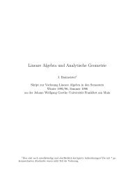
In a typical experiment in particle physics we prepare beams of particles with definitemomentum, polarization, etc. At the same time we measure momenta andpolarizations of the nal states. For this reason it is convenient to work in a momentumrepresentation. The result for a generic matrix element oftheS matrix canbe expressed in the following formhfjSjii =(2) 4 4 ( X inp in ; X outp out )Yext: bosonsr12EVYext: fermionsr mVE M (1.239)Here f 6= i, and we are using the box normalization. The Feynman amplitude M(often one denes a matrix T wich diers from M by a factor i) can be obtained bydrawing at a given perturbative order all the connected and topologically inequivalentFeynman's diagrams. The diagrams are obtained by combining together thegraphics elements given in Figures 1.5.1 and 1.5.2. The amplitude M is given by thesum of the amplitudes associated to these diagrams, after extraction of the factor(2) 4 4 ( P p) in (1.239)..Fermion linePhoton lineScalar lineFig. 1.5.1 - Graphical representation for both internal and external particle lines..QED vertexScalar QED seagullFig. 1.5.2 - Graphical representation for the vertices in scalar and spinor QED.31

At each diagram we associate an amplitude obtained by multiplying together thefollowing factors. for each ingoing and/or outgoing external photon line a factor (or its complexconjugate for outgoing photons if we consider complex polarizations asthe circular one) for each ingoing and/or outgoing external fermionic line a factor u(p) and/oru(p) for each ingoing and/or outgoing external antifermionic line a factor v(p)and/or v(p) for each internal scalar line a factor i F (p) (propagator) for each internal photon line a factor ig D(p) (propagator) for each internal fermion line a factor iS F (p) (propagator) for each vertex in scalar QED a factor ;ie(p + p 0 )(2) 4 4 ( P in p i ; P out p f),where p and p 0 are the momenta of the scalar particle (taking p ingoing and p 0outgoing) For each seagull term in scalar QED a factor 2ie 2 g (2) 4 4 ( P in p i ; P out p f) for each vertex in spinor QED a factor ;ie (2) 4 4 ( P ingoing p i ; P outgoing p f) Integrate over all the internal momenta with measure d 4 p=(2) 4 . This givesrise automatically to the conservation of the total four-momentum. In a graph containing closed lines (loops), a factor (;1) for each fermionicloop (see Fig. 1.5.3)Fermion loopFig. 1.5.3 - A fermion loop can appear inside any Feynman diagram (attaching therest of the diagram by photonic lines).In the following we will use need also the rules for the interaction with a staticexternal e.m. eld. The correspending graphical element isgiven in Fig. 1.5.4. The32

ule is to treat it as a normal photon, except that one needs to substitute the wavefunction of the photon 1=21 () (q) (1.240)2EVwith the Fourier transform of the external eldA ext (~q )=Zd 3 qe ;i~q ~x A ext (~x ) (1.241)where ~q is the momentum in transfer at the vertex where the external eld line isattached to. Also, since the static external eld breaks translational invariance, weloose the factor (2) 3 ( P in ~p in ; P out ~p out)..Fig. 1.5.4 - Graphical representation for an external electromagnetic eld. Theupper end of the line can be attached to any fermion line.1.5.4 The cross-sectionLet us consider a scattering process with a set of initial particles with four momentap i = (E i ~p i ) which collide and produce a set of nal particles with four momentap f =(E f ~p f ). From the rules of the previous Chapter we know that each externalphoton line contributes with a factor (1=2VE) 1=2 , whereas each external fermionicline contributes with (m=V E) 1=2 . Furthermore the conservation of the total fourmomentum gives a term (2) 4 4 ( P i p i ; P f p f). If we exclude the uninterestingcase f = i we can writeS fi =(2) 4 4Xip i ; X fp f! Yfermioni m 1=2VEYbosoni 1=21M (1.242)2VEwhere M is the Feynman amplitude which can be evaluated by using the rules ofthe previous Section.Let us consider the typical case of a two particle collision giving rise to an Nparticles nal state. Therefore, the probability per unit time of the transition isgiven by w = jS fi j 2 withw = V (2) 4 4 (P f ; P i ) Y i1 Y2VE i33f12VE fYfermioni(2m)jMj 2 (1.243)

where, for reasons of convenience, we have writtenmVE =(2m) 12VE(1.244)w gives the probability per unit time of a transition toward a state with well denedquantum numbers, but we are rather interested to the nal states having momentabetween ~p f and ~p f + d~p f . Since in the volume V the momentum is given by ~p =2~n=L, the number of nal states is given by 3Ld 3 p (1.245)2The cross-section is dened as the probability per unit time divided by the ux ofthe ingoing particles, and has the dimensions of a length to the square[t ;1`2t] =[`2](1.246)In fact the ux is dened as v rel = v rel =V , since in our normalization we have aparticle in the volume V , and v rel is the relative velocity of the ingoing particles.For the bosons this follows from the normalization condition of the functions f ~k (x).For the fermions recall that in the box normalization the wave function isr mEV u(p)e;ipx (1.247)from whichZVd 3 x(x) =ZVd 3 x mVE uy (p)u(p) =1 (1.248)Then the cross-section for getting the nal states with momenta between ~p f e ~p f +d~p fis given byd = w V dN F = w V Y Vd 3 p f(1.249)v rel v rel (2) 3We obtaind = Vv relYfVd 3 p f(2) V 1 Y 13 (2)4 4 (P f ; P i )4V 2 E 1 E 2 2VE f1= (2) 4 4 (P f ; P i )4E 1 E 2 v relYffermioni(2m) Y ffYfermioni(2m)jMj 2d 3 p f(2) 3 2E fjMj 2 (1.250)Notice that the dependence on the quantization volume V disappears, as it shouldbe, in the nal equation. Furthermore, the total cross-section, which is obtained byintegrating the previous expression over all the nal momenta, is Lorentz invariant.34

In fact, as it follows from the Feynman rules, M is invariant, as the factors d 3 p=2E.Furthermore~v rel = ~v 1 ; ~v 2 = ~p 1E 1; ~p 2E 2(1.251)but in the frame where the particle 2 is at rest (laboratory frame) we have p 2 =(m 2 ~0) and ~v rel = ~v 1 , from whichE 1 E 2 j~v rel j ==E 1 m 2j~p 1 jE 1= m 2 j~p 1 j = m 2qE 2 1 ; m 2 1qm 2 2E 2 1 ; m 2 1m 2 2 =We see that also this factor is Lorentz invariant.q(p 1 p 2 ) 2 ; m 2 1m 2 2 (1.252)35

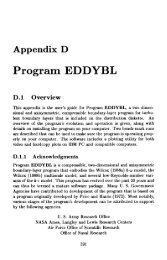
Chapter 2One-loop renormalization2.1 Divergences of the Feynman integralsLet us consider the Coulomb scattering. If we expand the S matrix up to thethird order in the electric charge, and we assume that the external eld is weakenough such totake only the rst order, we can easily see that the relevant Feynmandiagrams are the ones of Fig. 2.1.1. .pkpp−kp’p ’ −pp’p ’ −ppa) b)pkp’k+qc) p ’ −pd)=pp−κpp’p ’ −pp’−kp ’kp ’ −pp’kp ’ −kp ’ −pFig. 2.1.1 - The Feynman diagram for the Coulomb scattering at the third orderin the electric charge and at the rst order in the external eld.36

The Coulomb scattering can be used, in principle, to dene the physical electriccharge of the electron. This is done assuming that the amplitude is linear in e phys ,from which we get an expansion of the typee phys = e + a 2 e 3 + = e(1 + a 2 e 2 + ) (2.1)in terms of the parameter e which appears in the original lagrangian. The rstproblem we encounter is that we would like tohave the results of our calculation interms of measured quantities as e phys . This could be done by inverting the previousexpansion, but, and here comes the second problem, the coecient of the expansionare divergent quantities. To show this, consider, for instance the self-energycontribution to one of the external photons (as the one in Fig. 2.1.1a). We havewhereorM a = u(p 0 )(;ie )A extie 2 (p) =Z= ;e 2 ZZ(p) =id 4 k(2) 4(~p 0 i; ~p)^p ; m + i(;ie ) ;igk 2 + id 4 k(2) 4d 4 k(2) 4 1k 2 + iie 2 (p) u(p) (2.2)i^p ; ^k ; m + i (;ie )1^p ; ^k ; m + i (2.3)^p ; ^k + m 1(p ; k) 2 ; m 2 + i k 2 + i(2.4)For large momentum, k, the integrand behaves as 1=k 3 and the integral divergeslinearly. Analogously one can check that all the other third order contributionsdiverge. Let us write explicitly the amplitudes for the other diagramswhereM b = u(p 0 )ie 2 (p 0 i)^p 0 ; m + i (;ie )A ext (~p 0 ; ~p)u(p) (2.5)M c = u(p 0 )(;ie ) ;ig q 2 + i ie2 (q)A ext (~p 0 ; ~p)u(p) q = p 0 ; p (2.6)ie 2 (q) =(;1)Zd 4 k(2) 4Tr ii^k +^q ; m + i (;ie )^k ; m + i (;ie )(2.7)(the minus sign originates from the fermion loop) and thereforeZ d 4 k(q) =i(2) Tr 114 ^k +^q ; m ^k ; m + i (2.8)The last contribution isM d = u(p 0 )(;ie)e 2 (p 0 p)u(p)A ext (~p 0 ; ~p) (2.9)37

whereore 2 (p 0 p)=ZZ (p 0 p)=;id 4 k(2) 4 (;ie )i^p 0 ; ^k ; m + i d 4 k11(2) 4 ^p 0 ; ^k ; m + i ^p ; ^k ; m + i i^p ; ^k ; m + i (;ie ) ;ig k 2 + i(2.10)1k 2 + i(2.11)The problem of the divergences is a serious one and in order to give some sense tothe theory we have to dene a way to dene our integrals. This is what is called theregularization procedure of the Feynman integrals. That is we give a prescription inorder to make the integrals nite. This can be done in various ways, as introducingan ultraviolet cut-o, or, as we shall see later by the more convenient means ofdimensional regularization. However, we want that the theory does not depend onthe way in which we dene the integrals, otherwise we would have to look for somephysical meaning of the regularization procedure we choose. This bring us to theother problem, the inversion of eq. (2.1). Since now the coecients are nite we canindeed perform the inversion and obtaining e as a function of e phys and obtain allthe observables in terms of the physical electric charge (that is the one measured inthe Coulomb scattering). By doing so, a priori we will introduce in the observablesa dependence on the renormalization procedure. We will say that the theory isrenormalizable when this dependence cancels out. Thinking to the regularization interms of a cut-o this means that considering the observable quantities in terms ofe phys , and removing the cut-o (that is by taking the limit for the cut-o going tothe innity), the result should be nite. Of course, this cancellation is not obviousat all, and in fact in most of the theories this does not happen. However there isa restrict class of renormalizable theories, as for instance QED. We will not discussthe renormalization at all order and neither we will prove which criteria a theoryshould satisfy in order to be renormalizable. We will give these criteria withouta proof but we will try only to justify them On a physical basis. As far QED isconcerned we will study in detail the renormalization at one-loop.2.2 Higher order correctionsIn this section we will illustrate, in a simplied context, the previous considerations.Consider again the Coulomb scattering. At the lowest order the Feynman amplitudein presence of an external static electromagnetic eld is simply given by the followingexpression (see Fig. 2.1.1), (f 6= i)S fi =(2)(E f ; E i ) mVE M(1) (2.12)whereM (1) = u(p 0 )(;ie )u(p)A ext (~p 0 ; ~p ) (2.13)38

andZA ext (~q) =d 3 x A ext (~x)e ;i~q ~x (2.14)is the Fourier transform of the static e.m. eld. In the case of a point-like source,of charge Ze we haveA ext (~x) =(; Ze4j~xj ~0) (2.15)For the following it is more convenient to re-express the previous amplitude in termsof the external current generating the external e.m. eld. Since we havewe can invert this equation in momentum space, by gettingfrom whichwithA = j (2.16)A (q) =; g q 2 + i j (q) (2.17)M (1) = u(p 0 )(;ie )u(p) ;igq 2 + i (;ijext (~p 0 ; ~p)) (2.18)j ext (~x) =(Ze 3 (~x)~0) (2.19)From these expressions one can get easily the dierential cross-section d=d. Thisquantity could be measured and then we could compare the result with the theoreticalresult obtained from the previous expression. In this way we get a measure ofthe electric charge. However the result is tied to a theoretical equation evaluated atthe lowest order in e. In order to get a better determination one has to evaluate thehigher order corrections, and again extract the value of e from the data. The lowestorder result is at the order e 2 in the electric charge. the next-to-leading contributionsar at the order e 4 . For instance, the diagram in Fig. 2.1.1c gives one of thesecontribution. This is usually referred to as the vacuum polarization contributionand in this Section we will consider only this correction, just to exemplify how therenormalization procedure works. This contribution is given in eqs. (2.6) and (2.7).The total result isM (1) + M c = u(p 0 )(;ie )u(p) ;igq 2 + i + ;igq 2 + i (ie2 ) ;ig(;ijq 2 xt (~q))+ i(2.20)The sum gives a result very similar the to one obtained from M (1) alone, but withthe photon propagator modied in the following way;ig q 2! ;igq 2+ ;ig(ie 2 q 2 (q 2 )) ;igq 2= ;igq 2+ ;ie2 q 4 (2.21)39

As discussed in the previous Section is a divergent quantity. In fact, at highvalues of the momentum it behaves asZd4 pp 2 (2.22)and therefore it diverges in a quadratic way. This follows by evaluating the integralby cutting the upper limit by a cut-o . As we shall see later on, the real divergenceis weaker due to the gauge invariance. We will see that the correct behaviour is givenbyZd4 pp 4 (2.23)The corresponding divergence is only logarithmic, but in any case the integral isdivergent. By evaluating it with a cut-o we get (q 2 )=;g q 2 I(q 2 )+ (2.24)The terms omitted are proportional to q q , and since the photon is always attachedto a conserved current, they do not contribute to the nal result. The functions I(q 2 )can be evaluated by various tricks (we will evaluate it explicitly in the following)and the result isZI(q 2 )= 1 2log122 m ; 1 12 2 2 0dz z(1 ; z)log1 ; q2 z(1 ; z)m 2For small values of q 2 (;q 2

in the limit q ! 0 the result looks exactly as at the lowest order, except that weneed to introduce a renormalized charge e R given by 1=2e R = e1 ; e2 2log (2.29)122 m 2In term of e R and taking into account that we are working at the order e 4 we canwrite ;iM (1) + M c = u f (ie R 0 )u i 1 ; e2 R q 2(;iZeq 2 60 2 m 2 R ) (2.30)Now we compare this result with the experiment where we measure d=d in thelimit q ! 0. We can extract again from the data the value of the electric charge, butthis time we will measure e R . Notice that in this expression there are no more divergentquantities,since they have been eliminated by the denition of the renormalizedcharge. It must be stressed that the quantity that is xed by the experiments isnot the "parameter" e appearing in the original lagrangian, but rather e R . Thismeans that the quantity e is not really dened unless we specify how to relate itto measured quantities. This relation is usually referred to as the renormalizationcondition.As we have noticed the nal expression we got does not contain anyexplicit divergent quantity. Furthermore, also e R ,which is obtained from the experimentaldata, is a nite quantity. It follows that the parameter e, must diverge for !1. In other words, the divergence which wehave obtained in the amplitude, iscompensated by the divergence implicit in e. Therefore the procedure outlined herehas meaning only if we start with an innite charge. Said that, the renormalizationprocedure is a way of reorganizing the terms of the perturbative expansion in sucha way that the parameter controlling it is the renormalized charge e R . If this ispossible, the various terms in the expansion turn out to be nite and the theory issaid to be renormalizable. As already stressed this is not automatically satised.In fact renormalizability is not a generic feature of the relativistic quantum eldtheories. Rather the class of renormalizable theories (that is the theories for whichthe previous procedure is meaningful) is quite restricted.We have seen that the measured electric charge is dierent from the quantityappearing in the expression of the vertex. It will be convenient in the following to callthis quantity e B (tha bare charge). On the contrary, the renormalized charge will becalled e, rather than e R as done previously. For the moment being we have includedonly the vacuum polarization corrections, however if we restrict our problem to thecharge renormalization, the divergent part coming from the self-energy and vertexcorrections cancel out (see later). Let us consider now a process like e ; ; ! e ; ; .Neglecting other corrections the total amplitude is given by Fig. 2.2.2.We will dene the charge by choosing an arbitrary value of the square of themomentum in transfer q , such that Q 2 = ;q 2 = 2 . In this way the renormalizedcharge depends on the scale . In the previous example we were using q ! 0. Thegraphs in Fig. 2.2.2 sum up to give (omitting the contribution of the fermionic41

.e Bq + + +e Be −e Beee − e − BBµ−e Be Be Be Be Be Bµ−e Bµ−Fig. 2.2.2 - The vacuum polarization contributions to the e ; ; ! e ; ; scattering.lines,)h ;ige 2 Bq 2+ ;ig(ie 2qB 2 ) ;igq 2+ ;igq 2By considering only the g contribution to ,we geti(ie 2 B ) ;ig(ie 2qB 2 ) ;ig+q 2 Q2 = 2(2.31);ige 2 B 1 ; e2q 2 B I(q 2 )+e 4 BI 2 (q 2 )+ Q2 = 2 (2.32)This expression looks as the lowest order contribution to the propagator be deningthe renormalized electric charge ase 2 = e 2 B[1 ; e 2 BI( 2 )+e 4 BI 2 ( 2 )+] (2.33)Since the fermionic contribution is the same for all the diagrams, by calling it F (Q 2 ),we get the amplitude in the formM(e B )=e 2 BF (Q 2 )[1 ; e 2 BI(Q 2 )+e 4 BI 2 (Q 2 ) ] (2.34)where e 2 BF (Q 2 ) is the amplitude at the lowest order in e 2 B. As we know I(Q 2 ) is adivergent quantity and therefore the amplitude is not dened. However, followingthe discussion of the previous Section we can try to re-express everything in termsof the renormalized charge (2.33). We can easily invert by series the eq. (2.33)obtaining at the order e 4 e 2 B = e 2 [1 + e 2 I( 2 )+] (2.35)42

By substituting this expression in M(e 0 ) we getM(e B ) = e 2 [1 + e 2 I( 2 )+]F (Q 2 )[1 ; e 2 I(Q 2 )+]== e 2 F (Q 2 )[1 ; e 2 (I(Q 2 ) ; I( 2 )) + ] M R (e) (2.36)From the expression (2.25) for I(Q 2 ) we getZI(Q 2 )= 1 2log122 m ; 1 12 2 2 0dz z(1 ; z)log1+ Q2 z(1 ; z)m 2(2.37)Since the divergent part is momentum independent it cancels out in the expressionfor M R (e). Furthermore, the renormalized charge e will be measured through thecross-section, and therefore, by denition, it will be nite. Therefore, the chargerenormalization makes the amplitude nite. Evaluating I(Q 2 ) ; I( 2 )perlarge Q 2(and 2 )we gete 2 (I(Q 2 ) ; I( 2 )) = ; 2 and in this limit! ; 2 Z 10Z 10dz z(1 ; z)logdz z(1 ; z)log Q2 2 m2 + Q 2 z(1 ; z)!m 2 + 2 z(1 ; z)= ; 3M R (e) =e 2 F (Q 2 )1 ; Q2log3 + 2logQ2 2 (2.38)(2.39)At rst sight M R (e) depends on , but actually this is not the case. In fact, e isdened through the eq. (2.33) and therefore it depends also on . What is goingon is that the implicit dependecnce of e on cancels out the explicit dependenceof M R (e). This follows from M R (e) =M(e B ) and on the observation that M(e B )does not depend on . This can be formalized in a way that amounts to introducethe concept of renormalization group that we will discuss in much more detail lateron. In fact, let us be more explicit by writingM(e B )=M R (e()) (2.40)By dierentiating this expression with respect to we getdM(e B )d= @M R@+ @M R@e@e@=0 (2.41)This equation say formally that the amplitude expressed as a function of the renormalizedcharge is indeed independent on . This equation is the prototype of therenormalization group equations, and tells us how we have to change the coupling,when we change the denition scale .Going back to the original expression for M(e 0 ), we see that this is given bythe tree amplitude e 2 BF (Q 2 ) times a geometric series arising from the iteration of43

the vacuum polarization diagram. Therefore, it comes natural to dene a couplingrunning with the momentum of the photon.e 2 (Q 2 )=e 2 B[1 ; e 2 BI(Q 2 )+e 4 BI 2 (Q 2 )+]=e 2 B1+e 2 B I(Q2 )(2.42)Also this expression is cooked up in terms of the divergent quantities e B and I(Q 2 ),but again e 2 (Q 2 ) is nite. This can be shown explicitly by evaluating the renormalizedcharge, e( 2 ), in terms of the bare onee 2 ( 2 )=e 2 B1+e 2 B I(2 )(2.43)We can put the last two equations in the form1e 2 (Q 2 ) = 1e 2 B+ I(Q 2 )1e 2 ( 2 ) = 1e 2 B+ I( 2 ) (2.44)and subtracting them1e 2 (Q 2 ) ; 1e 2 ( 2 ) = I(Q2 ) ; I( 2 ) (2.45)we gete 2 (Q 2 )=By using this result we can write M R (e) ase 2 ( 2 )1+e 2 ( 2 )[I(Q 2 ) ; I( 2 )](2.46)M R (e) =e 2 (Q 2 )F (Q 2 ) (2.47)It follows that the true expansion parameter in the perturbative series is the runningcoupling e(Q 2 ). By using eq. (2.38) we obtain(Q 2 )=( 2 )1 ; (2 )3(2.48)Q2log 2We see that (Q 2 ) increases with Q 2 , therefore the perturbative approach loosesvalidity for those values Q 2 of such that (Q 2 ) 1, that is whenor1 ; (2 )3Q 2 2= e 3Q2log = 2 (2 ) (2.49) 1( 2 ) ; 1 (2.50)44

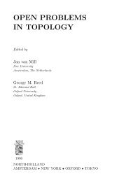
For ( 2 ) 1=137 we getActually (Q 2 ) is divergent forQ 2 2 e1281 10 556 (2.51)Q 2 2= e 3( 2) e 1291 10 560 (2.52)This value of Q 2 is referred to as the Landau pole. Therefore in the case of QED theperturbative approach maintains its validity upto gigantic values of the momenta.This discussion shows clearly that the behaviour of the running coupling constantis determined by I(Q 2 ), that is from the vaccum polarization contribution. In particular,(Q 2 ) increases with Q 2 since in the expression e 2 ( 2 )(I(Q 2 ) ; I( 2 )) thecoecient of the logarithm is negative (equal to ;( 2 )=(3)). We will see that inthe so called non-abelian gauge theories the running is opposite, that is the theorybecomes more and more perturbative, by increasing the energy.2.3 The analysis by countertermsThe previous way of dening a renormalizable theory amounts to say that the originalparameters in the lagrangian, as e, should be innite and that their divergencesshould compensate the divergences of the Feynman diagrams. Then one can try toseparate the innite from the nite part of the parameters (this separation is ambiguous,see later). The innite contributions are called counterterms, and by denitionthey have the same operator structure of the original terms in the lagrangian. Onthe other hand, the procedure of regularization can be performed by adding to theoriginal lagrangian counterterms cooked in such a way that their contribution killsthe divergent part of the Feynman integrals. This means that the coecients ofthese counterterms have to be innite. However they can also be regularized in thesame way as the other integrals. We see that the theory will be renormalizable ifthe counterterms we add to make the theory nite have the same structure of theoriginal terms in the lagrangian, in fact, if this is the case, they can be absorbedin the original parameters, which however are arbitrary, because they have to bexed by the experiments (renormalization conditions). We will show now that atone-loop the divergent contributions come only from the three diagrams discussedbefore. In fact, let us dene D as the supercial degree of divergence of a one-loopdiagram the dierence between 4 (the number of integration over the mimentum)and the number of powers of momentum coming from the propagators (we assumehere that no powers of momenta are coming from the vertices, which is not true inscalar QED). We getD =4; I F ; 2I B (2.53)45

where I F and I B are the number of internal fermionic and bosonic lines. Goingthrough the loop one has to have a number of vertices, V equal to the number ofinternal linesV = I F + I B (2.54)Also, if at each vertex there are N i lines of the particle of type i, then we haveN i V =2I i + E i (2.55)from which2V =2I F + E F V =2I B + E B (2.56)From these equations we can get V , I F and I B in terms of E F and E BI F = 1 2 E F + E B I B = 1 2 E F V = E F + E B (2.57)from whichD =4; 3 2 E F ; E B (2.58)It follows that the only one-loop supercially divergent diagrams in spinor QED arethe ones in Fig. 2.3.1. In fact, all the diagrams with an odd number of externalphotons vanish. This is trivial at one-loop, since the trace of an odd number of matrices is zero. In general (Furry's theorem) it follows from the conservation ofcharge conjugation, since the photon is an eigenstate of C with eigenvalue equal to-1.Furthermore, the eective degree of divergence can be less than the supercialdegree. In fact, gauge invariance often lowers the divergence. For instance thediagram of Fig. 2.3.1 with four external photons (light-light scattering) has D =0(logarithmic divergence), but gauge invariance makes it nite. Also the vacuumpolarization diagram has an eective degree of divergence equal to 2. Therefore,there are only three divergent one-loop diagrams and all the divergences can bebrought back to the three functions (p), (q) e (p 0 p). This does not meanthat an arbitrary diagram is not divergence, but it can be made nite if the previousfunctions are such. In such a case one has only to show that eliminating these threedivergences (primitive divergences) the theory is automatically nite. In particularwe will show that the divergent part of (p) can be absorbed into the denitionof the mass of the electron and a redenition of the electron eld (wave functionrenormalization). The divergence in , the photon self-energy, can be absorbedin the wave function renormalization of the photon (the mass of the photon is notrenormalized due to the gauge invariance). And nally the divergence of (p 0 p)goes into the denition of the parameter e. To realize this program we divide upthe lagrangian density intwo parts, one written in terms of the physical parameters,the other will contain the counterterms. We will call also the original parametersand elds of the theory the bare parameters and the bare elds and we will use anindex B in order to distinguish them from the physical quantities. Therefore the46

.EEF BD0 2 20 4 02 0 12 1 0Fig. 2.3.1 - The supercially divergent one-loop diagrams in spinor QEDtwo pieces of the lagrangian should look like as follows: the piece in terms of thephysical parametersL pL p = (i^@ ; m) ; e A ; 1 4 F F ; 1 2 (@ A ) 2 (2.59)and the counter terms piece L c:t:L c:t: = iB ^@ ; A ; C 4 F ; E 2 (@ A ) 2 ; eD ^A (2.60)and we have to require that la sum of these two contributions should coincide withthe original lagrangian written in terms of the bare quantities. Adding together L pand L c:t: we getL =(1+B)i ^@ ; (m + A) ; e(1 + D) A ; 1+C F F + gauge ; xing4(2.61)where, for sake of simplicity, we have omitted the gauge xing term. Dening therenormalization constant of the eldswe write the bare elds asZ 1 =(1+D) Z 2 =(1+B) Z 3 =(1+C) (2.62)B = Z 1=22 A B = Z1=2 3 A (2.63)47

we obtainL = i ^@ B B ; m + A B B ; eZ 1Z 2 Z 2 Z 1=2 B B A B; 1 4 F BF B+ gauge ; xing3(2.64)and puttingwe getm B = m + AZ 2 e B = eZ 1Z 2 Z 1=23L = i B ^@ B ; m B B B ; e B B B A B; 1 4 F BF B(2.65)+ gauge ; xing (2.66)So we have succeeded in the wanted separation. Notice that the division of the parametersin physical and counter term part is well dened, because the nite pieceis xed to be an observable quantity. This requirement gives the renormalizationconditions. The counter terms A, B, ... are determined recursively at each perturbativeorder in such a way to eliminate the divergent parts and to respect therenormalization conditions. We will see later how thisworks in practice at one-looplevel. Another observation is that Z 1 and Z 2 have to do with the self-energy of theelectron, and as such they depend on the electron mass. Therefore if we considerthe theory for a dierent particle, as the muon, which has the same interactions asthe electron and diers only for the value of the mass (m 200m e ), one wouldget a dierent bare electric charge for the two particles. Or, phrased in a dierentway, one would have to tune the bare electric charge at dierent values in order toget the same physical charge. This looks very unnatural, but the gauge invarianceof the theory implies that at all the perturbative orders Z 1 = Z 2 . As a consequencee B = e=Z 1=23 , and since Z 3 comes from the photon self-energy, the relation betweenthe bare and the physical electric charge is universal (that is it does not depend onthe kind of charged particle under consideration).Summarizing, one starts dividing the bare lagrangian in two pieces. Then weregularize the theory giving some prescription to get nite Feynman integrals. Thepart containing the counter terms is determined, order by order, by requiring thatthe divergences of the Feynman integrals, which come about when removing theregularization, are cancelled out by the counter term contributions. Since the separationof an innite quantity into an innite plus a nite term is not well dened, weuse the renormalization conditions, to x the nite part. After evaluating a physicalquantity we remove the regularization. Notice that although the counter terms aredivergent quantity when we remove the cut o, we will order them according to thepower of the coupling in which we are doing the perturbative calculation. That is wehave a double limit, one in the coupling and the other in some parameter (regulator)which denes the regularization. The order of the limit is rst to work at some orderin the coupling, at xed regulator, and then remove the regularization.Before going into the calculations for QED we want to illustrate some generalresults about the renormalization. If one considers only theory involving scalar,48

fermion and massless spin 1 (as the photon) elds, it is not dicult to constructan algorithm which allows to evaluate the ultraviolet (that is for large momenta)divergence of any Feynman diagram. In the case of the electron self-energy (seeFigs. 2.1.1a and 2.1.1b) one has an integration over the four momentum p and abehaviour of the integrand, coming from the propagators, as 1=p 3 , giving a lineardivergence (it turns out that the divergence is only logarithmic). From this countingone can see that only the lagrangian densities containing monomials in the eldswith mass dimension smaller or equal to the number of space-time dimensions haveanitenumber of divergent diagrams. It turns out also that these are renormalizabletheories ( a part some small technicalities). The mass dimensions of the elds can beeasily evaluated from the observation that the action is dimensionless in our units(h/ = 1). Therefore, in n space-time dimensions, the lagrangian density, dened asZd n x L (2.67)has a mass dimension n. Looking at the kinetic terms of the bosonic elds (twoderivatives) and of the fermionic elds (one derivative), we see thatdim[] = dim[A ]= n 2; 1 dim[ ] =n; 12(2.68)In particular, in 4 dimensions the bosonic elds have dimension 1 and the fermionic3=2. Then, we see that QED is renormalizable, since all the terms in the lagrangiandensity have dimensions smaller or equal to 4dim[ ]=3 dim[ A ]=4 dim[(@ A ) 2 ]=4 (2.69)The condition on the dimensions of the operators appearing in the lagrangian canbe translated into a condition over the coupling constants. In fact each monomialO i will appear multiplied by a coupling g iL = X ig i O i (2.70)thereforeThe renormalizability requiresfrom whichdim[g i ]=4; dim[O i ] (2.71)dim[O i ] 4 (2.72)dim[g i ] 0 (2.73)that is the couplings must have positive dimension in mass are to be dimensionless.In QED the only couplings are the mass of the electron and the electric charge49

which is dimensionless. As a further example consider a single scalar eld. Themost general renormalizable lagrangian density is characterized by two parametersL = 1 2 @ @ ; 1 2 m2 2 ; 3 ; 4 (2.74)Here has dimension 1 and is dimensionless. We see that the linear -models arerenormalizable theories.Giving these facts let us try to understand what makes renormalizable and nonrenormalizable theories dierent. In the renormalizable case, if we have writtenthe most general lagrangian, the only divergent diagrams which appear are theones corresponding to the processes described by the operators appearing in thelagrangian. Therefore adding to L the counter termL c:t: = X ig i O i (2.75)we can choose the g i in such away to cancel, order by order, the divergences. Thetheory depends on a nite number of arbitrary parameters equal to the number ofparameters g i . Therefore the theory is a predictive one. In the non renormalizablecase, the number of divergent diagrams increase with the perturbative order. Ateach order we have to introduce new counter terms having an operator structuredierent from the original one. At the end the theory will depend on an innitenumber of arbitrary parameters. As an example consider a fermionic theory with aninteraction of the type ( ) 2 . Since this term has dimension 6, the relative couplinghas dimension -2L int = ;g 2 ( ) 2 (2.76)At one loop the theory gives rise to the divergent diagrams of Fig. 2.3.2. Thedivergence of the rst diagram can be absorbed into a counter term of the originaltype;g 2 ( ) 2 (2.77)The other two need counter termsofthetypeg 3 ( ) 3 + g 4 ( ) 4 (2.78)These counter terms originate new one-loop divergent diagrams, as for instance theones in Fig. 2.3.3. The rst diagram modies the already introduced counter term( ) 4 ,butthe second one needs anewcounter termg 5 ( ) 5 (2.79)This process never ends.The renormalization requirement restricts in a fantastic way the possible eldtheories. However one could think that this requirement is too technical and onecould imagine other ways of giving a meaning to lagrangians which do not satisfy this50

.a) b)c)Fig. 2.3.2 - Divergent diagrams coming from the interaction ( ) 2 .condition. But suppose we try to give a meaning to a non renormalizable lagrangian,simply requiring that it gives rise to a consistent theory at any energy. We will showthat this does not happen. Consider again a theory with a four-fermion interaction.Since dim g 2 = ;2, if we consider the scattering + ! + in the high energylimit (where we can neglect all the masses), on dimensional ground we get that thetotal cross-section behaves like g 2 2E 2 (2.80)Analogously, inany non renormalizable theory, being there couplings with negativedimensions, the cross-section will increase with the energy. But the cross-section hasto do with the S matrix which is unitary. Since a unitary matrix has eigenvalues of.a) b)Fig. 2.3.3 - Divergent diagrams coming from the interactions ( ) 2 and ( ) 4 .51

modulus 1, it follows that its matrix elements must be bounded. Translating thisargument in the cross-section one gets the boundwhere c is some constant. For the previous example we get c2E 2 (2.81)g 2 E 2 c (2.82)This implies a violation of the S matrix unitarity at energies such thatE r cg 2(2.83)It follows that we can give a meaning also to non renormalizable theories, but onlyfor a limited range of values of the energy. This range is xed by the value of thenon renormalizable coupling. It is not diculty to realize that non renormalizabilityand bad behaviour of the amplitudes at high energies are strictly connected.2.4 Dimensional regularization of the FeynmanintegralsAs we have discussed in the previous Section we need a procedure to give sense atthe otherwise divergent Feynman diagrams. The simplest R of these procedures is just1 Rto introduce a cut-o and dene our integrals as !lim0 !1 ). Of course,0in the spirit of renormalization we have rst to perform the perturbative expansionand then take the limit over the cut-o. Although this procedure is very simple itresults to be inadequate in situations like gauge theories. In fact one can show thatthe cut-o regularization breaks the translational invariance and creates problemsin gauge theories. One kind of regularization which nowadays is very much used isthe dimensional regularization. This consists in considering the integration in anarbitrary number of space-time dimensions and taking the limit of four dimensionsat the end. This way of regularizing is very convenient because it respects all thesymmetries. In fact, except for very few cases the symmetries do not depend on thenumber of space-time dimensions. Let us what is dimensional regularization about.We want to evaluate integrals of the typeI 4 (k) =Zd 4 pF(p k) (2.84)with F (p k) p ;2 or p ;4 . The idea is that integrating on a lower number ofdimensions the integral improves the convergence properties in the ultraviolet. For52

instance, if F (p k) p ;4 , the integral is convergent in 2 and in 3 dimensions.Therefore, we would like tointroduce aquantityI(! k) =Zd 2! p F (p k) (2.85)to be regarded as a function of the complex variable !. Then, if we can denea complex function I 0 (! k) on the entire complex plane, with denite singularity,and as such that it coincides with I on some common domain, then by analyticcontinuation I and I 0 dene the same analytic function. A simple example of thisprocedure is given by the Euler's ;. This complex function is dened for Re z > 0by the integral representation;(z) =If Re z 0, the integral diverges asZ 10dt e ;t t z;1 (2.86)dtt 1+jRe zj (2.87)in the limit t ! 0.However it is easy to get a representation valid also for Re z 0.Let us divide the integration region in two parts dened by a parameter ;(z) =Z 0dt e ;t t z;1 +Z 1dt e ;t t z;1 (2.88)Expanding the exponential in the rst integral and integrating term by term we get;(z) ==1X1Xn=0n=0(;1) nn!(;1) nn!Z 0dt t n+z;1 +Z n+z 1n + z +Z 1dt e ;t t z;1dt e ;t t z;1 (2.89)The second integral converges for any z since >0. This expression coincides withthe representation for the ; function for Re z > 0, but it is dened also for Re z < 0where it has simple poles located at z = ;n. Therefore it is a meaningful expressionon all the complex plane z. Notice that in order to isolate the divergences we needto introduce an arbitrary parameter . However the result does not depend on theparticular value of this parameter. This the Weierstrass representation of the Euler;(z). From this example we see that we need the following three steps Find a domain where I(! k)isconvergent. Typically this will be for Re !

2.5 Integration in arbitrary dimensionsLet us consider the integralI N =Zd N pF (p 2 ) (2.90)with N an integer number and p a vector in an Euclidean N-dimensional space.Since the integrand is invariant under rotations of the N-dimensional vector p, wecan perform the angular integration by means ofd N p = d N p N;1 dp (2.91)where d N is the solid angle element inN-dimensions. Therefore R d N = S N , withS N the surface of the unit sphere in N-dimensions. ThenZ 1I N = S N p N;1 F (p 2 )dp (2.92)0The value of the sphere surface can be evaluated by the following trick. ConsiderI =Z +1;1e ;x2 dx = p (2.93)By taking N of these factors we getI N =Zdx 1 dx N e ;(x2 1 + + x 2 N) = N=2(2.94)The same integral can be evaluated in polar coordinatesZ 1 N=2 = S N N;1 e ;2 d (2.95)0By putting x = 2 we have N=2 = 1 2 S NZ 10 x N=2;1 e ;x dx = 1 N2 S N;2(2.96)where we have used the representation of the Euler ; function given in the previousSection. ThereforeS N = 2N=2; (2.97)N;2andI N = N=2; Z 1x N=2;1 F (x)dx (2.98)N;2 0with x = p 2 .54

The integrals we will be interested in are of the typeI (M)N=Zd N p(p 2 ; a 2 + i) A (2.99)with p a vector in a Ndimensional Minkowski space. We can perform an anticlockwiserotation of 90 0 (Wick's rotation) in the complex plane of p 0 without hittingany singularity. P Then wedoachange of variables p 0 ! ip 0 ,andwe use the denitionp 2 !;p 2 N=i=1 p2 i , obtainingI (M)N= iZd N p(;p 2 ; a 2 ) A = i(;1)A I N (2.100)where I N is an integral of the kind discussed at the beginning of this Section withF (x) given byF (x) =(x + a 2 ) ;A (2.101)It followsI N = N=2; N;2By putting x = a 2 y we getI N =(a 2 )N=2;A N=2; ; N2 Z 10 Z 10x N=2;1dx (2.102)(x + a 2 )Ay N=2;1 (1 + y) ;A dx (2.103)and recalling the integral representation for the Euler B(x y) function (valid forRex y > 0)ZB(x y) = ;(x);(y) 1;(x + y) = t x;1 (1 + t) ;(x+y) dt0(2.104)it followsN=2 ;(A ; N=2) 1I N = ;(A) (a 2 ) A;N=2 (2.105)We have obtained this representation for N=2 > 0 and Re(A ; N=2) > 0. But weknow how to extend the Euler gamma-function to the entire complex plane, andtherefore we can extend this formula to complex dimensions N =2!This shows that I 2! has simple poles located at!;(A ; !) 1I 2! = (2.106);(A) (a 2 ) A;!! = A A +1 (2.107)Therefore our integral will be perfectly dened at all ! such that ! 6= A A +1 .At the end we will have to consider the limit ! ! 2. The original integral inMinkowski space is thenZd 2! p(p 2 ; a 2 ) = A i! A ;(A ; !) 1(;1) (2.108);(A) (a 2 ) A;!55

For the following it will be useful to derive another formula.previous equation p = p 0 + k and b 2 = ;a 2 + k 2 , thenZd 2! p 0(p 02 +2p 0 k + k 2 ; a 2 ) A = i! (;1)Let us put in theA;(A ; !) 1(2.109);(A) (a 2 ) A;!from whichZd 2! p(p 2 +2p k + b 2 ) = A i! A ;(A ; !)(;1);(A)1(2.110)(k 2 ; b 2 ) A;!Dierentiating with respect to k we get various useful relations asZd 2! p p(p 2 +2p k + b 2 ) = A i! A ;(A ; !) ;k (;1) (2.111);(A) (k 2 ; b 2 ) A;!andZd 2! p p p(p 2 +2p k + b 2 ) = i ! (;1) AA ;(A)(k 2 ; b 2 ) A;!;(A ; !)k k ; 1 2 g (k 2 ; b 2 );(A ; ! ; 1)(2.112)Since at the end of our calculation we will have to take the limit ! ! 2, it will beuseful to recall the expansion of the Gamma function around its poles;() = 1 ; + O() (2.113)whereis the Euler-Mascheroni constant, and for (n 1):;(;n + ) = (;1)nn! =0:5772::: (2.114) 1 + (n +1)+O() (2.115)where(n +1)=1+ 1 2 + + 1 n ; (2.116)2.6 One loop regularization of QEDIn this Section we will regularize, by using dimensional regularization, the relevantdivergent quantities in QED, that is (p), (q) e (p p 0 ). Furthermore, in orderto dene the counter terms we will determine the expressions which become divergentin the limit of ! ! 2. It will be also convenient to introduce a parameter suchthat these quantities have the same dimensions in the space with d =2! as in d =4.56

The algebra of the Dirac matrices is also easily extended to arbitrary dimensions d.For instance, starting from[ ] +=2g (2.117)we getand = d (2.118) =(2; d) (2.119)Other relations can be obtained by starting from the algebraic properties of the-matrices. Let us start with the electron self-energy which we will require to havedimension 1 as in d =4. From eq. (2.4) we haveZ(p) =i 4;2! d 2! k(2) ^p ; ^k + m 12! (p ; k) 2 ; m 2 + i (2.120)k 2 + iIn order to use the equations of the previous Section it is convenient to combinetogether the denominators of this expression into a single one. This is done by usinga formula due to Feynmanwhich is proven usingand doing the change of variablesZ1 1ab = dz(2.121)[az + b(1 ; z)] 20 1ab = 1 1Zb ; a a ; 1 = 1 bdx(2.122)b b ; a a x 2x = az + b(1 ; z) (2.123)We get(p) =i 4;2! Z 10dzZd 2! k(2) 2! ^p ; ^k + m[(p ; k) 2 z ; m 2 z + k 2 (1 ; z)] 2 (2.124)The denominator can be written in the following way[:::] =p 2 z ; m 2 z + k 2 ; 2p kz (2.125)and the term p k can be eliminated through the following change of variablesk = k 0 + pz. We nd[:::] =(p 2 ; m 2 )z +(k 0 + pz) 2 ; 2p (k 0 + pz)z = k 0 2; m 2 z + p 2 z(1 ; z) (2.126)57

It follows (we put k 0 = k)(p) =i 4;2! Z 10dzZd 2! k(2) 2! The linear term in k has vanishing integral, therefore(p) =i 4;2! Z 1and integrating over k(p) =i 4;2! Z 100dzBy dening =4; 2! we get(p) =; Z 1Contracting the matriceswe obtainDening0Z(p) =; 116 2 ;(=2) Z 1(p) = 116 ;(=2)2Z 10d 2! k(2) 2! 1 ;(2 ; !)dz i!(2)2!;(2)^p(1 ; z) ; ^k + m[k 2 ; m 2 z + p 2 z(1 ; z)] 2 (2.127)^p(1 ; z)+m[k 2 ; m 2 z + p 2 z(1 ; z)] 2 (2.128) 1dz(2) 4; (4;)=2 ;(=2) 0^p(1 ; z)+m[m 2 z ; p 2 z(1 ; z)] 2;! (2.129)^p(1 ; z)+m[m 2 z ; p 2 z(1 ; z)] =2 (2.130)dz(4 2 =2 ( ; 2)^p(1 ; z)+(4; )m) (2.131)[m 2 z ; p 2 z(1 ; z)] =2m2 z ; pdz[2^p(1 ; z) ; 4m ; (^p(1 ; z) ; 2 z(1 ; z)m)]4 2 ;=2(2.132)A =2^p(1 ; z) ; 4m B = ;^p(1 ; z)+m C = m2 z ; p 2 z(1 ; z)4 2 (2.133)and expanding for ! 0(p) ===Z1 116 2 0Z1 116 20dzdz 2A +2B ; A h1 ; 2 log C i 2A ; A log C +2B ; A 11(^p ; 4m) ; [^p ; 2m + (^p ; 4m)]8 2 162 ; 18 2 Z 1=0dz[^p(1 ; z) ; 2m]log m2 z ; p 2 z(1 ; z)4 21(^p ; 4m) + nite terms (2.134)8 2 58

Consider now the vacuum polarization (see eq. (2.8))Z (q) = i 4;2! d 2! k(2) Tr 1 12! ^k +^q ; m Z= i 4;2!^k ; m d 2! k Tr[ (^k + m) (^k +^q + m)](2) 2! (k 2 ; m 2 )((k + q) 2 ; m 2 )Using again the Feynman representation for the denominators (q) =i 4;2! Z 10dzWe write the denominator asZd 2! k(2) 2!(2.135)Tr[ (^k + m) (^k +^q + m)][(k 2 ; m 2 )(1 ; z)+((k + q) 2 ; m 2 )z] 2 (2.136)[:::] =k 2 + q 2 z ; m 2 +2k qz (2.137)through the change of variable k = k 0 ; qz we cancel the mixed term obtaining[:::] =(k 0 ; qz) 2 +2(k 0 ; qz) qz + q 2 z ; m 2 = k 02 + q 2 z(1 ; z) ; m 2 (2.138)and therefore (we put again k 0 = k) (q) =i 4;2! Z 10dzZd 2! k(2) 2! Tr[ (^k ; ^qz + m) (^k +^q(1 ; z)+m)][k 2 + q 2 z(1 ; z) ; m 2 ] 2 (2.139)Since the integral of the odd terms in k is zero, it is enough to evaluate the contributionof the even term to the traceTr[:::] even = Tr[ (^k ; ^qz + m) (^k +^q(1 ; z)] pari + m 2 Tr[ ]= Tr[ ^k^k] ; Tr[^q ^q]z(1 ; z)+m 2 Tr[ ] (2.140)If we dene the as matrices of dimension 2 ! 2 ! we can repeat the standardcalculation by obtaining a factor 2 ! instead of 4. Thereforeand we ndTr[:::] even =2 ! [2k k ; g k 2 ; (2q q ; g q 2 )z(1 ; z)+m 2 g ]=2 ! [2k k ; 2z(1 ; z)(q q ; g q 2 ) ; g (k 2 ; m 2 + q 2 z(1 ; z)](2.141) (q) = i 4;2! 2 ! Z 10dzZd 2! kh(2) 2!2k k [k 2 + q 2 z(1 ; z) ; m 2 ] 2; 2z(1 ; z)(q q ; g q 2 )[k 2 + q 2 z(1 ; z) ; m 2 ] 2 ; g [k 2 + q 2 z(1 ; z) ; m 2 ]From the relations of the previous Section we getZi(2.142)d 2! p2p p [p 2 ; a 2 ] = ;ig ! ;(1 ; !) (2.143)2 (a 2 ) 1;!59

whereasZd 2! 1p[p 2 ; a 2 ]0= ;i!;(1 ; !)(a 2 ) 1;! (2.144)Therefore the rst and the third contribution to the vacuum polarization cancel outand we are left withZ 1Z (q) =;i 4;2! 2 ! (q q ;g q 2 ) dz 2z(1;z)d 2! k1(2) 2! [k 2 + q 2 z(1 ; z) ; m 2 ] 2(2.145)Notice that the original integral was quadratically divergent, but due to the previouscancellation the divergence is only logarithmic. The reason is again gauge invariance.In fact it is possible to show that this implies q (q) =0. Performing themomentum integration we have (q) =;i2 4;2! 2 ! (q q ; g q 2 )Z 10dz z(1 ; z) i!(2) 2! ;(2 ; !)[m 2 ; q 2 z(1 ; z)] 2;!(2.146)By putting again =4; 2! and expanding the previous expression (q) = 2 2 2;=2 (q q ; g q 2 )==Z 1216 2 22;=2 (q q ; g q 2 )20Z 1dz z(1 ; z) 2;=2(2) 4;16 (4 ; 2 log 2)(q q 2 ; g q 2 )Z 1dz z(1 ; z)( 2 h ; ) 1 ; i2 log C0where C is denite in eq. (2.133). Finally (q) = 18 2 (q q ; g q 2 )= 12 (q q 2 ; g q 2 ) 13 ; 6 ; Zor, in abbreviated wayZ0dz z(1 ; z);(=2)dz z(1 ; z)dz z(1 ; z)log;(=2)[m 2 ; q 2 z(1 ; z)] =2m2 ; q 2 z(1 ; z)4 2 ;=2(2.147) 8 ; 4 ; 4 log 2 h1 ; 2 log C im2 ; q 2 z(1 ; z)2 2(2.148) (q) = 16 (q q 2 ; g q 2 ) 1 +niteterms (2.149)We have now to evaluate (p 0 p). From eq. (2.11) we haveZ (p 0 p)=;i 4;2! d 2! k ^p 0 ; ^k + m(2)2!^p ; ^k + m(p 0 ; k) 2 ; m 2 (p ; k) 2 ; m 2 601(2.150)k 2

the general formula to reduce n denominators to a single one isnYi=11a i=(n ; 1)!To show this equation notice thatIntroducing the identitynYi=1Z 1Z1 1=a i 01=and changing variables i = i=nYi=1Z 10Z1 1=a i 0nYi=1Z 10nYi=10nYi=1nYi=1d i n d e ;d i(1 ; P ni=1 i)[ P ni=1 ia i ] n (2.151);d i ed( ;nXi=1d i d( ;nXi=1nXi=1 i a i(2.152) i ) (2.153)nXi=1 i a i(1 ;; i )enXi=1nXi=1 i a i i ) (2.154)The integration over ican be restricted to the interval [0 1] due to the deltafunction, and furthermoreZ 1d n;1 e ; =In our case we getThe denominator is (p 0 p)=;2i 4;2! Z0d 2! k(2) 2! Z 1(n ; 1)! n (2.155)0dxZ 1;x (^p 0 ; ^k + m) (^p ; ^k + m [k 2 (1 ; x ; y)+(p ; k) 2 x ; m 2 x +(p 0 (2.156); k) 2 y ; m 2 y] 3[:::] =k 2 ; m 2 (x + y)+p 2 x + p 02 y ; 2k (px + p 0 y) (2.157)Changing variable, k = k 0 + px + py[:::] = (k 0 + px + p 0 y) 2 ; m 2 (x + y)+p 2 x + p 02 y ; 2(k 0 + px + p 0 y) (px + p 0 y)= k 0 2 ; m 2 (x + y)+p 2 x(1 ; x)+p 02 y(1 ; y) ; 2p p 0 xy (2.158)610dy

Letting again k 0 ! kZ 1 (p 0 p)=;2i 4;2! dx0Z 1;x0Zdyd 2! k(2) 2! (^p 0 (1 ; y) ; ^px ; ^k + m) (^p(1 ; x) ; ^p 0 y ; ^k + m) [k 2 ; m 2 (x + y)+p 2 x(1 ; x)+p 0 2y(1 ; y) ; 2p p 0 xy] 3 (2.159)The odd term in k is zero after integration, the term in k 2 is logarithmically divergent,whereas the remaining part is convergent. Separating the divergent piece, (1) , from the convergent one, (3) ,we get for the rst term (1) (p 0 p) = ;2i 4;2! Z 1Using the relation0 Z 1= ;2i 4;2! dx0 = (1) + (2) (2.160)Z 1;x Zdx dy00d 2! k(2) 2!k k [k 2 ; m 2 (x + y)+p 2 x(1 ; x)+p 0 2y(1 ; y) ; 2p p 0 xy]Z 31;x dy i! (;1) 3; 1 ;(2 ; !);(3) 2 [m 2 (x + y) ; p 2 x(1 ; x) ; p 02 y(1 ; y)+2p p 0 xy] 2;!! 1;(2 ; !)Z= 1 2 4;2! 14we obtain ( =4; 2!)0dxZ 1;x0 [m 2 (x + y) ; p 2 x(1 ; x) ; p 02 y(1 ; y)+2p p 0 xy] 2;! (2.161) (1) (p 0 p)= 1 2 14dy =(2; d) 2 (2.162) 2;=2;(=2)( ; 2) 2 Z 11[m 2 (x + y) ; p 2 x(1 ; x) ; p 0 2y(1 ; y)+2p p 0 xy] =2= 132 2 2 ; [4 ; 4] Z 10dxZ 1;x0 0 m2 (x + y) ; p 2 x(1 ; x) ; p 02 y(1 ; y)+2p p 0 ;=2xydxZ 1;xdy0dy4 2= 18 2 ; 116 2 ( +2) ; 18 2 Z 10dxZ 1;x0dy62

logm2 (x + y) ; p 2 x(1 ; x) ; p 02 y(1 ; y)+2p p 0 xy4 2(2.163)and nally (1) (p 0 p)= 18 2 + nite terms (2.164)In the convergent part we can put directly ! =2 (2) (p 0 p) = ; i8 4 Z 10dxZ 1;x0dy i2 (;1) 3;(3) (^p 0 (1 ; y) ; ^px + m) (^p(1 ; x) ; ^p 0 y + m) m 2 (x + y) ; p 2 x(1 ; x) ; p 02 y(1 ; y)+2p p 0 xyZ= ; 1 1Z 1;xdx dy16 2 0 0 (^p 0 (1 ; y) ; ^px + m) (^p(1 ; x) ; ^p 0 y + m) m 2 (x + y) ; p 2 x(1 ; x) ; p 0 2y(1 ; y)+2p p 0 xy(2.165)2.7 One loop renormalizationWe summarize here the results of the previous Section(p) = 18 2 (^p ; 4m)+f (p) (2.166) 1 (q) =(q q ; g q 2 )6 2 +f (q) (q q ; g q 2 )(q 2 ) (2.167) (p 0 p)= 18 2 + f (p 0 p) (2.168)where the functions with the superscript f represent the nite contributions. Letus start discussing the electron self-energy. As shown in eq. (2.2), the eect of (p)is to correct the electron propagator. In fact we have (see Fig. 2.7.1):.S F (p) =i^p ; m +ii^p ; m ie2 (p) + (2.169)^p ; mFig. 2.7.1 - The loop expansion for the electron propagator.from which, at the same order in the perturbative expansion S F (p) =i;11+ e2 (p)i=^p ; m ^p ; m ^p ; m + e 2 (p)(2.170)63

Therefore the eect of the divergent terms is to modify the coecients of ^p and m: iS ;1F(p) =^p ; m + e2 (p) =^p1+ e2; m1+ e2+nite terms (2.171)8 2 2 2 This allows us to dene the counter terms to be added to the lagrangian expressedin terms of the physical parameters in such away to cancel these divergences(L 1 ) ct = iB ^@ ; A (2.172)(L 1 ) ct modies the Feynman rules adding two particles interacting terms. Thesecan be easily evaluated noticing that the expression of the propagator, taking intoaccount (L 1 ) ct , isi(1 + B)^p ; (m + A)1 ; B ^p ; Ai^p ; m ^p ; mi^p ; m + ii(iB ^p ; iA)^p ; m^p ; m(2.173)where, consistently with our expansion we have taken only the rst order terms inA and B. We can associate to these two terms the diagrams of Fig. 2.7.2, withcontributions ;iA to the mass term, and iB ^p to ^p..-iAiBp/Fig. 2.7.2 - The counter terms for the self-energy (p/ in the gure should be read as^p).The propagator at the second order in the coupling constant is then given by addingthe diagrams of Fig. 2.7.3.At this order we getS F (p) =i^p ; m +i ;ie^p ; 2 (p)+iB ^p ; iiAm^p ; mand the correction to the free propagator is given bye 2 (p)+B ^p ; A = e28 2 + B ^p ;(2.174) e22 2 m + A + nite terms (2.175)We can now x the counter terms by choosingB = ; e28 2 1 + F 2 m(2.176)64

.=Fig. 2.7.3 - The second order contributions at the electron propagator. A = ; me2 1 m2 2 + F m(2.177)with F 2 andF m nite for ! 0. Notice also that these two functions are dimensionlessand arbitrary up to this moment. However they can be determined by therenormalization conditions, that is by xing the arbitrary constants appearing inthe lagrangian. In fact, giveniS ;1F (p) ;(2) (p) =^p ; m + B ^p ; A + e 2 (p) (2.178)we can require that at the physical pole, ^p = m, the propagator coincides with thefree propagatorS F (p) i for ^p = m (2.179)^p ; mFrom here we get two conditions. The rst one is0=; (2) (^p = m) = e28 2 (^p;4m)+e2 f (^p = m); e28 2 1 + F 2from which ^p+ me2 12 2 + F m(2.180)e 2 f (^p = m) ; me28 F 2 2 + me22 F 2 m =0 (2.181)The second condition is@; (2) (p) =1@ ^p ^p=m(2.182)65

which givese 2 @f (p)@ ^p^p=m; e28 2 F 2 =0 (2.183)One should be careful because these particular conditions of renormalization givessome problems related to the zero mass of the photon. In fact one nds some illdenedintegral in the infrared region. However these are harmless divergences,because giving a small to the photon and letting it to zero at the end of the calculationsgives rise to nite results. Notice that these conditions of renormalization havethe advantage of being expressed directly in terms of the measured parameters, asthe electron mass. However, one could renormalize at an arbitrary mass scale, M. Inthis case the parameters comparing in L p are not the directly measured parameters,but they can be correlated to the actual parameters by evaluating some observablequantity. From this point of view one could avoid the problems mentioned above bychoosing a dierent point of renormalization.As far as the vacuum polarization is concerned, gives rise to the followingcorrection of the photon propagator (illustrated in Fig. 2.7.4)D 0 (q) = ;ig q 2+ ;ig ie 2 (q) ;ig + (2.184)q 2q 2.Fig. 2.7.4 - The loop expansion for the photon propagator.from whichD 0 (q) = ;ig q 2= ;ig q 2+ ;ig q 2(ie 2 )(q q ; g q 2 )(q 2 ) ;ig q 2+ 1 ; e 2 (q 2 ) ; i q q q 4 e2 (q 2 )+ (2.185)We see that the one loop propagator has a divergent part in g , and also divergentand nite pieces in the term proportional to the momenta. Therefore the propagatoris not any more in the Feynman gauge. It follows that we should add to L pL 2 = ; 1 4 F F ; 1 2 (@ A ) 2 = 1 2 A g A (2.186)66

the two counterterms 14 F F + 1 2 (@ A ) 2 (L 2 ) ct = ; C 4 F F ; E 2 (@ A ) 2 = ;C; E ; C (@ A ) 22(2.187)As for the electron propagator, we can look at these two contributions as perturbationsto the free lagrangian, and evaluate the corresponding Feynman rules, orevaluate the eect on the propagator, and then expand in the counter terms. Theeect of these two terms to the equation which denes the propagator in momentumspace is[(1 + C)q 2 g ; (C ; E)q q ]D (q) =;ig (2.188)We solve this equation by puttingD (q) =(q 2 )g + (q 2 )q q (2.189)Substituting in the previous equation we determine e . The result isi = ;q 2 (1 + C) = ; i C ; Eq 4 (1 + C)(1 + E)The free propagator, including the corrections at the rst order in C and E isand the total propagatorD (q) = ;ig q 2(2.190)(1 ; C) ; i q q (C ; E) (2.191)q4 D(q) 0 = ;ig [1 ; e 2 (q 2 ) ; C] ; i q q q 2q 4 [e2 (q 2 )+C ; E] (2.192)We can now choose E =0andcancel the divergence by the choiceC = ; e26 2 + F 3 m(2.193)In fact we are free to choose the nite term of the gauge xing, since this choice doesnot change the physics. This is because the terms proportional to q q , as it followsfrom the gauge invariance, and the conservation of the electromagnetic current. Forinstance, if we have a vertex with a virtual photon (that is the vertex is connectedto an internal photon line) and two external electrons, the term proportional to q q is saturated withu(p 0 ) u(p) q = p 0 ; p (2.194)The result is zero, bay taking into account the Dirac equation. Let us see what thefull propagator says about the mass of the photon. We haveD 0 (q) = ;ig q 21 ; F3 ; e 2 f ; i q q q 4F3 + e 2 f ;ig [1 ; ~] ; i q q ~q 2q 4 (2.195)67

where~ =e 2 f + F 3 (2.196)At the second order in the electric charge we can write the propagator in the form D(q) 0 ;i=g + q q ~(q)(2.197)q 2 (1 + ~(q)) q 2and we see that the propagator has a pole at q 2 =0,since ~(q 2 ) is nite for q 2 ! 0.Therefore the photon remains massless after renormalization. This is part of a rathergeneral aspect of renormalization which says that if the regularization procedurerespects the symmetries of the original lagrangian, the symmetries are preserved atany perturbative order. An exception is the case of the anomalous symmetries, whichare symmetries at the classical level, but are broken by the quantum corrections.All the anomalous symmetries can be easily identied in agiven theory.Also in this case we will require that at the physical pole, q 2 ! 0, the propagatorhas the free form, that is~(0) = 0 (2.198)from whichFor small momenta we can writeF 3 = ;e 2 f (0) (2.199)~(q) e 2 q 2 df (q)dq 2 q2 =0(2.200)since F 3 is a constant. Using the expression for f from the previous Section, wegetand f (q) ; 12 2 6 + 1 6 log m22 2 + 12 2 Z 1from whichD 0 = ;i g q 20dz z 2 (1 ; z) 2 q2+ (2.201)m2 ~(q) e2 q 260 2 m 2 (2.202)1 ; e2 q 260 2 m 2 + gauge terms (2.203)The rst term, 1=q 2 , gives rise to the Coulomb potential, e 2 =4r. Therefore this ismodied by a constant term in momentum space, or by a term proportional to thedelta function in the real spaceZ Z 12 = e 2 dt d 4 q(2) e;iq(x 1 ; x 2 ) 14 q ; 268e2= ; e260 2 m 2 4r ;e460 2 m 2 3 (~r)(2.204)

This modication of the Coulomb potential modies the energy levels of the hydrogenatom, and it is one of the contributions to the Lamb shift, which produces asplitting of the levels 2S 1=2 and 2P 1=2 . The total Lamb shift is the sum of all theself-energy and vertex corrections, and turns out to be about 1057:9 MHz. Thecontribution we have just calculated is only ;27:1 MHz, but it is important sincethe agreement between experiment andtheory is of the order of 0:1 MHz.We have now to discuss the vertex corrections. We have seen that the divergentcontribution is (1) (p 0 p), and this is proportional to . The counter term to addto interacting part of L pisThe complete vertex is given by (see Fig. 2.7.5);ie + e 2 + D .L intp = ;e A (2.205)(L 3 ) ct = ;eD A (2.206)(2.207)(counter-term)Fig. 2.7.5 - The one loop vertex corrections.We x the counter term by D = ; e2 18 2 + F 2(2.208)with F 2 the same as in eq. (2.7). The reason is that with this choice we get theequality of the wave function renormalization factors Z 1 = Z 2 . This equality followsfrom the conservation of the current, and therefore we can use the arbitrariness inthe nite part of the vertex counter term to guarantee it. The one-loop vertex isthen( ) 0 = + e 2 ( f ; F 28 2 )(2.209)One can see that this choice of F 2 is such that for spinors on shell the vertex is thefree oneu(p)( ) 0 u(p)j^p=m = u(p) u(p) (2.210)69

We will evaluate now the radiative corrections to the g ; 2 of the electron. Here gis the gyromagnetic ratio, which the Dirac equation predicts to be equal to be two.To this end we rst need to prove the Gordon identity for the current of a Diracparticleu(p 0 ) u(p) =u(p 0 )con q = p 0 ; p. For the proof we start fromandSubtracting these two expressions we obtain p + p 02m + i2m q u(p) (2.211)^p u(p) =(;m +2p )u(p) (2.212) ^pu(p) =m (2.213) u(p) =pm ; i m p u(p) (2.214)An analogous operation on the barred spinor leads to the result. We observe alsothat the Gordon identity shows immediately that g = 2, because it implies that thecoupling with the electromagnetic eld is juste2m F (q) (2.215)To evaluate the correction to this term from the one loop diagrams, it is enough toevaluate the matrix elemente 2 u(p 0 ) (2) (p 0 p)u(p) (2.216)in the limit p 0 ! p and for on-shell momenta. In fact (1) contributes only tothe terms in , and in the previous limit they have to build up the free vertex,as implied by the renormalization condition. Therefore we will ignore all the termsproportional to and we willtake the rst order in the momentum q. For momentaon shell, the denominator of (2) is given by[:::] =m 2 (x + y) ; m 2 x(1 ; x) ; m 2 y(1 ; y)+2m 2 xy = m 2 (x + y) 2 (2.217)In order to evaluate the numerator, let us deneV = u(p 0 ) [^p 0 (1 ; y) ; ^px + m] [^p(1 ; x) ; ^p 0 y + m] u(p) (2.218)Using ^p = ; ^p +2p , and an analogous equation for ^p 0 ,we can bring ^p to act onthe spinor at the right of the expression, and ^p 0 on the spinor at the left, obtainingV = u(p 0 ) my + 2(1 ; y)p 0 ; ^px [mx + 2(1 ; x)p ; ^p 0 y ] u(p)(2.219)70

Making use ofwe get = ;2 (2.220) =4g (2.221) ^p ^p 0 = ;2^p 0 ^p (2.222)V = u(p 0 )h; 2m 2 xy +2my(1 ; x)(;m +2p ); 4my 2 p 0 +2mx(1 ; y)(;m +2p 0 )+4(1; x)(1 ; y)m 2 ; 2y(1 ; y)m 2 ; 4mx 2 p ; 2m 2 x(1 ; x) ; 2xym 2 iu(p) (2.223)and for the piece which does not contain V =4mu(p 0 ) p (y ; xy ; x 2 )+p 0 (x ; xy ; y 2 ) u(p) (2.224)Therefore the relevant partof the vertex contribution ise 2 u(p 0 ) (2) (p 0 p)u(p) ! ; e216 2 Z 1dxZ 1;x0 0i(x + y) 2+ p 0 (x ; xy ; y 2 )By changing variable z = x + y we havefrom whichZ 1==dx0Z 10Z 1;x0y ; xy ; x2dy =(x + y) 2[;(1 ; x)logx + x ; 1];x log x + x + x22Z 10dy 4 m u(p0 )hp (y ; xy ; x2 )(x + y) 2u(p) (2.225)Z 1dxxdzlog x ;x24 + x22 ; x 10= 1 4 1 ; x; x z 2z(2.226)e 2 u(p 0 ) (2) (p 0 p)u(p) !; e216 2 m u(p0 )[p + p 0 ]u(p) (2.227)Using the Gordon in this expression, and eliminating the further contribution in we obtaine 2 u(p 0 ) (2) (p 0 p)u(p)j mom: magn: ! ie216 2 m u(p0 ) q u(p) (2.228)Finally we have to add this correction to the vertex part taken at p 0 = p, whichcoincides with the free vertexu(p 0 )[ +ie216 2 m q ]u(p) =u(p 0 )[ p + p 0 2m + i 1+ e22m 8 2 q ]u(p) (2.229)71

Therefore the correction ise2m ! e 1+ 2m 2(2.230)Recalling that g is the ratio between ~S ~B and e=2m, we getg2 =1+ 2 + O(2 ) (2.231)This correction was evaluated by Schwinger in 1948. Actually we know the rstthree terms of the expansiona th = 1 2 (g ; 2) = 1 2 ; 0:32848 to be compared with the experimental value 2+1:49( )3 + = (1159652:4 0:4) 10 ;9(2.232)a exp = (1159652:4 0:2) 10 ;9 (2.233)72

Chapter 3Vacuum expectation values andthe S matrix3.1 In- and Out-statesFor the future we will need a formulation of eld theory showing that any S-matrixelement can be reduced to the evaluation of the vacuum expectation value of a T -product of eld operators. Such a formulation is called LSZ (from the authors l(Lehaman, Symanzik and Zimmermann). This formalism is based on a series ofvery general properties as displacement and Lorentz invariance. It is interestingto see how far one can go in determining the features of a eld theory by usingonly invariance arguments. In the following we willwork in the Heisenberg picture,that is the operators will be time-dependent and evolving with the full hamiltonian.Formally this representation can be obtained from eq. (1.217) by sending the freehamiltonian into the full hamiltonian. It should be also kept in mind that sinceno exact solution of an interacting eld theory is known, we are not sure that theassumptions we are going to make are consistent. Said that, our assumptions are:1. The eigenvaluesofthefour-momentum lie within the forward light conep 2 = p p 0 p 0 0 (3.1)2. There exists a nondegenerate Lorentz invariant states of minimum energy.This is called the vacuum state 0 j0i (3.2)By convention, we assume that the corresponding energy is zeroFrom eq. (3.1) we get alsoP 0 j0i =0 (3.3)~Pj0i =0! P j0i =0 (3.4)73

Since p = 0 is a Lorentz invariant condition, it follows that 0 appears as thevacuum states in all the Lorentz frames.3. For each stable particle of mass m, there exists a stable stae of single particle 1 jpi (3.5)where 1 is a momentum eigenstate with eigenvalue p such that p 2 = m 2 ..4. Neglecting the complications from the zero mass states we can add a furtherrequirement: the vacuum and the single particle states give a discrete spectrumin p . For instance, the case of the mesons is given in Fig. 3.1.ContinuumxxxxxxxxxxxxxxxxxxxxxxxxxxxxxxxxxxxxxxxxxxxxxxxxxxxxxxxxxxxxxxxxxxxxxxxxxxxxxxxxxxxxxxxxxxxxxxxxxxxxxxxxxxxxxxxxxxxxxxxxxxxxxxxxxxxxxxxxxxxxxxxxxxxxxxxxxxxxxxxxxxxxxxxxxxxxxxxxxxxxxxxxxxxxxxxxxxxxxxxxxxxxxxxxxxxxxxxxxxxxxxxxxxxxxxxxxxxxxxxxxxxxxxxxxxxxxxxxxxxxxxxxxxxxxxxxxxxxxxxxxxxxxxxxxxxxxxxxxxxxxxxxxxxxxxxxxxxxxxxxxxxxxxxxxxxxxxxxxxxxxxxxxxxxxxxxxxxxxxxxxxxxxxxxxxxxxxxxxxxxxxxxxxxxxxxxxxxxxxxxxxxxxxxxxxxxxxxxxxxxxxxxxxxxxxxxxxxxxxxxxxxxxxxxxxxxxxxxxxxxxxxxxxxxxxxxxxxxxxxxxxxxxxxxxxxxxxxxxxxxxxxxxxxxxxxxE2msingle particle statexxxxmxxxxVacuumpFig. 3.1 - Energy-momentum spectrum for particles of mass m.Remember that the pion is not a stable particle and decays into + witha lifetime of the order of 2 10 ;8 sec., but this number is very large withrespect to the natural decay frequency 1=m 510 ;24 sec. (m 140 MeV).Therefore, by neglecting the weak interactions (responsible for the decay) wecan assume that the pion is stable. The same argument can be applied toquarks and leptons that will be the main actors in the following. Howeverwe mentioned also the pions, to say that the arguments presented here canbe applied (in the appropriate range of energy) also to composite particles.Notice that this assumptionisvery much in the spirit of perturbation theory.That is we introduce a eld for each particle, assuming that the interactionsdo not modify the spectrum in a violent way.The main tools of investigation in the eld of elementary particle physics arethe scattering experiments. Ideally these experiments are realized by preparing at74

t = ;1 a system of free particles. That is assuming that they do not interact eachother (this requires that the particles are well separated in space). These particleswill interact with a target at some nite time. After that scattering process weimagine that at t = +1 the emerging particles will behave again as free particles.In real life the times t = 1 correspond to laboratory time. That is we preparethe beam at some nite time ;T , the scattering process will occur around the timet = 0 (assuming this as the time scale) and then we will measure the outgoingparticles at a time T . The ideal description considered before can be considered ascorrect if the interaction time t around t =0ismuch smaller that T . For instance,imagine an electron prepared in an eigenstate of momentum p, impinging over anatom. Here there is a further simplication that we are doing since in a nite time ora nite volume we cannot prepare a state of denite momentum. This is one of thereasons why analyzing a scattering process it is always convenient to quantize in abox of the dimension of the experiment itself (that is about the distance between thesource of the beam and the detector). The same consideration holds for the energy,that is one has always to remember that the experiments is taking place between tonite times ;T and T . Having prepared the electron in the initial state at the time;T , the particle will travel since it will reach the target where it will be subject tothe interaction with the atoms of target itself. The interaction time will be of theorder of the time necessary to cross the atomic dimensions for the case of a singlescattering, or, at maximum, of the order of the thickness of the target for a multiplescattering. After that we will let again the electron to move freely since it will reachthe detector where we will measure its properties as momentum and polarization. Inconclusion we can think to describe the particles at t = 1 in terms of free elds,except that they will be subject to the self-interaction which, as we know, cannotbe neglected. The free elds that we are going to use will be denoted by in (x) fort !;1and by out (x) for t ! +1. The interacting eld (x)) can be thought ofas constructed in terms of these free elds operators and such that at t ! 1 itreduces to out (x) or in (x). In order that the in- and out-elds describe correctlythe incoming and outgoing free particles we have to require some properties. Inparticular we will require1. in (x) must transform as the corresponding (x) with respect to the symmetriesof the theory. In particular, with respect to translation it must satisfyequivalent to require[P ]=;i @ in(x)@x (3.6) in (x + a) =e iP a in (x)e ;iP a (3.7)2. in (x) must satisfy the free Klein-Gordon equation (for a scalar eld, or theDirac free equation for a spinor eld, etc.) corresponding to the physicalmass m( + m 2 ) in (x) =0 (3.8)75

Notice that this requirement implies that we have taken into account the selfinteractionsof the eld which are responsible for the mass renormalization (wewill mention the wave function renormalization later).The same properties are required for the out-elds. By using these two propertiesit follows at once that the in-eld creates from the vacuum the physical one particlestate from the vacuum. In fact, let jpi an eigenstate ofP with eigenvalue p . Wehave;i @@x hpj in(x)j0i = hpj[P in (x)]j0i = p hpj in (x)j0i (3.9)By applying ;i@=@x once more, we ndand using the Klein-Gordon equation;hpj in (x)j0i = p 2 hpj in (x)j0i (3.10)(p 2 ; m 2 )hpj in (x)j0i =0 (3.11)We see that the only state that in (x) can create out of the vacuum is the one withp such that p 2 = m 2 . From our starting hypotheses we have that this is the stateof single particle with mass m. Since the in- and out-elds are free elds we canapply all the corresponding formalism. In particular they can be Fourier expanded in (x) =Zd 3 ~ kha in ( ~ k)f ~k (x)+a y in (~ k)f ~ k(x)i(3.12)withf ~k (x) =q1p e ;ikx ! ~k = ~ k2 + m 2 (3.13)(2)3 2! ~kInverting this relation, we ndfrom which[P i a in ( ~ k)] =a in ( ~ k)=iZ= ;Zd 3 ~x f ~ k(x)@ 0 in (x) ; @ 0 f ~ k(x) in (x) (3.14) @d 3 ~x f ~ k(x)Zd 3 ~x@x i@ in (x)@x 0 @x" i@f ~k(x) @@x in(x)0; @@x f @in (x)0 ~ k(x)@x!i@ @f; ~ k(x)@x 0 in (x)@x i= ;k i a in ( ~ k) (3.15)Since f ~ k(x) and in (x) both satisfy the free Klein-Gordon equation, we see that theoperators dened in eq. (3.14) are time independent. This follows immediately, by#76

ecalling that if 1 (x) and 2 (x) are both solutions of the Klein-Gordon equation,then the four-vector@ 2j = 1@x ; @ 1 @x 2 (3.16)is a conserved current, and therefore the chargeQ =is a constant of motion. Using this, it followsZ [P 0 a in ( ~ @k)] = d 3 ~x f~ @ in (x)k(x)@x 0 @xZ " 0@f = ; d 3 ~k(x) @~x@x 0 @x in(x)0In conclusionZd 3 ~xj 0 (3.17); @@x f @in (x)0 ~ k(x)@x!0@ @f; ~ k(x)@x 0 @x 0 in (x)= ;k 0 a in ( ~ k) (3.18)Also, by hermitian conjugation we get[P a in ( ~ k)] = ;k a in ( ~ k) (3.19)[P a y in (~ k)] = k a y in (~ k) (3.20)It follows that a y in (~ k) creates states of four-momentum k whereas a in ( ~ k) annihilatesstates with momentum k . For instance,P a y in (~ k 1 )a y in (~ k 2 )j0i =[P a y in (~ k 1 )a y in (~ k 2 )]j0i =(k 1 + k 2 ) a y in (~ k 1 )a y in (~ k 2 )j0i (3.21)P a in ( ~ k 1 )a y in (~ k 2 )j0i =[P a in ( ~ k 1 )a y in (~ k 2 )]j0i =(k 2 ; k 1 ) a in ( ~ k 1 )a y in (~ k 2 )j0i (3.22)By using the condition on the spectrum of the momentum operator we get alsoa in ( ~ k)j0i =0 (3.23)since, otherwise, this state would have a negative eigenvalue of the energy. We getalsohp 1 p M injk 1 k N ini =0 (3.24)unless M = N and the set (p 1 p M ) is identical to the set (k 1 k N ).Let us now look for a relation between the in- and the -eld. The eld (x)will satisfy an equation of the type( + m 2 )(x) =j(x) (3.25)where j(x) (the scalar current) contains the self-interactions of the elds and possibleinteractions with other elds in the theory. We need to solve this equation with the77#

oundary conditions at t = 1 relating (x) with the in- and out-elds. Notice thatin writing the previous equation we have included the eects of mass renormalizationinside the current j(x), but we know that at the same time we have also a wavefunction renormalization. Therefore asymptotically the eld (x) cannot be thesame as the in- and out-elds but it will dier by a factor p Z, where p Z is thewave function renormalization. Therefore, the required asymptotic conditions areplim (x) = lim Zin (x)t!;1 t!;1plim (x) = lim Zout (x) (3.26)t!+1 t!+1The solution for (x) isthen(x) = p Z in (x)+Zd 4 y ret (x ; y m 2 )j(y) (3.27)We will see in a moment the meaning of Z in this context. The function ret (x m 2 )is the retarded Green's function, dened bysuch that( + m 2 ) ret (x m 2 )= 4 (x) (3.28) ret (x m 2 )=0 for x 0 < 0 (3.29)The need of Z in this context, is because wewant the the in-eld properly normalizedin order to produce single particle states. In fact, both h1j in (x)j0i e h1j(x)j0i havethe same x-dependence (they must be both proportional to exp(ipx), see eq. (3.6)),but (x) may create out of the vacuum states other than the single particle state,and therefore the normalization of the two previous matrix elements cannot be thesame.It can be shown that the asymptotic condition (3.26), cannot hold as an operatorstatement. This is because it is not possible to isolate the operator (x) from thescalar current j(x) att = ;1, since this includes also the self-interactions. Howeverthe statement can be given in a weak form for the matrix elements. The correctway of doing it is rst to smear out the eld over a space-like region f (t) =iZd 3 x (f (~x t)@ 0 (~x t) ; @ 0 f (~x t)(~x t)) (3.30)with f(~x t) an arbitrary normalizable solution of the Klein-Gordon equationThen the asymptotic condition is formulated as( + m 2 )f(x) =0 (3.31)limt!;1 hjf (t)ji = p Z limt!;1 hjf (t) in ji (3.32)where ji and ji are any two normalizable states.78

Similar considerations can be made for the out-eld. In particular we can nd arelation between the in- and out-eldswhere(x) = p Z out (x)+Zd 4 y adv (x ; y m 2 )j(y) (3.33) adv (x m 2 )=0 for x 0 > 0 (3.34)( + m 2 ) adv (x m 2 )= 4 (x) (3.35)is the advanced Green's function. By comparing this expression with eq. (3.27) wendpZin (x) = p Z out (x)+Zd 4 y(x ; y m 2 )j(y) (3.36)with(x ; y m 2 )= adv (x ; y m 2 ) ; ret (x ; y m 2 ) (3.37)The construction of the out-operators of creation and annihilation goes along thesame lines discussed for the in-operators.3.2 The S matrixWe have shown in the previous Section that an initial state of n non-interactingparticles can be described byjp 1 p n ini = a y in (p 1) a y in (p n)j0 inijini (3.38)where stands for the all collection of the quantum numbers of the initial state.After the scattering process we are interested to evaluate the probability amplitudefor the nal state to be a state of non-interacting particles described by the outoperatorsjp 0 1 p 0 nouti = a y out(p 0 1) a y out(p 0 n)j0 outijouti (3.39)The probability amplitude is given by the S matrix elementsS = houtjini (3.40)We can also dene an operator S transforming the in-states into the out-statessuch thathinjS = houtj (3.41)S = hinjSjini (3.42)From the denition we can derive some important properties for the operator S79

1. Since the vacuum is stable and not degenerate, it follows jS 00 j = 1, and thereforeh0injS = h0outj = e i h0inj (3.43)By choosing the phase equal to zero we getj0 outi = j0 inij0i (3.44)2. In an analogous way the stability oftheone particle state requires3. The operator S maps the in- to the out-eldsIn fact, let us consider the following matrix elementjpini = jpouti (3.45) in (x) =S out (x)S ;1 (3.46)h outj out jini = hinjS out jini (3.47)But h outj out is an out-state and thereforeThenhoutj out = hinj in S (3.48)h outj out (x)jini = hinjS out (x)jini = hinj in (x)Sjini (3.49)which shows the relation (3.46).4. The S is unitary. This follows from the very denition (3.41) implyingfrom whichshowing thatS y jini = jouti (3.50)hinjSS y jini = h outjouti = (3.51)From eq. (3.50) and the unitarity ofS we getSS y =1 (3.52)jini = S y;1 jouti = Sjouti (3.53)5. S is Lorentz invariant, as it follows from the fact that transform in- into out-elds having the same Lorentz properties. For the same reason the S matrixis invariant underany symmetry of the theory.80

3.3 The reduction formalismIn this Section we will describe a systematic way ofevaluating the S matrix elementsin terms of the vacuum expectation values of T -products of eld operators. Let usstart considering the following S matrix elementS p = houtj pini (3.54)where j pini is the state of a set of particles plus an additional incoming particleof momentum p . Here we will consider the case of scalar particles, but the formalismcan be easily extended to other cases. Wewanttoshow that, by using the asymptoticcondition, it is possible to extract the particle of momentum p from the state byintroducing the corresponding eld operator. Let us consider the following identitieshoutj pini = h outja y (p)jiniin= h outja y out(p)jini + houtja y (p) ; in ay out(p)jini= h ; poutjiniZh; i d 3 ~x f ~p (x) @;@x f ~p(x)0 @@x 0 houtj in(x) ; out (x)jinihoutj in (x) ; out (x)jini i (3.55)where we have used the adjoint ofeq. (3.14). We have denoted j ; pouti the outstateobtained by removing the particle with momentum p , if present in the state,otherwise it must be taken as the null vector. As we know the integral appearingin the previous expression is time-independent since f ~p (x), in (x) and out (x) aresolutions of the Klein-Gordon equation. Therefore we are allowed to make thefollowing substitutions (in the weak sense, since we are taking matrix elements)obtaininghoutj pini =+;By using the identityZ +1;11lim in (x) = lim p (x)x0 !;1 x0 !;1 Z1lim out (x) = lim p (x) (3.56)x0 !+1 x0 !+1 Zh ; poutjini Zih @p lim ; lim d 3 ~x f ~p (x)Z x0 !+1 x0 !;1 @x houtj(x)jini i 0@@x f ~p(x) houtj(x)jini (3.57)0d 4 x @@x 0 g 1 (x) @@@x g 2(x) ;0 @x g 1(x) g 0 2 (x) =81

==lim ; limx0 !+1Z +1;1x0 !;1Z @@d 3 ~x g 1 (x)@x g 2(x) ;0 @x g 1(x) g 0 2 (x)d 4 x [g 1 (x)g 2 (x) ; g 1 (x)g 2 (x)] (3.58)we can writehoutj pini =+h ; poutjiniipZZd 4 xhoutj h f ~p (x) (x) ; f ~p (x)(x)ijini (3.59)By using the Klein-Gordon equation for f ~p (x) we get+houtj pini = h ; poutjiniipZZd 4 xh outj h f ~p (x) (x) ; ; (r 2 ; m 2 )f ~p (x) (x)ijini (3.60)Integrating by partshoutj pini =+h ; poutjiniid 4 xf ~p (x)( + m 2 )houtj(x)jini (3.61)pZZWe can iterate this procedure in order to extract all the in- and out-particles fromthe states. Let us see also the case in which we want to extract from the previousmatrix element an out-particle. This exercise is interesting because it shows how theT -product comes about. Let us suppose that the out state is of the type =(p 0 ),with p 0 the momentum of a single particle. We want to extract this particle fromthe statehoutj(x)jini = hp 0 outj(x)jini = houtja out (p 0 )(x)jini= h outj[a out (p 0 )(x) ; (x)a in (p 0 )]jini + houtj(x)a in (p 0 )jini= h outj(x)j ; p 0 ini+ i;Zd 3 ~yhf ~p 0(y) @@y 0houtj( out(y)(x) ; (x) in (y))jini @@y 0 f ~p 0(y) houtj( out (y)(x) ; (x) in (y))jini i (3.62)Using again the time independence of the integral we havehoutj[ out (y)(x) ; (x) in (y)]jini= 1 pZlim ; limy0 !+1y0 !;1houtjT ((y)(x))jini (3.63)82

and eq. (3.58)h outj(x)jini = houtj(x)j ; p 0 ini Z i@+ p lim ; lim d 3 ~yhf ~pZ y0 !+1 y0 0(y) !;1 @y 0h outjT ((y)(x))jini i@;@y f 0 ~p 0(y) houtjT ((y)(x))jini= houtj(x)j ; p 0 ini+ZipZh d 4 yhoutj f @2~p 0(y)@y 2 0T ((y)(x)) ; f ~p 0(y)T ((y)(x)) ijini= houtj(x)j ; p 0 inii+ d 4 yf 0(y)( ~p + m2 ) y houtjT ((y)(x))jini (3.64)pZZSubstituting inside the (3.61)houtj pini= h ; poutjinii+ d 4 xf ~p (x)( + m 2 ) x houtj(x)j ; p 0 ini+pZZ ipZ 2 Zd 4 xd 4 yf ~p (x)f ~p 0(y)( + m2 ) x ( + m 2 ) y houtjT ((y)(x))jini (3.65)More generally if wewant to remove all the particles in (q 1 q m ) and in (p 1 p n )with the condition p i 6= q j we get=hp 1 p m outjq 1 q n ini m+n iZ mnYpZij=1d 4 x i d 4 y j f ~qi (x i )f ~p j(y j )( + m 2 ) xi ( + m 2 ) yj h0jT ((y 1 ) (y n )(x 1 ) (x m ))j0i (3.66)If some of the q i 's are equal to some of the p j 's, we can reduce further the matrixelements of the type houtj;pini. Therefore we have shown that it is possible toevaluate all the S matrix elements once one knows the vacuum expectation values ofthe T -products (called also the n-point Green's function). The result obtained herecan be easily extended to generic elds simply by substituting to the wave functionsf ~p (x) the corresponding solutions of the wave equation (for instance, for spinor elds,spinors times plane waves) and to the Klein-Gordon operator the corresponding waveoperators (for the spinor case the Dirac operator (i@/ ; m)). In the Dirac case onehalso to change i= p Z to ;i= p Z 2 for fermions and to +i= p Z 2 for antifermions,where Z 2 is the wave function renormalization for the spinor eld.83

We will show in the following that a simple technique to evaluate perturbativelythe vacuum expectation value of n elds, a n-point Green's function, can be obtainedin the context of the path-integral formulation of quantum mechanics.84

Chapter 4Path integral formulation ofquantum mechanics4.1 Feynman's formulation of quantum mechanicsIn 1948 Feynman gave a formulation of quantum mechanics quite dierent from thestandard one. This formulation did not make use of operators and of Schrodingerequation, but rather it was giving an explicit expression for the quantum-mechanicalamplitude, although using a mathematical formalism which was far from being welldened, which was obtained directly from the physical idea that the probabilityamplitude to go from one state to another can be obtained by summing togetherall the possible ways with an appropriate weight. This was as apply the ordinarycomposition laws in probability theory, to the probability amplitudes (rememberthat the probability is the square of the amplitude). The key observation to get theappropriate weight was taken by the Dirac's book where it was shown that, for onedegree of freedom, the probability amplitudehq 0 t+tjq ti (4.1)for t innitesimal, is given by thee iS where S is the classical action to go from q atthe time t to q 0 at the tome t +t. In fact we will show thattheFeynman's formulationcan be derived from the usual formulation of quantum mechanics. Althoughthe path integral formulation (as the Feynman's approach is usually called) is justa dierent way of formulating quantum mechanics, at the beginning of the 70's itturned out to be a crucial tool for the quantization of gauge theories. Also it is onethe few methods which can be used for studying situations outside the perturbativeapproach. In order to derive the Feynman's formulation we will start studyinga quantum system described by one degree of freedom, and we will see later howthis can be extended also to innite degrees of freedom as needed in quantum eldtheory. First of all we notice that the quantum mechanical problem is to evaluate85

the time evolution, which is given by the propagator. This can be evaluated in anybasis, for instance in conguration space, its matrix elements are given byhq 0 t 0 jq ti t 0 t (4.2)It will be convenient to work in the Heisenberg representation, that is using timedependentoperators q(t). The states of the previous equation are dened as eigenstatesof the operator q(t) atthe time t, that isq(t)jq ti = jq tiq (4.3)It follows immediately that the relation between these states at dierent times isgiven byjq ti = e iHt jq 0i (4.4)for a time independent hamiltonian. The matrix element (4.2) can be evaluatedby slicing the time interval t 0 ; t in innitesimal pieces and using the completenessrelation. we getZhq 0 t 0 jq ti = lim dq 1 dq n;1 hq 0 t 0 jq n;1 t n;1 ihq n;1 t n;1 jq n;2 t n;2 in!1whereThereforehq 1 t 1 jq ti (4.5)hq 0 t 0 jq ti = limt k = t + k t 0 t t n t 0 (4.6)Yn!1Z n;1k=1Y! n;1dq k hq k+1 t k+1 jq k t k ik=0!(4.7)We have still to evaluate the matrix element (4.2), but now for an innitesimal timeinterval . let us use again the completeness in momentum space with states takenat a time ~t in between t k e t k+1 :hq k+1 t k + jq k t k i =The mixed matrix elements can be written asZdphq k+1 t k + jp ~tihp ~tjq k t k i (4.8)hq k+1 t k + jp ~ti = hq k+1 0je ;iH(p q)(t k + ; ~t) jp 0i (4.9)(remember /h = 1). making use of the canonical commutation relations for p andq, the hamiltonian can be written in such away that all the operators q are at theleft of all the operators p. The result will be denoted by the symbol H + (q p). Bydoing so we gethq k+1 t k + jp ~ti ' hq k+1 0jp 0i ; 1 ; iH + (q k+1 p)(t k + ; ~t) ' hq k+1 0jp 0ie ;iH +(q k+1 p)(t k + ; ~t)86(4.10)

The function H + (q p) is obtained by substituting in H + (q p) the operators q andp with their eigenvalues. Notice that although H(q p) and H + (q p) are the sameoperator, H(q p) e H + (q p) are, in general, dierent functions. In this way we gethq k+1 t k + jp ~ti' 1 p2e i(pq k+1 ; H + (q k+1 p)(t k+1 ; ~t))(4.11)andhp ~tjq k t k i' 1 p2e i(;pq k ; H ; (q k p)(~t ; t k ))(4.12)where H ; is the eigenvalue of the operator H ; (p q) dened by putting the operatorsq to the right of p by using the canonical commutation relations. By choosing~t =(t k + t k+1 )=2 and the previous two equations, we gethq k+1 t k + jq k ti'Z dp2 ei(p(q k+1 ; q k )= ; H c (q k+1 q k p))(4.13)whereH c (q k+1 q k p)= 1 2 (H +(q k+1 p)+H ; (q k p)) (4.14)Since in the limit ! 0we haveit is reasonable to dene a variable velocity asand writehq k+1 t k + jq k t k i!(q k+1 ; q k ) (4.15)_q k = q k+1 ; q k(4.16)H c (q k+1 q k p) H(q k p) (4.17)In the same limit H(q k p) is nothing but the hamiltonian of the system evaluatedin the phase space. Thereforehq k+1 t k + jq k t k i'Z dp2 eiL(q kp)(4.18)whereL(q k p)=p _q k ; H(q k p) (4.19)is the lagrangian in phase space. Coming back to (4.7) and using (4.18) we obtainhq 0 t 0 jq ti = limYn!1Z n;1k=1! n;1Ydq kk=0dp k2!ieXn;1k=0L(q k p k )(4.20)87

In the limit, the argument of the exponential gives the integral between t and t 0 ofthe lagrangian in the phase space, therefore we get the canonical actionS =Z t0tdt L(q p) (4.21)In the limit n ! 1, the multiple integral in eq. (4.20) is called the functionalintegral and we will denote it symbolically ashq 0 t 0 jq ti =Z q 0 t 0qtid(q(t))d(p(t))eZ t0tdtL(q p)(4.22)whereYYd(q(t)) = dq(t 00 dp(t 00 )) d(p(t)) =2t

Z r m= limn!1 2in;1Yk=0 n n;1Yk=1dq k!e i[m((q k+1 ; q k )=) 2 =2 ; (V (q k+1 )+V (q k ))=2](4.26)with the resulthq 0 t 0 jq ti =Z r mlimn!1 2iXn;1iek=0 n n;1Yk=1dq kWe have alsoXn;1limn!1k=0"m2 qk+1 ;2q k V (q ;k+1 )+V (q k )2#=Z t0tdtL(q _q) (4.28)where L(q _q) isthelagrangian in conguration space. Therefore we will writehq 0 t 0 jq ti =Z q 0 t 0qtZ t0D(q(t))e i tdtL(q _q)(4.29)with the functional measure given byD(q(t)) = limn!1r m2i n n;1Yk=1dq k (4.30)It is the expression (4.29) (really dened by (4.27)) which was originally formulatedby Feynman. In fact it has a simple physical. But before discussing the interpretationlet us notice that for N degrees of freedom and with hamiltonians of thetypeH(q i p i )=NXi=1p 2 i2m + V (q i) i =1:::N (4.31)the expression (4.29) can be easily generalized. However for arbitrary system onehas to start with the formulation in the phase space of the previous Section, whichalso can be easily generalized to an arbitrary number of degrees of freedom.For discussing the interpretation of the expression (4.29), let us recall the boundaryconditionsq(t) =q q(t 0 )=q 0 (4.32)89

.t'tqFig. 4.2.1 - The Feynman denition for the path integral.q'The expression in the exponent of (4.29) is nothing but the action evaluated for acontinuous path starting from q at time t and ending at q 0 at time t 0 . This path isapproximated in eq. (4.27) by many innitesimal straight paths as shown in Fig.4.2.1.Therefore the interpretation is that in order to evaluate the amplitude to go from(q t) to(q 0 t 0 )isobtainedbymultiplying together the amplitudes corresponding tothe innitesimal straight paths. Each of these amplitudes (neglecting the normalizationfactor p m=2i) is given by the exponential of i times the action evaluatedalong the path. Furthermore we need to sum (or integrate functionally) over all thepossible paths joining the two given end points. In a more concise way one says thatthe amplitude to from one point to another is obtained by summing over all thepossible paths joining the two points with a weight proportional to the exponentialof iS, where S is the classical action evaluated along the path.90

4.3 The physical interpretation of the path integralFeynman arrived to the path integral formulation in conguration space on a morephysical basis. First of all he knew that the amplitude for innitesimal time dierencesis proportional to the exponential of iS, with S the classical action evaluatedalong the innitesimal path. From that one can derive directly the nal formula inthe following way. Let us consider the classical double slit experiment, as illustratedin Fig. 4.3.1, where S is the electron source. The electrons come out of the slit Aand arrive to the screen C, where they are detected by D, going through one of thetwo silts A or B. By counting the electrons with the detectpr D we can determine,as a function of x, how many electrons arrive on C, and therefore the probabilitydistribution of the electrons on the screen C. Under the conditions of Fig. 4.3.1,that is with both slits 1 and 2 open, one gets the distribution given in Fig. 4.3.2.In order to explain this distribution it would seem reasonable to make the followingassumptions:.1xDS2Fig. 4.3.1 - The double slit experiment.A B C.PFig. 4.3.2 - The experimental probability distribution, P , with both slits open.x Each electron must go through the slit 1 or through the slit 2.91

As a consequence the probability for the electron to reach the screen at thepoint x must be given by the sum of the probability to reach x through 1 withthe probability to go through 2.These hypotheses can be easily checked by closing one of the two slits and doingagain the experiment. The results obtained in the two cases are given in Fig. 4.3.3..P2 1PFig. 4.3.3 - The experimental probability distributions, P 1 and P 2 obtained keepingopen the sli1 1 or the slit 2 respectively.We see that P 6= P 1 + P 2 , therefore one of our hypotheses must be wrong. Infact, quantum mechanics tells us that we can say thatanelectronwent through oneof the two slits with absolute certainty, only if we detect its passage through theslit. Only in this case one would get P = P 1 + P 2 . In fact, this is the result that oneobtains when doing the experiment with a further detector telling us which of theholes have been crossed by the electron. This means that with this experimentalsetting the interference gets destroyed. On the contrary the experiment tells us thatwhen we do not detect the hole crossed by the electron, the total amplitude for theprocess is given by the sum of the amplitudes corresponding to the two dierentpossibilities, that isP = jAj 2 = jA 1 +A 2 j 2 = jA 1 j 2 +jA 2 j 2 +A ? 1A 2 +A 1 A ? 26= jA 1 j 2 +jA 2 j 2 = P 1 +P 2 (4.33)The two expressions dier for a term which is not positive denite and which is theresponsible for the interference pattern. Therefore, quantum mechanics tells us thatthe usual rules for combining together probabilities are correct, but the result thatwe get follows from our ignorance about the path followed by the particle, unlesswe measure it. That is it does not make sense, under such circumstances, dene aconcept as the path followed by a particle. The Feynnman's interpretation is a littlebit dierent although at the end the theories turn out to be equivalent. He saysthat it is still possible to speak about trajectories of the electron if one gives up tothe usual rules of combining probabilities. This point of view requires taking intoaccount dierent type of alternatives according to dierent experimental settings.In particular one denes the following alternatives92x

1. Exclusive alternative -We will speak about exclusive alternatives when weuse an apparatus to determine the alternative chosen by the system. For instanceone we use a detector to determine the slit crossed by the electrons. Inthis case the total probability is given by the sum of the probabilities correspondingto the dierent alternatives,P = X iP i : (4.34)2. Interfering alternatives - This is the situation where the alternative chosenby the system is not detected by an experimental apparatus. In this casewe associate to each alternative an amplitude A i and assume that the totalamplitude is given by the sum of all the amplitudes A iA = X iA i (4.35)The total probability for the process is evaluated asP = jAj 2 = j X iA i j 2 (4.36)Therefore the probability rules are strictly related to the experimental setting. Thereare situations in which one may have both type of alternatives. For instance, if wewant to know the total probability of having an electron in C within the interval(a b), having a detector in C and not looking at the slit crossed by the electrons. Inthis case the total probability willbegiven byP =Z badxjA 1 (x)+A 2 (x)j 2 (4.37)Since the alternatives of getting the electron at dierent points in C are exclusiveones.From this point of view it is well conceivable to speak about trajectories of theelectron, but we have to associate to each possible path an amplitude and then sumall over the possible paths. For instance, suppose that we want to evaluate theamplitude to go from S to the screen C when the screen B is eliminated. This canbe done by increasing the number of holes in the screen B. Then, if we denote byA(x y) the amplitude for the electron to reach x going through the hole placed ata distance y from the center of B, the total amplitude will be given byA(x) =ZdyA(x y) (4.38)We can continue by using more and more screen of type B with more and moreholes. That is we can construct a lattice of points between A and C and construct93

all the possible paths from A to the point x on C joining the sites of the lattice,as shown in Fig. 4.3.4. By denoting with C the generic path we get that the totalamplitude is given byX A(x) = A(x C) (4.39)C.DC1xSC2ACFig. 4.3.4 - The lattice for the evaluation of equation (4.39).From this point it is easy to get the path integral expression for the total amplitude,since each path is obtained by joining together many innitesimal paths,and for each of these paths the amplitude is proportional to exp(iS) where S is theaction for the innitesimal path. Therefore, for the single path C the amplitude willbe given by exp(iS(C). This is the nal result, except for a proportionality factor.This is easy to get if one starts from the phase space formulation. This is importantbecause in many cases the simple result outlined above is not the correct one. Forinstance, consider the following lagrangianL = m 2 _q2 f(q) ; V (q) (4.40)where f(q) isanarbitrary function of q. The canonical momentum is given byand the corresponding hamiltonian isH =p = m _qf(q) (4.41)12mf(q) p2 + V (q) (4.42)94

Notice that for q k q k+1 we have f(q k ) (f(q k )+f(q k+1 ))=2, where q k = (q k +q k+1 )=2. Therefore, form eq. (4.20) we gethq 0 t 0 jq ti = limn;1Yk=0Yn!1Z n;1k=1dq k!dp k2 ei[p k(q k+1 ; q k ) ; p 2 k=(2mf(q k )) ; (V (q k+1 )+V (q k ))=2] (4.43)This expression is formally the same as the one in eq. (4.26) after sending m !mf(q k ). Therefore we get! n n;1!Yhq 0 t 0 jq ti =dq kZ rmf(qk )limn!1 2in;1Xiek=0k=1[mf(q k )((q k+1 ; q k )=) 2 =2 ; (V (q k+1 )+V (q k ))=2](4.44)We can rewrite this expression in away similar to the one used in eq. (4.29)hq 0 t 0 jq ti =Z q 0 t 0qtiD(q(t))eZ t0tdtL(q _q)(4.45)with L(q _q) given in (4.40), but the functional measure is nowD(q(t)) = limn!1rmf(qk )2i! n n;1Yk=1dq k (4.46)The formal expression for the path integral is always the same, but the integrationmeasure must be determined by using the original phase space formulation. In thecontinuum limit we havelimn;1Yn!1k=0where we have usedpf(qk ) = limn!1e= limXn;1limn!1k=0n!1e =Z t0t1212n;1Xk=0n;1Xdt k=0log f(q k )=Z log f(q k ) 1 t0= e2 (0) dt log f(q)t95 hklimn!1 (4.47)= (t h ; t k ) (4.48)

Therefore the result can be also interpreted by saying that the classical lagrangiangets modied by quantum eects as followsL ! L ; i (0) log f(q) (4.49)2The reason why we say that this is a quantum modication is because the secondterm must be proportional to /h, as it follows from dimensional arguments.An interesting question is how one gets the classical limit from this formulation.Let us recall that the amplitude for a single path is exp(iS(C)=/h) (where we haveput back the factor /h). To nd the total amplitude we must sum over all the possiblepaths C. Since the amplitudes are phase factors the will cancel except for the pathswhich are very close to a stationary points of S. Around this point the phaseswill add coherently, whereas they will cancel going away from this point due to thefast variation of the phase. Roughly we can expect that the coherence eect willtake place for those paths such that their phase diers from the stationary value,S(C class )=/h, of the order of one. For a macroscopical particle (m 1 gr and times ofabout 1 sec) the typical action is about 10 27 /h, and the amplitude gets contributiononly from the classical path. For instance, take a free particle starting from theorigin at t = 0 and arriving at x 0 at the time t 0 . The classical path (the one makingS stationary) istx class (t) =x 0 (4.50)t 0The corresponding value for S isS(x class )= 1 2 m Z t 00_q 2 = 1 2 mx2 0t 0(4.51)Let us now consider another path joining the origin with x 0 as, for instance,x(t) =x 0t 2t 2 0(4.52)The corresponding action isand we getS(x) = 2 3 mx2 0t 0(4.53)S = S(x) ; S(x class )= 1 6 mx2 0t 0(4.54)Letustake t 0 = 1 sec and x 0 =1cm. We get S = m=6. For a macroscopic particle(say m = 1 gr) and recalling that /h 10 ;27 ergsec, we get S =1:610 26 /h and thisnon-classical path can be safely ignored. However, for an electron m 10 ;27 gr,and S =/h=6. It follows that in the microscopic world, many paths may contributeto the amplitude.96

4.4 The free particleWe shall now consider the case of the one-dimensional free motion. In this case wecan easily make the integrations going back to the original denition (eq. (4.27).The expression we wish to evaluate ishq 0 t 0 jq ti = limn!1Z r m2isince the lagrangian is n n;1Yk=1! idq k eXn;1k=0m((q k+1 ; q k )=) 2 =2(4.55)L = 1 2 m _q2 (4.56)The integrations can be done immediately starting from the gaussian integralZ 1;1which allows us to evaluate the expressionZdxe ax2 + bx =r; a e;b2 =4a Re a 0 (4.57)dxe a(x 1 ; x) 2 + b(x 2 ; x) 2 =r; a + b eab(x 1 ; x 2 ) 2 =(a + b)let us start by integrating q 1Zdq 1 e im[(q 2 ; q 1 ) 2 +(q 1 ; q 0 ) 2 ]=(2) =ri= 2imm2i(2) 1 2eim(q 2 ; q 0 ) 2 =(2(2)m eim(q 2 ; q 0 ) 2 =(2(2)(4.58)(4.59)Multiplying by the exponential depending on q 2 and integrating over this variablewe get2imm2i(2) 1 2Z= 2i mm 2i(2) 32i 2 m=m 2i(3)dq 2 e im[(q 3 ; q 2 ) 2 +(q 2 ; q 0 ) 2 =2]=(2) 1 2eim(q 3 ; q 0 ) 2 =(2(3)) 1 2 2i(2)3m 1 2eim(q 3 ; q 0 ) 2 =(2(3))By repeating this procedure, after n ; 1 steps we nd=Z n;1Y 2imk=1! idq k e n2Xn;1k=0m2i(n)97m((q k+1 ; q k )=) 2 =2 1 2eim(q n ; q 0 ) 2 =(2(n))(4.60)(4.61)

The rst factor in the right hand side of this equation cancels out an analogousfactor in the integration measure (see eq. (4.55))hq 0 t 0 jq ti =m2i(t 0 ; t) 1 2eim(q 0 ; q) 2 =(2(t 0 ; t))This expression can be generalized to a free system with N degrees of freedomhq 0 it 0 jq i ti =Notice also that Nm 2ime2i(t 0 ; t)NXi=1(4.62)(q 0 i ; q i ) 2 =(2(t 0 ; t)) i =1 N (4.63)lim hq0 t 0 jq ti = (q 0 ; q) (4.64)t 0 !tThe classical path connecting (q t) to (q 0 t 0 )forthe free particle is given byThe corresponding classical action isS cl =Z t0tq cl () =q + ; tt 0 ; t (q0 ; q) (4.65)m2 _q2 cld = m 2Therefore our result can be written ashq 0 t 0 jq ti =Z(q 0 ; q) 2 t0(t 0 ; t) 2td = m 2(q 0 ; q) 2(t 0 ; t)(4.66)1m 2eiS cl2i(t 0 (4.67); t)We shall see that for all the lagrangians quadratic in the coordinates an in themomenta this result, that is that the amplitude is proportional to the exponentialof iS with S the action evaluated along the classical path, is generally true.Of course, one could formulate quantum mechanics directly in terms of the pathintegral. It is not dicult to show that it is possible to recover all the results of theordinary formulation and prove that one has complete equivalence. However we willnot do it here, but we will limit ourselves to notice that the formulations agree inthe free case. we take a xed initial point of propagation, for instance (q t) =(0 0).Then we dene the wave function asFor the free particle we get(q 0 t 0 )=hq 0 t 0 j0 0i =(q t) =Z q 0 t 000D(q(t))e iS (4.68)h mi 1 2 i mq2e 2t (4.69)2it98

This is indeed the wave function for a free particle in conguration space, as it canbe checked by going in the momentum space(p t) =h mi 1 Z22itwhere E = p 2 =2m.hdq e ;ipq e imq2 m2t =2iti 1 12 2it 2 ;i p2e 2m t = e ;iEt (4.70)m4.5 The case of a quadratic actionIn this Section we will consider the case of a quadratic lagrangian for a single degreeof freedom (it can be easily extended to many degrees of freedom)L = 1 2 m _q2 + b()_qq ; 1 2 c()q2 + d()_q ; e()q ; f() (4.71)To evaluate the integral (4.29) let us start by the Euler-Lagrange equations associatedto eq. (4.71)that isdd[m _q + b()q + d()] ; [b()_q ; c()q ; e()] = 0 (4.72)mq + _ bq + _ d + cq + e =0 (4.73)Let us denote by q cl () the solution of the classical equations of motion satisfyingthe boundary conditionsWe then perform the change of variablesq cl (t) =q q cl (t 0 )=q 0 (4.74)which in terms of our original denition (4.29) means() =q() ; q cl () (4.75) k = q k ; q clk k =1 n; 1 (4.76)Since this is a translation the functional measure remains invariant. The new variable() satises the boundary conditionThe lagrangian in terms of the new variables is given by(t) =(t 0 )=0 (4.77)L(q) = L(q cl + ) =L(q cl )+ 1 2 m _2 + b _ ; 1 2 c2+ d _ ; e + m _q cl _ + b _q cl + b _q cl ; cq cl (4.78)99

Inside the action we canintegrate by parts the terms containing both q cl and . Byusing the boundary conditions for we getL(q) =L(q cl )+ 1 2 m _2 + b _ ; 1 2 c2 + d _ ; e ; h mq cl + _ bq cl + cq cli (4.79)Recalling the equations of motion for q cl and performing a further integration byparts we ndL(q) = L(q cl )+ 1 2 m _2 + b _ ; 1 2 c2 + d _ ; e ; h ; _ d ; e= L(q cl )+ 1 2 m _2 + b _ ; 1 2 c2 (4.80)Therefore we can write the path integral as followshq 0 t 0 jq ti = e iS cl(q q 0 ) Z 0t 00tZ t0D(())e i ( 1t 2 m _2 + b _ ; 1 2 c2 )di(4.81)Notice that here all the dependence on the variables q and q 0 is in the classical action.In fact the path integral which remains to be evaluated depends only on t and t 0due to the boundary conditions satised by . For the future purposes of extensionof this approach to eld theory, this term turns out to be irrelevant. However it isimportant forsystems with a nite number of degrees of freedom and therefore wewill give here an idea how one can evaluate it in general. First, let us notice that theterm b _ is a trivial one, since we can absorb it into a re-denition of c(), throughan integration by part b _ = d 1d 2 b2 ; 1 b2 _ 2 (4.82)and dening~c = c + b _ (4.83)In this way we getiZ t0t 12 m _2 ; 1 Xn;12 ~c2 d = lim in!1= limk=0Xn!1n;1 m2 ( k+1 ; k ) 2 ; 1 2 ~c k 2 k; 22ik ; 2 k k+1 ;2 ~c kk2 im2k=1= lim i T n!1(4.84)where we have used the boundary conditions on ( 0 = n = 0) and we haveintroduced the vector2 3 1 2 =6 47(4.85) 5 n;1100

and the matrix22 ;1 0 0 0 0 = m 2Therefore64;1 2 ;1 0 0 00 ;1 2 0 0 0 0 0 0 ;1 2 ;10 0 0 0 ;1 2G(t 0 t)Z 0t00t m= limn!1 2i375; 22643~c 1 0 0 00 ~c 2 0 0 70 0 ~c n;2 0 50 0 0 ~c n;1Z t0D(())e i ( 1t 2 m _2 + b _ ; 1 2 c2 )d n Z n;12Yk=1d k!e iT (4.86)(4.87)Since is a symmetric matrix, it can be diagonalized by an orthogonal transformation = U T D U (4.88)The eigenvectors of , = U, are real and the Jacobian of the transformation isone, since detjUj =1. We getZ n;1!Y Z n;1!n;1Yd k e iT = d k e iT DY r =(;i k ) = n;1 2pk=1k=1k=1det(;i)(4.89)We get m 1 nG(t 0 n;1 2 1m 1 12t)= lim= limn!1 2i det(;i) n!1 2i ( 2i(4.90)m )n;1 det(;i)Let us dene" 2in;1f(t 0 t)= lim n!1det(;i)#(4.91)mthenG(t 0 t)=rm2if(t 0 t)(4.92)In order to evaluate f(t 0 t), let us dene (for j =1 n; 1)23 232 ;1 0 0 0 0 ~c 1 0 0 0 0;1 2 ;1 0 0 0P j =0 ;1 2 0 0 00 ~c 2 0 0 06 ; 2 0 0 ~c 3 0 047 m0 0 0 ;1 2 ;156 470 0 0 ~c j;1 0 50 0 0 0 ;1 2 0 0 0 0 ~c j101(4.93)

andClearlyFor the rst values of j, p j is given byp j = detjP j j (4.94) n;12idet(;i) =p n;1 (4.95)mp 1 =2; 2 m ~c 1p 2 =p 3 =Therefore we nd the recurrency relationp j+1 =2 ; 2 m ~c j+12 ; 2 m ~c 22 ; 2 m ~c 3p 1 ; 1p 2 ; p 1 (4.96)p j ; p j;1 j =1 n; 1 (4.97)where we dene p 0 =1. It is convenient to put this expression in the formp j+1 ; 2p j + p j;1 2= ; ~c j+1p jmIt is also convenient to introduce the nite dierence operatorp j = p j+1 ; p ja time = t + j, and a function () such that(4.98)(4.99)in the limit in which we keep xed. It followslim p j = () (4.100)!0The equation (4.98) can be written aslim p j = d()!0 d 2 p j;1 = ; ~c j+1p jmtherefore we get the following dierential equation for ()(4.101)(4.102)d 2 ()d 2= ; ~c() () (4.103)m102

Furthermore, () satises the following boundary conditionsRecalling eq. (4.91) we have(t) = lim!0p 0 =0d()j =t =lim p 1 ; p 0d!0 =lim!02 ; 2 m ~c 1 ; 1=1 (4.104)f(t 0 t)=lim!0p n;1 = (t 0 ) (4.105)Therefore, for quadratic lagrangian we get the general resultwith f(t 0 t)=(t 0 ).Examples:The free particle.hq 0 t 0 jq ti =We need only to evaluate f(t 0 t). The function () satiseswith solutionfrom whichrd 2 ()d 2 =0 (t) =0in agreement with the direct calculation.The harmonic oscillator.In this case b = 0 and c = m! 2 . Thereforem2if(t 0 t) eiS cl(4.106)d()j =t =1 (4.107)d() = ; t (4.108)f(t 0 t)=t 0 ; t (4.109)from whichd 2 ()d 2 = ;! 2 () (t) =0d()j =t =1 (4.110)d() = 1 sin !( ; t) (4.111)!by putting T = t 0 ; t:f(t 0 t)= 1 sin !T (4.112)!103

To evaluate the classical action we need to solve the classical equations of motionwith boundary conditionsThe general solution is given byFrom the boundary conditionsmq + m! 2 q =0 (4.113)q(t) =q q(t 0 )=q 0 (4.114)q() =A sin !( ; t)+B cos !( ; t) (4.115)A = q0 ; q cos !Tsin !Tand substituting inside the lagrangian B = q (4.116)L = 1 2 m _q2 ; 1 2 m!2 q 2 = 1 2 m!2 (A 2 ; B 2 ) cos 2!( ; t) ; 2AB sin 2!( ; t) Recalling the following integralsZ t0twe getandd cos 2!( ; t) =hq 0 t 0 jq ti =sin 2!T2! Z t0S cl = 1 m!2 sin !Tr i m!m!2i sin !T e 2 sin !Ttd sin 2!( ; t) =In the limit ! ! 0 we get back correctly the free case.4.6 Functional formalism1 ; cos 2!T2!(4.117)(4.118)(q 2 + q 02 ) cos !T ; 2qq 0 (4.119)(q 2 + q 02 ) cos !T ; 2qq 0 (4.120)The most natural mathematical setting to deal with the path integral is the theoryof functionals. The concept of functional is nothing but an extension of the conceptof function. Recall that a function is simply a mapping from a manifold M toR 1 , that a law which associates a number to each point of the manifold. A realfunctional is dened as an application from a space of functions (and therefore an1-dimensional space) to R 1 . There are many spaces of functions. For instance,the space of the square integrable real functions of arealvariable. Therefore areal104

functional associate a real number to a real function.functions by L, a real functional is the mappingIf we denote the space ofF : L!R 1 (4.121)We will make use of the notationF [] F F [] 2L (4.122)to denote the functional of dened in eq. (4.121). Examples of functionals are L=L 1 [;1 +1]= the space of the integrable functions in R 1 with respect tothe measure w(x)dx:F 1 [] =Z +1;1dxw(x)(x) (4.123) L=L 2 [;1 +1]= space of the square integrable functions in R 1 :F 2 [] =e ;1 2 L=C= space of the continuous functions:Zdx 2 (x)(4.124)F 3 [] =(x 0 ) (4.125)F 3 is the functional that associates to each continuous function its value at x 0 .The next step is to dene the derivative of a functional. We need to understandhow a functional varies when we vary the function. A simple way of understandthis point isto consider some path on the denition manifold of the functions. Forinstance consider functions from R 1 to R 1 , and take an interval (t t 0 ) of R 1 madeof many innitesimal pieces, as we did for dening the path integral. Then we canapproximate a function (t) with a convenient limit of its discrete approximation( 1 2 n ) obtained by evaluating the functions at the discrete points in whichthe interval has been divided. In this approximation we can think of the functionalF as an application from R n ! R 1 . That isF [] ! F ( 1 n ) F ( i ) i =1 n (4.126)Then we can consider the variation of F ( i )whenwe vary the quantities iF ( i + i ) ; F ( i )=nXj=1@F( i )@ j j (4.127)Let us putK i = 1 @F@ i(4.128)105

where is the innitesimal interval where we evaluate the discrete apoproximationto the function. Then, for ! 0that isF ( i + i ) ; F ( i )=F[] =ZnXj=1K j j !ZKdx (4.129)K(x)(x)dx (4.130)Since (x) is the variation of the function evaluated at x, we will dene the functionalderivative asZFF[] = (x)dx (4.131)(x)In other words. to evaluate the functional derivative of a functional we rst evaluateits innitesimal variation and then we can get the functional derivative bycomparison with the previous formula. Looking at the eq. (4.128) we getF[](x)= lim!01@F( i )@ i i = (x i ) x i = x 1 +(i ; 1) = x n ; x 1n ; 1 let us now evaluate the functional derivatives of the previous functionals:F 1 [] =Zi =1 n(4.132)w(x)(x)dx (4.133)givingThenF 2 [] =e ;1 2F 1 [](x)Z= w(x) (4.134)dx 2 (x)(;Z(x)(x)) (4.135)and thereforeIn order to evaluate the derivative ofF 3 let us writeF 2 [](x) = ;(x)F 2[] (4.136)F 3 [] =In this way F 3 looks formally as a functional of type F 1 , andZ(x)(x ; x 0 )dx (4.137)F 3 [](x) = (x ; x 0) (4.138)106

Let us consider alsoF 4 [] =e ;1 2ZdxdyK(x y)(x)(y)(4.139)thenF 4 [] =e ;1 2ZdxdyK(x y)(x)(y)(;ZdxdyK(x y)(x)(y)) (4.140)where we have used the symmetry of the integral with respect to x $ y. We obtainZF 4 [](x) = ;dyK(x y)(y)F 4 [] (4.141)A further example is the action functional. In fact the action is a functional of thepathBy varying itS[q] =Z t0tS[q] =Z t0 @LZ@Lt0 @Lq +@q @ _q _q dt =t @q ; d dttL(q _q)dt (4.142)@Lqdt (4.143)@ _qSince we consider variations with respect to functions with xed boundary conditions,we have q(t) =q(t 0 )=0. We getSq(t) =@L@q(t) ; d @Ldt @ _q(t)(4.144)Starting from the functional derivative one can generalize the Taylor expansionto the functional case. This generalization is called the Volterra expansion of afunctional1X Z1 k F []F [ 0 + 1 ]= dx 1 dx kk!(x 1 ) (x k ) 1 (x 1 ) 1 (x k ) (4.145)= 0k=0All these denitions are easily generalized to the case of a function from R m ! R n ,or from a manifold M to a manifold N.4.7 General properties of the path integralIn this Section wewould like to stress some important properties of the path integral,namely107

Invariance of the functional measure under translations - It followsimmediately from the denition thatq() ! q()+() (t) =(t 0 )=0p() ! p()+() for any (t) (t 0 ) (4.146) Factorization of the path integral. From the very denition of the path itfollows that in order to evaluate the amplitude for going from q at time t to q 0at time t 0 we can rst go to q" to a time t t" t 0 , sum up over all the pathsfromq a q" and from q" to q 0 , and eventually integrating over all the possibleintermediate points q" (see Fig. 4.7.1))..t't"tq q"q'Fig. 4.7.1 - The factorization of the path integral.In equations we gethq 0 t 0 jq ti ===Z q 0 t 0Zqtdq"Z q 0 t 0Zq"t"Z t"d(q())d(p())e i tZ q"t"qtZ t0Ld + i Ldt"Z t"i Ldd(q())d(p())e tid(q())d(p())eZ t0t"Lddq"hq 0 t 0 jq"t"ihq"t"jq ti (4.147)as it follows from the factorization properties of the measured(q()) =Y Ydq() =dq"t

d(p()) =Ytt"dp() =Ytt"dp()Yt"t 0 dp() (4.148)It is clear that the factorization property is equivalent to the completeness of thestates.Using these properties it is possible to show that the wave function, as denedin (4.68) satises the Schrodinger equation.The next important property of the path integral is that it gives an easy way ofevaluating expectation values. To this end we will consider expressions of the type(which will be called the average value of F )Z q 0 t 0qtd(q())d(p())F [q()p()]e iS (4.149)where F is an arbitrary functional of q, p and of their time derivatives. Let us startwith Z q 0 t 0qtWe begin by the observation thatZ q 0 t 0qtqtd(q())d(p())e iS q(t") t t" t 0 (4.150)Zd(q())d(p())e iS q 0q(t 0 )=q 0 t 0d(q())d(p())e iS = q 0 hq 0 t 0 jq tisince q(t) satises the boundary conditions q(t) = q, q(t 0 ) = q 0 .factorization we getZ q 0 t Z Z 0d(q())d(p())e iS q"t"q(t") = dq"=qtZ q 0 t 0Zq"t"qt(4.151)By using thed(q())d(p())e iS q(t")d(q())d(p())e iSdq"hq 0 t 0 jq"t"iq"hq"t"jq ti (4.152)Since jq ti is an eigenstate of q(t) it followsZ q 0 t 0qtd(q())d(p())e iS q(t") =Zdq"hq 0 t 0 jq(t")jq"t"ihq"t"jq ti= hq 0 t 0 jq(t")jq ti (4.153)Therefore the average value of q(t") evaluated with exp(iS) coincides with the expectationvalue of the operator q(t").Now let us study the average value of q(t 1 )q(t 2 )cont t 1 t 2 t 0 . By proceedingas before we will get the expectation value of q(t 1 )q(t 2 ) if t 1 t 2 , or q(t 2 )q(t 1 ) if109

t 2 t 1 . In terms of the T -product we getZ q 0 t 0qtAnalogouslyZ q 0 t 0qtd(q())d(p())e iS q(t 1 )q(t 2 )=hq 0 t 0 jT (q(t 1 )q(t 2 )jq ti (4.154)d(q())d(p())e iS q(t 1 ) q(t n )=hq 0 t 0 jT (q(t 1 ) q(t n ))jq ti (4.155)Let us now consider a functional of q(t)such to admit an expansion in a Volterra'sserieswhere==Z q 0 t 0qt1X1k!k=0Z q 0 t 0qt1Xk=01k!d(q())d(p())F [q]e iSZdt 1 dt k k F [q]q(t 1 ) q(t k )q=0d(q())d(p())e iS q(t 1 ) q(t k )Zdt 1 dt k k F [q]q(t 1 ) q(t k )q=0hq 0 t 0 jT (q(t 1 ) q(t k ))jq ti hq 0 t 0 jT (F [q])jq ti (4.156)T (F [q]) 1Xk=0Z1k!dt 1 dt k k F [q]q(t 1 ) q(t k )q=0T (q(t 1 ) q(t k )) (4.157)If the functional depends also on the time derivatives a certain caution is necessary.For instance, let us study the average value of q(t 1 )_q(t 2 ) (t t 1 t 2 t 0 ):Z q 0 t 0qtd(q())d(p())e iS q(t 1 )_q(t 2 )Z q 0 t 0= lim d(q())d(p())e iS q(t 1 ) q(t 2 + ) ; q(t 2 )!0qt1= lim!0 hq0 t 0 jT= d hq 0 t 0 jTdt 2q(t 1 )q(t 2 + ); Tq(t 1 )q(t 2 )jq tiq(t 1 )q(t 2 )jq ti (4.158)Let us dene an ordered T ? -product (or covariant T-product) asTq(t ? 1 ) _q(t 2 ) = d T q(t 1 )q(t 2 )dt 2110(4.159)

Then it is not dicult to show that for an arbitrary functional of q(t) e _q(t) one hasZ q 0 t 0qtd(q())d(p())F [q _q]e iS = hq 0 t 0 jT ? (F [q _q])jq ti (4.160)The proof can be done by expanding F [q _q] in a Volterra's series of q and _q, integratingby parts and using (4.156). At theend one has to integrate again by parts.The T ? product is obtained as in (4.158),The power of this formulation of quantum mechanics comes about when we wantto get the fundamental properties of quantum mechanics as the equations of motionfor the operators, the commutation relations and so on so forth. The fundamentalrelation follows from the following property of the path integralZ q 0 t 0hd(q())d(p()) F [q()p()]e iSi =0 (4.161)q()qtThis is a simple consequence of the denition of the path integral and of the functionalderivative23n;1Z n;1!Y n;1!XYi L(qdp k 1 @k p k )lim dq k k=0n!12 @q k67 =0 (4.162)k=1k=04 F (q 1 q n;1 )e5(of course we are assuming that the integrand goes to zero for large values of the q i 's.To this end one has to dene the integral in an appropriate way as it will be shownlater on). On the other hand the previous equation follows from the invarianceunder translation of the functional measure. In fact, let us introduce the followingnotationd qp = d(q())d(p()) (4.163)It follows for an innitesimal function such that (t) =(t 0 )=0Z q 0 t Z 0q 0 t Z 0q 0 t Z 0q 0 t Z0d qp A[q] = d qp A[q +] = d qp A[q]+ d qp (t) A[q]qtqtqtqtq(t) dt(4.164)Proving the validity of eq. (4.161). By performing explicitly the functional derivativein eq. (4.161)we get a relation which is the basis of the Schwinger's formulation ofquantum mechanics, that isihq 0 t 0 jTF ? S[q]q() F[q]jq ti = ;hq 0 t 0 jT ? jq ti (4.165)q()The importance of this relation follows from the fact that we can use this relationto get all the properties of quantum mechanics by selecting the functional F in a111

convenient way. For instance, by choosing F [q] =1we gethq 0 t 0 jT ? Sq(t 1 )jq ti =0 (4.166)that is the quantum equations of motion. With the choice F [q] =q we gethq 0 t 0 jTq(t ? S1 )q(t 2 )and since this relation holds for arbitrary statesTq(t ? S1 )q(t 2 )For simplicity, let us consider the following actionS =Z t0tjq ti = ihq 0 t 0 jq ti(t 1 ; t 2 ) (4.167)= i(t 1 ; t 2 ) (4.168) 12 m _q2 ; V (q)dt (4.169)thenSq(t 2 ) = ; mq(t 2 )+ @V (q(t 2))(4.170)@q(t 2 )from which Tq(t ? @V (q)1 ) mq(t 2 )+ = ;i(t 1 ; t 2 ) (4.171)@q(t 2 )By using the denition of the T ? -product we getT ? (q(t 1 )q(t 2 ) = d2T (q(tdt 2 1 )q(t 2 ))2= d2[(tdt 2 1 ; t 2 )q(t 1 )q(t 2 )+(t 2 ; t 1 )q(t 2 )q(t 1 )]2= dInserting this inside the eq. (4.171;m(t 1 ; t 2 )[q(t 1 ) _q(t 2 )] + Tdt 2h; (t1 ; t 2 )q(t 1 )q(t 2 )+(t 1 ; t 2 )q(t 2 )q(t 1 )+ theta(t 1 ; t 2 )q(t 1 ) _q(t 2 )+(t 2 ; t 1 ) _q(t 2 )q(t 1 )= (t 1 ; t 2 )q(t 1 ) _q(t 2 )+(t 1 ; t 2 ) _q(t 2 )q(t 1 )+T (q(t 1 )q(t 2 ))= (t 1 ; t 2 )[q(t 1 ) _q(t 1 )] + T (q(t 1 )q(t 2 )) (4.172)q(t 1 )and using the equations of motion, we getTherefore we get the canonical commutatormq(t 2 )+@V = ;i(t 1 ; t 2 ) (4.173)@q(t 2 )[q(t)m_q(t)] = i (4.174)[q(t) p(t)] = i (4.175)112i

4.8 The generating functional of the Green's functionsIn eld theory the relevant amplitudes are the ones evaluated between t = ;1 andt = +1. We have seen that using the reduction formulas we are lead to evaluatethe vacuum expectation value of T -products of local operators. Therefore we willconsider matrix elements of the type (limiting ourselves, for the moment being, toa single degree of freedom)h0jT (q(t 1 ) q(t n ))j0i (4.176)Here j0i is the ground state of system. Notice that more generally one can considerthe matrix elementhq 0 t 0 jT (q(t 1 ) q(t n ))jq ti =Z q 0 t 0qtd(q())d(p())e iS q(t 1 ) q(t n ) (4.177)These matrix elements can be derived in a more compact form, by introducing thegenerating functionalwherehq 0 t 0 jq ti J=S J =Z q 0 t 0qtZ t0td(q())d(p())e iS J (4.178)d [p _q ; H + Jq] (4.179)and J() is an arbitrary external source. By dierentiating this expression withrespect to the external source and evaluating the derivatives at J =0we gethq 0 t 0 jT (q(t 1 ) q(t n ))jq ti = 1i n nJ(t 1 ) J(t n ) hq0 t 0 jq ti JJ=0(4.180)Now we want to see how it is possible to bring back the evaluation of the matrixelement in (4.176) to the knowledge of the generating functional. Let us introducethe wave function of the ground state 0 (q t) =e ;iE 0t hqj0i = hqje ;iHt j0i = hq tj0i (4.181)then=h0jT (q(t 1 ) q(t n ))j0i =ZZdq 0 dqh0jq 0 t 0 ihq 0 t 0 jT (q(t 1 ) q(t n ))jq tihq tj0idq 0 dq ? 0(q 0 t 0 )hq 0 t 0 jT (q(t 1 ) q(t n ))jq ti 0 (q t) (4.182)113

Next we dene the functional Z[J], the generating functional of the vacuum amplitudes,that isIt followsZ[J] =Zh0jT (q(t 1 ) q(t n ))j0i =dq 0 dq ? 0(q 0 t 0 )hq 0 t 0 jq ti J 0 (q t) =h0j0i J(4.183) 1i n nJ(t 1 ) J(t n ) Z[J] J=0(4.184)We want to show that it is possible evaluate Z[J] as a path integral with arbitraryboundary conditions on q and q 0 . That is we want to prove the following relationZ[J] =e iE 0(t 0 ; t)limt!+i1 t 0 !;i1 ? 0(q) 0 (q 0 ) hq0 t 0 jq ti J(4.185)wit q and q 0 arbitrary and with the ground state wave functions taken at t =0. Tothis end let us consider an external source J(t) vanishing outside the interval (t 00 t 000 )with t 0 >t 000 >t 00 >t. Then, we can writehq 0 t 0 jq ti J=Zdq 00 dq 000 hq 0 t 0 jq 000 t 000 ihq 000 t 000 jq 00 t 00 i Jhq 00 t 00 jq ti (4.186)withhq 0 t 0 jq 000 t 000 i = hq 0 je ;iH(t0 ; t 000) jq 000 i = X n n (q 0 ) ? n(q 000 )e ;iE n(t 0 ; t 000 )(4.187)Since E 0 is the lowest eigenvalue we getlim eiE 0t 0 hq 0 t 0 jq 000 t 000 i =t 0 !;i1Analogouslyandhq 00 t 00 jq ti = X nlim e;iE0t hq 00 t 00 jq ti =t!+i1And nally we get the resultlimt 0 !;i1Xn n (q 0 ) ? n(q 000 )e iE nt 000 e ;i(E n ; E 0 )t 0 == 0 (q 0 ) ? 0(q 000 )e iE 0t 000 = ? 0(q 000 t 000 ) 0 (q 0 ) (4.188)limt!+i1 n (q 00 ) ? n(q)e ;iE n(t 00 ; t)Xn n (q 00 ) ? n (q)e;iE nt 00 e i(E n ; E 0 )t =(4.189)= 0 (q 00 ) ? 0(q)e ;iE 0t 00 = 0 (q 00 t 00 ) ? 0(q) (4.190)=im t!+i1t0 !;1e iE 0(t 0 ; t) hq 0 t 0 jq ti JZdq 00 dq 000 ? 0(q) 0 (q 0 ) ? 0(q 000 t 000 )hq 000 t 000 jq 00 t 00 i J 0 (q 00 t 00 )== ? 0(q) 0 (q 0 )Z[J] (4.191)114

Let us notice again that the values q and q 0 are completely arbitrary, and furthermorethat the coecient in front of the matrix element is J-independent. Therefore it isphysically irrelevant. In fact, the relevant physical quantities are the ratiosh0jT (q(t 1 ) q(t n ))j0ih0j0i n 1 1 n=i Z[0] J(t 1 ) J(t n ) Z[J] J=0(4.192)where the J-independent factor cancels out. Then we can writeZ[J] =Z q 0 t 0lim Nt!+i1t 0 !;i1 qtZ t0D(q())e i (L + Jq)dt(4.193)where N is a J-independent normalization factor. This expression suggests the denitionofaneuclideangenerating functional Z E [J]. This is obtained by introducingan euclidean time = it (Wick's rotation)Z E [J] =Consider for instance the casefrom whichZ q 0 0lim N D(q())e 0 !+1!;1 qZ 0(L(q i dqd )+Jq)d (4.194)L = 1 2 m(dq dt )2 ; V (q) (4.195) L(q i dq2dqd )=;1 2 m ; V (q) (4.196)dIt is then convenient to dene the euclidean lagrangian and euclidean action L E = 1 2dq2 m + V (q) (4.197)dS E =Z 0L E d (4.198)Notice that the euclidean lagrangian coincides formally with the hamiltonian. MoregenerallyL E = ;L(q i dqd ) (4.199)ThereforeZ E [J] =Z 0Z q 0 0lim N D(q())e ;S E + Jqd 0 !+1!;1 q(4.200)115

Since e ;S E is a positive denite functional, the path integral turns out to be welldened and convergent if S E is positive denite.the vacuum expectation values ofthe operators q(t) can be evaluated by using Z E and continuing the result for realtimes1 n Z[J] =(i) n 1 n Z E [J]Z[0] J(t 1 ) J(t n ) J=0 (4.201)Z E [0] J( 1 ) J( n ) J=0i =it iSince the values of q and q 0 are arbitrary a standard choice is to set them at zero.4.9 The Green's functions for the harmonic oscillatorIt is interesting to evaluate the generating functional for the harmonic oscillatorstarting from both the equations (4.185) and (4.200). Let us start from eq. (4.183),where we do not need to specify the boundary conditionswithandZ[J] =Z 0 (q t) = ? 0(q 0 t 0 )=S J =D(q()) ? 0(q 0 t 0 )e iS J 0 (q t)dqdq 0 (4.202)Z t0t m! 1 4 ; 1 e 2 m!q2 e ; i 2 !t (4.203) m! 1 4 e; 1 2 m!q0 2ie2 !t0 (4.204) 12 m _q2 ; 1 2 m!2 q 2 + Jqd (4.205)In this calculation we are not interested in the normalization factors but only onthe J dependence. Then, let us consider the argument of the exponential in eq.(4.9 and, for the moment being, let us neglect the time dependent terms from theoscillator wave functionsarg = ; 1 2 m!(q2 + q 02 )+ilet us perform the change of variableZ t0t 12 m _q2 ; 1 2 m!2 q 2 + Jqd (4.206)q() =x()+x 0 () (4.207)where we will try to arrange x 0 () insuchaway to extract all the dependence fromthe source J out of the integral. We havearg = ; 1 2 m![x(t)2 + x 2 (t 0 )] ; 1 2 m![x 0(t) 2 + x 2 0(t 0 )] ; m![x(t)x 0 (t)+x(t 0 )x 0 (t 0 )]116

Z t0+ i+ itZ t0t 1Z2 m _x2 ; 1 t0 12 m!2 x 2 d + it 2 m _x2 0; 1 2 m!2 x 2 0+ Jx 0 dm _x _x0 ; m! 2 xx 0 + Jx d (4.208)Integrating by parts the last integral can be written asim[x _x 0 ] t0t ; iZ t0t[mx 0 + m! 2 x 0 ; J]xd (4.209)and choosing x 0 as a solution of the wave equation in presence of the source Jwe getLet us take the following boundary conditions on x 0 :x 0 + ! 2 x 0 = 1 m J (4.210)im[x(t 0 )_x 0 (t 0 ) ; x(t)_x 0 (t)] (4.211)i _x 0 (t 0 )=!x 0 (t 0 ) i _x 0 (t) =;!x 0 (t) (4.212)In this way, the term (4.211) cancels the mixed termsarg = ; 1 2 m![x2 (t)+x 2 (t 0 )] ; 1 2 m![x2 0(t)+x 2 0(t 0 )]+ i+ iZ t0tZ t0t[ 1 2 m _x2 ; 1 2 m!2 x 2 ]dIntegrating by parts the last term we get=iZ t0tZ t0t[ 1 2 m _x2 0; 1 2 m!2 x 2 0+ Jx 0 ]d (4.213)[ 1 2 m _x2 0; 1 2 m!2 x 2 0+ Jx 0 ]d =[; 1 2 mx 0(x 0 + ! 2 x 0 ; 1 m J)+1 2 Jx 0]d + i 2 m[x 0 _x 0 ] t0= 1 2 m![x2 0(t 0 )+x 2 0(t)] + i 2Z t0tt =Jx 0 d (4.214)Keeping in mind the boundary conditions (4.212), the term coming from the integrationby parts cancels the second term in eq. (4.213), and thereforearg = ; 1 2 m![x2 (t)+x 2 (t 0 )] + iZ t0t[ 1 2 m _x2 ; 1 2 m!2 x 2 ]d + i 2117Z t0tJx 0 d (4.215)

The J dependence is now in the last term, and we can extract it from the integral.The rst two term give rise to the functional at J =0. We obtainiZ[J] =e2Z t0tJ()x 0 ()dZ[0] (4.216)with x 0 () solution of the equations of motion (4.210) with boundary conditions(4.212). For t

We see that (s ; s 0 ) is the vacuum expectation value of the T -product of theposition operators at the times s and s 0 :(s ; s 0 )=; 1 2 Z[J]Z[0] J(s)J(s 0 = h0jT (q(s)q(s0 ))j0i) J=0h0j0i(4.227)The analogue calculation in the euclidean version is simpler since the path integralis of the type already considered (quadratic action)Here S (cl)EZ E [J] e ;S(cl) E (4.228)is th euclidean classical action. We have already noticed that here theboundary conditions are arbitrary and therefore we choose q() ! 0 for !1.we have to solve the equations of motion in presence of the external sourceq()S E ;Z +1;1Jqd= ;mq()+m! 2 q() ; J =0 (4.229)that isq ; ! 2 q = ; 1 m J (4.230)Let us now dene the euclidean Green's functionwith the boundary conditionthen, the solution of the eq. (4.230) is d2d ; 2 !2 D E () =; 1 () (4.231)mq() =lim D E() =0 (4.232)!1Z +1We can evaluate D E () starting from the Fourier transform;1D E () =Substituting inside (4.231) we get;ZZD E ( ; s)J(s)ds (4.233)de ;i D E () (4.234)de ;i [ 2 + ! 2 ]D E () =; 1 () (4.235)mfrom whichD E () = 1 1(4.236)2m 2 + ! 2119

andZD E () = 1 +11d2m ;1 2 + ! e;i (4.237)2To evaluate this integral we close the integral with the circle at the 1 in the lower-plane for > 0orin the upper -plane for < 0. The result isD E () = 1 e ;!2m (;2i!) (;2i) = 12m! e;! (4.238)By doing the same calculation for < 0we nally getThe classical action is given byS E ;Z +1;1and therefore1Z E [J] =e2It followsJqd =Z +1;1Z +1;1and using the eq. (4.201)we getD E () = 12m! e;!jj (4.239); 1 2 m q ; ! 2 q + 1 m J q ; 1 2 Jq d = ; 1 21JqdZ[0] = e21 2 Z[J]Z[0] J(t 1 )J(t 2 )Z +1;11 2 Z E [J]Z E [0] J(s)J(s 0 )J=0= ; 1Z +1;1Jqd(4.240)J(s)D E (s ; s 0 )J(s 0 )dsds 0 Z[0] (4.241)J=0= D E (s ; s 0 ) (4.242) 2 Z E [J] (4.243)Z E [0] J( 1 )J( 2 ) J=0i =it i(t) =D E (it) (4.244)To compare these two expressions let us introduce the Fourier transform of (t).Since it satises eq. (4.218) we obtain(t) =Zde ;it () (4.245)withthat is(; 2 + ! 2 )() =;i2m(4.246)() =i 12m 2 ; ! 2 (4.247)120

Whereas eq. (4.237) does not present any problem ( 2 + ! 2 > 0), in eq. (4.246) weneed to dene the singularities present in the denominator. In fact, this expressionhas two poles at = !, and therefore we need to specify how the integral isdened. In order to reproduce the euclidean result, it is necessary to specify theintegration path as in Fig. 4.9.1. For instance, for t > 0 by closing the integral inthe lower plane we geti2m (;2i) 12! e;i!t = 12m! e;i!t (4.248).Imν− ω+ ωReνFig. 4.9.1 - The integration path for equation (4.245).We would get the same result by integrating along the real axis but translatingthe denominator of +i ( > 0) in such a way to move the pole at ! in the lowerplane and the one at ;! in the upper plane. We geti(t) = lim!0+ 2mZ +1;1e ;itd (4.249) 2 ; ! 2 + iWith this prescription we can safely rotate the integration path anti-clockwise by90 0 , since we do not encounter any singularity (see Fig. 4.9.2)(t) =i2mZ +i1;i1e ;itd (4.250) 2 ; !2We have omitted here the limit since the expression is now regular. Performingthe change of variable = i 0(t) =; 12mZ +1;1e +0 t; 0 2; ! 2 d0 = D E (it) (4.251)Therefore we have shown how it works the analytic continuation implicit in eq.(4.244). By doing so we have also seen that the Feynman prescription (the +i term)is equivalent to the euclidean formulation. One could arrive tothisconnection also121

.Imν− ω + iεω −i εReνFig. 4.9.2 - The Wick rotation in the -plane.by noticing that the Feynman prescription is equivalent to substitute in the pathintegral the termZ; ie 2 m!2 q 2 (t)dt(4.252)withe ; i 2 m(!2 ; i)Zq 2 (t)dt(4.253)Therefore the Feynman prescription is there to make the integral convergent.Ze ;1 2 m q 2 (t)dt(4.254)The same convergence is ensured by the euclidean formulation. Therefore we haveshown that, in the case of quadratic actions, the path integral can be formulatedas an euclidean integral, making it a well dened mathematical expression. Thisfact is enough to guarantee that all the manipulations that we make with the pathintegral in the perturbative expansion are well dened, since we will be expandingaround the quadratic case.122

Chapter 5The path integral in eld theory5.1 The path integral for a free scalar eldWe will extend now the previous approach to the case of a scalar eld theory. Wewill show later how to extend the formulation to the case of Fermi elds. Let us startwith a free scalar eld. We have denoted the quantum operator by (x). Here wewill denote the classical eld by '(x). For a neutral particle this is a real function,and its dynamics is described by the lagrangianS =ZVd 4 x 1 2@ '@ ' ; m 2 ' 2 Z t0tdtZd 3 ~x 1 2@ '@ ' ; m 2 ' 2 (5.1)A free eld theory can be seen as a continuous collection of non-interacting harmonicoscillators. As it is well known this can be seen by looking for the normal modes.To this end, let us consider the Fourier transform of the eldZ'(~x t) = 1 d 3 ~ kei ~ k ~x q( ~ k t) (5.2)(2) 3By substituting inside eq. (5.1) we getS = 1 2ZVd 4 xZd 3 ~ k d 3 ~ k0(2) 3 (2) [_q(~ k t)_q( ~ k 0 t)3+ ( ~ k ~ k 0 ; m 2 )q( ~ k t)q( ~ k 0 t)]e i~ k ~x + i ~ k 0 ~x= 1 2Z t0tdtSince '(~x t) is a real eldandS =Z t0tZdtZd 3~ k(2) 3 [_q(~ k t)_q(; ~ k t) ; (j ~ kj 2 + m 2 )q( ~ k t)q(; ~ k t)] (5.3)q ( ~ k t) =q(; ~ k t) (5.4)d 3 ~ k 1h ij _q( ~ k t)j2 ; ! 2(2) 3 ~2kjq( ~ k t)j 2 ! ~ 2 k= j ~ kj 2 + m 2 (5.5)123

Therefore the system is equivalent to a continuous set of complex oscillators q( ~ k t)(or a pair of real oscillators)). The equations of motion areq( ~ k t)+! 2 ~ kq( ~ k t) =0 (5.6)We are now in the position of evaluating the generating functional Z[J] by addingan external source term to the actionZ 1 S = d 4 x @ '@ ' ; m 2 ' 2 + J'(5.7)2From the Fourier decomposition we getS =Z t0tdtZVd 3 ~ k(2) 3 12hj _q( ~ k t)j2 ; ! 2 ~ kjq( ~ k t)j 2 i+ J(; ~ k t)q( ~ k t)where we have also expanded J(x) in terms of its Fourier components.separate q( ~ k t) and J( ~ k t) into their real and imaginary partsq( ~ k t) =x( ~ k t)+iy( ~ k t)(5.8)Let usJ( ~ k t) =l( ~ k t)+im( ~ k t) (5.9)It follows from the reality conditions that the real parts are even functions of ~ kwhereas the imaginary parts are odd functionsx( ~ k t) =x(; ~ k t) l( ~ k t) =l(; ~ k t)y( ~ k t) =;y(; ~ k t) m( ~ k t) =;m(; ~ k t) (5.10)Now we can use the result found in the previous Section for a single oscillator. it willbe enough to take the mass equal to one and sum over all the degrees of freedom.In particular we get for the exponent in eq. (4.226); 1 2Z t0t!; 1 2dsds 0 J(s)(s ; s 0 )J(s 0 ) !Z t0tdsds 0 Zd 3 ~ khl((2) ~ k s)(s ; s 0 ! 3 ~k )l( ~ k s 0 )i+ m( ~ k s)(s ; s 0 ! ~k )m( ~ k s 0 )Z= ; 1 t0 Z d 3~ kdsds 02(2) J(;~ k s)(s ; s 0 ! ~k )J( ~ k s 0 ) (5.11)3twhere we have made use of eq. (5.9). Going back to J(~x t), we get; 1 2Z; i 2d 4 xd 4 yJ(x)ZZd 3 ~ k(2) 3 (s ; s0 ! ~k )e i~ k (~x ; ~y) J(y)d 4 xd 4 yJ(x) F (x ; y m 2 )J(y) (5.12)124

where we have dened x =(~x s), y =(~y s 0 ) andi F (x m 2 )=Zd 3 ~ k(2) 3 (s ! ~ k)e i~ k ~x = lim!0+Zd4 k(2) 4ik 2 ; m 2 + i e;ikx (5.13)Again we have put k =( ~ k). Therefore, the generating functional isIn particular we getZ[J] =e ; i 21h0j0i h0jT ((x 1)(x 2 ))j0i = ; 1Zd 4 xd 4 yJ(x) F (x ; y m 2 )J(y)Z[0] (5.14) 2 Z[J]Z[0] J(x 1 )J(x 2 )J=0= i F (x 1 ; x 2 m 2 ) (5.15)We could repeat the exercise in the euclidean formulation, with the result1Z E [J] =e2Zd 4 xd 4 yJ(x)G 0 (x ; y m 2 )J(y)ZE [0] (5.16)Zwhered 4 k 1G 0 (x m 2 )=(2) 4 k 2 + m e;ikx (5.17)2We go from Minkowskian to the Euclidean description through the substitution;i F ! G 0 (5.18)For the future it will be convenient to use the following notation for the N-pointsGreen's functionsG (N) (x 1 x N )= h0jT ((x 1) (x N ))j0ih0j0i(5.19)In the free case we can get evaluate easily the generic G (N) In fact G (N)0(the indexrecalls that we are in the free case) is obtained by developing the generatingfunctionalZ[J] X1 ZZ[0] = d 4 x 1 d 4 x n J(x 1 ) J(x n ) (i)n h0jT ((x 1 ) (x n ))j0in! h0j0in=01X Zn=0d 4 x 1 d 4 x n J(x 1 ) J(x n ) (i)nn! G(n) 0 (x 1 x n ) (5.20)By comparison with the expansion of eq. (5.14)Z[J]Z[0]= 1 ; i 2; 1 8ZZZd 4 x 1 d 4 x 2 J(x 1 )J(x 2 ) F (x 1 ; x 2 )d 4 x 1 d 4 x 2 J(x 1 )J(x 2 ) F (x 1 ; x 2 )d 4 x 3 d 4 x 4 J(x 3 )J(x 4 ) F (x 3 ; x 4 )+ (5.21)125

Since Z[J] is even in J we haveG (2k+1)0 (x 1 x 2k+1 )=0 (5.22)For G (2)0we get back eq. (5.13). To evaluate G (4)0we have rst to notice thatall the G (N)0's are symmetric in their arguments. therefore in order to extract thecoecients we need to symmetrize. Therefore we writeZIt followsG (4)= 1 3Zd 4 x 1 d 4 x 4 J(x 1 ) J(x 4 ) F (x 1 ; x 2 ) F (x 3 ; x 4 )d 4 x 1 d 4 x 4 J(x 1 ) J(x 4 )h F (x 1 ; x 2 ) F (x 3 ; x 4 )+ F (x 1 ; x 3 ) F (x 2 ; x 4 )+ F (x 1 ; x 4 ) F (x 2 ; x 3 )0 (x 1 x 4 ) = ; h F (x 1 ; x 2 ) F (x 3 ; x 4 )+ F (x 1 ; x 3 ) F (x 2 ; x 4 )+ F (x 1 ; x 4 ) F (x 2 ; x 3 )ii(5.23)(5.24)If we represent G (2)0 (x y) by a line as in Fig. 5.1.1, G (4)0 will be given by Fig.5.1.2 since it is obtained in terms of products of G (2)0. Therefore G (2n)0is given bya combination of products of n two point functions. We will call disconnected adiagram in which we can isolate two subdiagrams with no connecting lines. Wesee that in the free case all the non vanishing Green's functions are disconnectedexcept for the two point function. Therefore it is natural to introduce a functionalgenerating only the connected Green's functions. In the free case we can put.Fig. 5.1.1 - The two point Green's function G (2)0(x y).xy.xx 1 x 1x x1 22x2x 3++x 3 x 4x 4xx3 4Fig. 5.5.2 - The expansion of the four point Green's function G (4)0 (x 1 x 2 x 3 x 4 ).Z[J] =e iW [J] (5.25)126

withW [J] =; 1 2Zd 4 x 1 d 4 x 2 J(x 1 )J(x 2 ) F (x 1 ; x 2 )+W [0] (5.26)and we have1 2 Z[J] 2 W [J]= iZ[0] J(x 1 )J(x 2 ) J=0 J(x 1 )J(x 2 )J=0= ;i F (x 1 ; x 2 ) (5.27)Therefore the derivatives of W [J] give the connected diagrams with the propernormalization(that is divided by 1=Z[0]). In the next Section we will see that thisproperty generalizes to the interacting case. That is W [J] is dened through eq.(5.25), and its Volterra expansion gives rise to the connected Green's functionswhereiW [J] =1Xn=0(i) nn!Zd 4 x 1 d 4 x n J(x 1 ) J(x n )G (n)c (x 1 x n ) (5.28)G (n)c (x 1 x n )= 1h0j0i h0jT ((x 1) (x n ))j0i conn (5.29)The index "conn" denotes the connected Green's functions. Notice that once we ndthe connected Green's functions the theory is completely solved, since the generatingfunctional is recovered by exponentiation of W [J].5.2 The generating functional of the connectedGreen's functionsLet us start by dening recursively the connected Green's functions.G (1) (x 1 )=G (1)c (x 1 ) G (1)c G (2) (x 1 x 2 )=G (2)c (x 1 x 2 )+G (1)c (x 1 )G (1)c (x 2 ) G (2)c + G (1)cG (3) (x 1 x 2 x 3 )=G (3)c (x 1 x 2 x 3 )+G (1)c (x 1 )G (2)c (x 2 x 3 )+G (1)c (x 2 )G (2)c (x 1 x 3 )+G (1)c (x 3 )G (2)c (x 1 x 2 )+G (1)c (x 1 )G (1)c (x 2 )G (1)c G (3)c +3G (1)c G (2)c + G (1) 3c2(x 3 ) (5.30)On the right hand side we have used a symbolic notation by adding together thetopological equivalent congurations. To dene G (n)c (x 1 x n ) we decompose theset (x 1 x n ) in all the possible subsets, and then we writeXG (n) (x 1 x n )= G (n 1)c (x p 1 x pn1 )G(n 2)c (x q 1 x qn2 ) G(n k)c (x r 1 x rnk )(5.31)where we sum over all the indices n i such that n 1 + + n k = n and over all thepermutations from 1 to n of the indices in the set p 1 p n 1, etc. A graphical127

.xxxxxxxxxxxxxxxxxxxxxxxxxxxxxx= cxxxxxxxxxxxxxxxxxxxxxxxxx=c+ccxxxxxxxxxxxxxxxxxxxxxxxxx=c+c3 +ccccxxxxxxxxxxxxxxxxxxxxxxxxxxxxxx= c +c3c+ 4cc++ 6cc +cccccFig. 5.2.1 - The connected Green's functions.description is given in Fig. 5.2.1. By using these denitions it is not dicult tocheck that W [J] isthe generating functional of the connected Green's functions. Itis enough to compare the expansion of Z[J] in series of G (n)c with the expansion fromthe G (n) . This can be done by induction. We will limit ourselves to an explicit checkup to the 4 th order. By dening G (0) =1and using the same symbolic notation asbefore, we getZ[J]Z[0]=1Xn=0= exp(i) nn! J n G (n) = ei(W [J] ; W [0])iG (1)c 1+iG (1)c+ 1 2!+ 1 3!+ 1 4!hi 2 G (1)ci 3 G (1)ci 4 G (1)cJ + i2J + i22! G(2) c2! G(2) c2J 2 + i44! G(2) cJ 2 + i3J 2 + i33J 3 + 3 2 i4 G (1)c4J 4 i+ 3! G(3) c3! G(3) c2J 4 + i 3 G (1)2G (2)c J 4J 3 + i44! G(4) cJ 3 + i44! G(4) c J 4c G (2)cJ 4 + J 3 + i4 3 G(1)c G (3)cJ 4 128

h= 1+iJG (1)c + i2G (2)2!+ i33! J 3 hG (3)c +3G (1)c G (2)+ i44! J 4 hG (4)c +3G (2)cc + G (1)c2 ic + G (1)c3 i2+4G(1)c G (3)c +6G (1) 2c G(2)c + G (1)c4 i + (5.32)5.3 The perturbative expansion for the theory ' 4Let us consider an interacting scalar eld. The action will be of the typeZ 1 S = d 4 x @ '@ ' ; m 2 ' 2 ; V (')2V(5.33)where V (') is the interaction potential. A typical example is the theory ' 4 withthe potential given byV (') = 4! '4 (5.34)The derivation of the perturbative expansion is very simple in this formalism. Wetake advantage of the following identity valid for any functional FZZD('(x))F [']e iS + i d 4 xJ(x)'(x) 1Z= Fi JD('(x))e iS + i Zd 4 xJ(x)'(x)(5.35)We separate in eq. (5.33) the quadratic part of the action, S 0 , from the interactingpart and then we use the previous identityZZZ[J] = N D('(x))e iS + i d 4 xJ(x)'(x)ZZd 4 xV (') iS 0 + i d 4 xJ(x)'(x)e= N;i= eZD('(x))e ;i Zd 4 xV 1iJ Z 0 [J] (5.36)Notice that we have suppressed the temporal limits in the expression for the generatingfunctional. Z 0 [J] is the generating functional for the free case, evaluated ineq. (5.14). Therefore we getZ[J] =e iW [J] ;i= Z[0]eZd 4 xV 1i ZJ; i e 2129d 4 xd 4 yJ(x) F (x ; y)J(y)(5.37)

In this expression we have suppressed the mass in the argument of F . For thefollowing calculation it will be useful to introduce the following shorthand notationZd 4 x 1 d 4 x n F (x 1 x n ) hF (x 1 x n )i (5.38)Then, eq. (5.37) can be rewritten in the following way 1 Z[J] =e iW [J] ;ihV i= e i J e ; i 2 hJ(1) F (1 2)J(2)i Z[0]1 ;ihV i= e i J e iW 0[J](5.39)This gives rise to the following expression for the generating functional of the connectedGreen's functions2 0 11 36W [J] = ;i log4e iW ;ihV0[J] +Bi@e i J ; 1CA e iW 0[J] 7526= W 0 [J] ; i log41+e ;iW 0[J]0B;ihV@e 1i1iJ ; 1C37A e iW 0[J]5(5.40)This expression can be easily expanded in V . In fact, by dening 1 [J] =e ;iW 0[J] i J0;ihVB@ei; 11CA e iW 0[J](5.41)we see that we can expand W [J] in a series of . Notice also that the expansion isin term of the interaction lagrangian. At the second order in we getW [J] =W 0 [J] ; i ; 1 2 2 + (5.42)Let us now consider the case of ' 4 . the functional [J] can be in turn expanded ina series of the dimensionless coupling It follows = 1 + 2 2 + (5.43)W [J] =W 0 [J] ; i 1 ; i 2 2 ; 1 2 2 1+ (5.44)130

Then, from eq. (5.43) we get 1 = ; i 4! e;iW 0[J] h 1i 2 = ; 12(4!) 2 e;iW 0[J] h 1i 4ie iW 0 [J]JJ 4ih 1iBy using the following list of functional derivatives 4ie iW 0 [J]J(5.45)J(x) eiW 0[J] = ;i(x 1)J(1)eiW 0 [J] 2J(x) 2 eiW 0[J] =(;i(x x) ; (x 1)(x 2)J(1)J(2)) eiW 0 [J] 3J(x) 3 eiW 0[J] =; 3(x x)(x 1)J(1)+ i(x 1)(x 2)(x 3)J(1)J(2)J(3)e iW 0[J] 4J(x) 4 eiW 0[J] =(;3(x x) 2 +6i(x x)(x 1)(x 2)J(1)J(2)+(x 1)(x 2)(x 3)(x 4)J(1)J(2)J(3)J(4))e iW 0[J]where the integration on the variables 1 2 3 4isunderstood, we obtain 1 = ; i 4!hh(y 1)(y 2)(y 3)(y 4)J(1)J(2)J(3)J(4)i(5.46)+ 6ih(y y)(y 1)(y 2)J(1)J(2)i;3h 2 (y y)i i (5.47)The quantity 2 can be made in terms of 1 by writing 2 = ; h 12(4!) e;iW0[J] 1 4i 4ieeiW 0 [J] e;iW [J] 0 1 hiW 0 [J]!2 i Ji J= ; i2(4!) e;iW 0[J] h 1iJ 4i e iW 0[J] 1(5.48)Then we have 1 hi J 4i e iW 0[J] 1= h 4 e iW 0[J]iJ(x) 4 1 +4h 3 e iW 0[J] 1J(x) 3 J(x) i+ 6h 2 e iW 0[J] 2 1J(x) 2 J(x) i 0[J]+4heiW 2 J(x) 3 1J(x) 3i+ e iW 0[J] h 4 1J(x) 4 i (5.49)131

and therefore 2 = 1 2 2 1 ; i2 4! e;iW 0[J] h 4h 3 e iW 0[J]J(x) 3 1J(x) i+ 6h 2 e iW 0[J] 2 1J(x) 2 J(x) i 0[J]+4heiW 2 J(x) 3 1J(x) 3 i+ e iW 0[J] h 4 1J(x) 4 ii (5.50)The 2 1gives a disconnected contribution since there are no propagators connectingthe two terms. In fact the previous expression shows that 2 contains atermwhichcancels precisely the term 2 1in eq. (5.44). By using the expression for 1 and eqs.(5.46) we get= 2 ; 1 2 2 1 =; i2 4!; i 4!h4; 3(x x)(x 1)J(1)+ i(x 1)(x 2)(x 3)J(1)J(2)J(3)+ 64(y x)(y 4)(y 5)(y 6)J(4)J(5)J(6) + 12i(y y)(y x)(y 4)J(4); i(x x) ; (x 1)(x 2)J(1)J(2)+ 12i(y y) 2 (y x)+ 4; i(x 1)J(1)24 3 (y x)(y 2)J(2)12 2 (y x)(y 3)(y 4)J(3)J(4)+24 4 (y x)i (5.51)By omitting the terms independent on the external source we have 2 ; 1 2 2 1== i 2 hJ(1)(1x) 16 3 (x y)+ 1 4 (x x)(x y)(y y) (y 2)J(2)i+ i 8 hJ(1)(1x)2 (x y)(y y)(x 2)J(2)i+ 1 hJ(1)(1x)(x x)(x y)(y 2)(y 3)(y 4)J(2)J(3)J(4)i12+ 1 16 hJ(1)J(2)(1x)(2x)2 (x y)(y 3)(y 4)J(3)J(4)i; i hJ(1)J(2)J(3)(1x)(2x)(3x)(x y)(y 4)72 (y 5)(y 6)J(4)J(5)J(6)i (5.52)132

Now, by dierentiating functionally eq. (5.44) and putting J = 0 we can evaluatethe connected Green's functions. For instance, recalling thatwe get.iG (2)c (x 1 x 2 )= 2 W [J] (5.53)J(x 1 )J(x 2 ) J=0ZG (2)c (x 1 x 2 )=i F (x 1 ; x 2 ) ; d 4 x F (x 1 ; x) F (x ; x) F (x ; x 2 )2Z; i 2 d 4 xd 4 y F (x 1 ; x)h 16 3 F (x ; y)+ 1 4 F (x ; y) F (x ; x) F (y ; y); i 24Zi F (y ; x 2 )d 4 xd 4 y F (x 1 ; x) 2 F (x ; y) F (y ; y) F (x ; x 2 ) (5.54)xxxxxxxxxxxxxxxxxxxxxxxxxxxxxxxxxxxxxxxxxxxxxxxxxxxxxxxxxxxxxxxxxxxxxxxxxx1 2x 1 x 2+x 1xxxxxx+2= x x x x xxxxx yx 1 x 2+ x x xx xx xxxx xx xxxxxxy+xxxxx 1 xxxxxx 2+xxxxx 1xxxxxxyxxxxx 2Fig. 5.3.1 - The graphical expansion for the two point connected Green's function(x y).G (2)cIn Fig. 5.3.1) we give a graphical form to this expression. as we see the resulthas an easy interpretation. The diagrams of Fig. 5.3.1) are given in terms oftwo elements, the propagator F (x ; y), corresponding to the lines and the vertex' 4 corresponding to a point joining four lines. In order to get G (n)c we have todraw all the possible connected diagrams containing a number of interaction verticescorresponding to the xed perturbative order. The analytic expression is obtainedassociating a factor i F (x;y) to each line connecting the point x with the point y,and a factor (;i=4!) for each interaction vertex. The numerical factors appearingin eq. (5.54) can be obtained by counting the possible ways to draw a given diagram.For instance let us consider the diagram of Fig. 5.3.2. This diagram contains thetwo external propagators, the internal one, and the vertex at x. To get the numericalfactor we count the number of ways to attach the external propagators to the vertex,after that we have only a possibility to attach thevertex at the internal propagator.There are four ways to attach the the vertex at the rst propagator and three forthe second. Therefore 1(5.55)4! 4 3= 1 2133

.xxxxx xxxxxx xxx 1 x 2= xx xxxxx 1xxxxxxxxxxxxxxx x 2Fig. 5.3.2 - How to get the numerical factor for the rst order contributions toG (2)c (x 1 x 2 ).where the factor 1=4! comes from the vertex. We proceed in the same way for thediagram of Fig. 5.3.3..xyxx xx xx xxxx xx xx xx = xx x x1 x 2 1xxFig. 5.3.3 - How to get the numerical factor for one of the second order contributionsto G (2)c (x 1 x 2 ).yyxxxxxxxxx 2.xx 1xxxxxxxxxxxxx 4xxxxxxxxxxxxxxxxxxxxxxxxxxxxxxxxxxxxxxxxxxxxxxxxx xxxx2 x3xxxxxxxx1xx 4xxxx=xxxx xxxx2 x3xx 1xxxxxxxx4xxxxy xxxxxxxxxxxxx2 3+ ++xxxxxxxxxxx 1xxxx4xxyxxxxxxx2 x3+xx 1xxxxxx4xxxxxyxxxx xxx2 x3+xxxxxx1 4xxxxxxxyxxxxxxx xxxx2 x3++x 1xxxxxxx 4xxx xxxx yxxxxxx 2x 3x 3xxxxxx 1xxyx 4xxxxxxxx+ +xxx xx2xxxxx 1x x xxxxxx 4+xxx xxy xxxxxx2x 3Fig. 5.3.4 - The graphical expansion up to the second order of G (4)c (x 1 x 2 x 3 x 4 ).There are four ways to attach the rst vertex to the rst propagator and four forattaching the second vertex to the second propagator. Three ways for attaching thesecond leg of the rst vertex to the second vertex and two ways of attaching the thethird leg of the rst vertex to the second one. Therefore we get 1(5.56)4! 4 4 3 2= 1 6134

The four point function can be evaluated in analogous way and the result is givenin Fig. 5.3.4. Of course we can get it by functional dierentiation of W [J]. Therst order contribution isG (4)c (x 1 x 2 x 3 x 4 )=;iZd 4 x F (x 1 ;x) F (x 2 ;x) F (x 3 ;x) F (x 4 ;x) (5.57)where the numerical coecient is one, since there are 4 3 2 of attaching the vertexto the four external lines.5.4 The Feynman's rules in momentum spaceThe rules for the perturbative expansion of the Green's functions in space-time thatwe got in the previous Section can be easily extended to the momentum space. Wewill consider again the two point function given in eq. (5.54) where we will takeseparately the various contributions in that we will denote by G (2)(i)c , where istands for the power of . letusalsodenethe Fourier transform of G (2)(x 1 x 2 )asThen we getandG (2)c (p 1 p 2 )=G (2)(0)Zd 4 x 1 d 4 x 2 G (2)c (x 1 x 2 )e ip 1x 1 + ip 2 x 2(5.58)ic (p 1 p 2 )=(2) 4 4 (p 1 + p 2 )p 2 1; m 2 + ic(5.59)G (2)(1)c (p 1 p 2 )=ZZ= ;i d 4 x 1 d 4 x 2 d 4 xe ip 1x 1 + ip 2 x 2d 4 p2(2) e;ip(x 1 ; x) i4 p 2 ; m 2 + iZZd4 q i d 4 k(2) 4 q 2 ; m 2 + i (2) e;ik(x ; x 2) i4 k 2 ; m 2 + iZ= ;i d 4 p d 4 q d 4 k2 (2) 4 (2) 4 (2) 4 (2)4 4 (p ; k)(2) 4 4 (p 1 ; p)(2) 4 4 (p 2 + k)iii(5.60)p 2 ; m 2 + i q 2 ; m 2 + i k 2 ; m 2 + iThe product of the 4 functions may be rewritten in such a way to pull out theoverall four-momentum conservationBy integrating over p and k we get(2) 4 4 (p 1 + p 2 )(2) 4 4 (p 1 ; p)(2) 4 4 (p ; k) (5.61)G (2)(1)c (p 1 p 2 )=;i 2 (2)4 4 (p 1 +p 2 )ip 2 1 ; m 2 + i 2 Zd 4 q i(2) 4 q 2 ; m 2 + i (5.62)Also in momentum space we can make use of a diagrammatic expansion with thefollowing rules:135

. For each propagator draw a line with associated momentum p (see Fig. 5.4.1).:___________ ip2 _m2+ iεFig. 5.4.1 - The propagator in momentum space.. For eachfactor(;i=4!) drawavertex with the convention that the momentumux is zero (see Fig. 5.4.2).pp1pp42 3Fig. 5.4.2 - The vertex in momentum space.:_ i __ λ , p p p4!+ +1 2 3 +p4 = 0 To get G (n)c draw all the topological inequivalent diagrams after having xedthe external legs. The number of ways of drawing a given diagram is itstopological weight. The contribution of such a diagram is multiplied by itstopological weight. After the requirement of the conservation of the four-momentum at each vertexwe need to integrate over all the independent internal four-momenta withweightZd 4 q(5.63)(2) 4A more systematic way is to associate a factor; i4! (2)4 4 (4Xi=1p i ) (5.64)to each vertex and integrate over all the momenta of the internal lines. Thisgives automatically a factor(2) 4 4 (nXi=1p i ) (n=numero linee esterne) (5.65)corresponding to the conservation of the total four-momentum of the diagram.By using these rules we can easily evaluate the 2 nd order contribution of Fig.5.4.3.136

.p 1qq12p 2q3Fig. 5.4.3 - One of the second order contributions to G (2)c .We get4 4 3 2 ; i4! 2Zi Y 3p 2 2 ; m 2 + ii=1d 4 q i(2) 4(2) 4 4 (p 1 ; q 1 ; q 2 ; q 3 )(2) 4 4 (q 1 + q 2 + q 3 ; p 2 )= 26Z 3Y1(p 2 1; m 2 + i) 2 (2)4 4 (p 1 + p 2 )i=1d 4 q i i(2) 4 qi 2 ; m 2 + i!!iqi 2 ; m 2 + iip 2 1 ; m 2 + i(2) 4 4 (p 1 ; q 1 ; q 2 ; q 3 ) (5.66)5.5 Power counting in ' 4We start by going to the euclidean formulation. Let us denote the time by t R . Therelation with the euclidean time is t E = it R . Recalling from the Section 4.9 thatfor the harmonic oscillator of unit mass one has (we have dened x R = (t R ~x),x E =(t E ~x))i F (x R ) ==ZZd 3 ~p(2) (t R! k)e 2 i~p ~x d 3 ~p=3 (2) D E(t 3 E ! k)e 2 i~p ~xZd4 p E e ;ip Ex E(2) 4 p 2 E + (5.67)m2where p E =(E E ~p), and we have used eq. (4.237) for unit mass and with = E E .From this we get the following modications to Feynman's rules in the euclideanversion Associate to each line a propagator1p 2 + m 2 (5.68)137

To each vertex associate a factor; 4!(5.69)This rule follows because the weight in the euclidean path-integral is given bye ;S E instead of e iS .The other rules of the previous Section are unchanged. The reason to use theeuclidean version is because in this way the divergences of the integrals becomemanifest by simply going in polar coordinates.We will now in the position to make a general analysis of the divergences. Forsimplicity we will consider only scalar particles. First of all consider the numberof independent momenta in a given diagram, or the number of "loops", L. Thisis given, by denition, by the number of momenta upon which we are performingthe integration, since they are not xed by the four-momentum conservation at thevertices. Since one of this conservation gives rise to the overall four-momentumconservation we see that the number of loops is given byL = I ; (V ; 1) = I ; V +1 (5.70)where I is the number of internal lines and V the number of vertices. As in Section2.3 we will be interested in evaluating the supercial degree of divergence of adiagram. To this end notice that The L independent integrations give a factor Q Lk=1 dd p k where d is the numberof space-time dimensions. Each internal line gives rise to a propagator containing two inverse powers inmomentaIY 1(5.71)p 2 i + m 2Given that, the supercial degree of divergence is dened asi=1D = dL ; 2I (5.72)Notice that D has to do with a common scaling of all the integration variables,therefore it may well arise the situation where D

with E the number of external legs and I the number of internal ones (recall weare dealing with scalar particles only). Eliminating I between this relation and theprevious one, we getfrom whichI = 1 2 (NV N ; E) (5.74)D = d(I ;V N +1);2I =(d;2)I ;d(V N ;1) = d ; 22 (NV N ;E);d(V N ;1) (5.75)This relation can be rewritten asIn particular, for d =4we haveD = d ; 1 2 (d ; N ; 22)E + d ; N2V N (5.76)D =4; E +(N ; 4)V N (5.77)For the ' 4 theory this relation becomes particularly simple since then D dependsonly on the number of external legsD =4; E (5.78)Therefore the only diagrams supercially divergent, D 0, are the ones with E =2and E =4.As noticed before, this does not prove that a diagram with E > 4 or D < 0 isconvergent. Let us discuss more in detail this point. Let us consider the diagram ofFig. 5.5.1, and let us suppose that the diagrams 1 and 2 have degrees of supercialdivergence D 1 and D 2 respectively. Since they are connected by n lines, we haven ; 1 independent momenta, and therefore.1 2DnD1 2Fig. 5.5.1 - Two diagrams connected by n-lines.D = D 1 + D 2 +4(n ; 1) ; 2n = D 1 + D 2 +2n ; 4 (5.79)Therefore we may have D < 0 with D 1 and D 2 positive, that is both divergent.However for n>1we haveD D 1 + D 2 (5.80)139

and therefore in order to have D

.1xxxxxxxxxxxxxxxxxxxxxxxxxxxxxxxxxxxxxxxxxxxxxxxxxxxxxxxxxxxxxxxxxxxxxxxxxxxxxxxxxxxxxxxxxxxxxxxxxxxxxxxxxxxxxxxxxxxxxxxxxxxxxxxxxxxxxxxxN1xxxxxxxxxxxxxxxxxxxxxxxxxxxxxxxxxxxxxxxxxxxxxxxxxxxxxxxxxxxxxxxxxxxxxxxxxxxxxxxxxxxxxxxxxxxxxxxxxxxxxxxxxxxxxxxxxxxxxxxxxxxxxxxxxxxxxxxxxxxxxxxxNFig. 5.5.4 - Two-particle reducible Feynman's diagram.In the rst case we have D 1 =2andD 2 =2; N, thereforeD = D 1 + D 2 =4; N (5.82)Again this requires N > 4. The second diagram has again D 2 < 0andwe can iteratethe procedure. In the second case we have D 1 =0andD 2 =2; N, thereforeD = D 1 + D 2 =2; N (5.83)requiring N > 2. By proceeding in this way we see that truly convergent diagramsdo not contain hidden two and four point divergent functions. What we have shownis that for the ' 4 theory in 4 dimensions a 1PI Feynman diagram is convergentif D < 0 and it cannot be split up into 3- or 2-particle reducible parts containingtwo-and four-point divergent functions. This turns out to be a general theoremdue to Weinberg, valid in any eld theory and it says that a Feynman diagram isconvergent if its supercial degree of divergence and that of all its subgraphs arenegative.In the case of the 4 theory the Weinberg's theorem tells us that all the divergencesrely in the two and four point functions. If it happens that all the divergentdiagrams (in the primitive sense specied above) correspond to terms which arepresent in the original lagrangian, we say that the theory is renormalizable. Ingeneral we can look at this question by studying the equation for the supercialdivergence that we got beforeD = d ; 1 2 (d ; N ; 22)E + d ; N2V N (5.84)141

For d =4we recallD =4; E +(N ; 4)V N (5.85)We see that D increases with V N for N > 4. Therefore we have innite divergentdiagrams and the theory is not renormalizable. We can have a renormalizable scalartheory only for N 4, meaning that the dimension N of the vertex operator, ' N ,must be less or equal to 4. An interesting case is the one of the theory ' 3 in 6dimensions. For d =6we getand for N =3D =6; 2E +(2N ; 6)V N (5.86)D =6; 2E (5.87)and the only divergent functions are the one- two- and three-point ones. In d = 6we have dim['] = 2 and again in order to have renormalizability wemust have thatthe dimensions of the vertex operator must be less or equal to 6.5.6 Regularization in ' 4In this Section we will evaluate the one-loop contributions to the two- and fourpointGreen's functions by using the dimensional regularization. To this end, let usconsider the action in dimensions d =2!S 2! =Zd 2! x 12 @ '@ ' + 1 2 m2 ' 2 + 4! '4 (5.88)In our unit system we have (/h = c = 1), and therefore the action S 2! should bedimensionless. As discussed in Section 2.3 this allows to evaluate the dimensions ofthe elds, and we recall that for the scalar eld we haveFrom this it follows at once thatdim['] = d 2; 1=! ; 1 (5.89)dim[m] =1 dim[] =4; 2! (5.90)As we did in QED for the electric charge, here too it is convenient to introduce adimensionful parameter in order to be able to dene a dimensionless coupling new = old ( 2 ) !;2 (5.91)Then the action will be ( = new )S 2! =Zd 2! x 12 @ '@ ' + 1 2 m2 ' 2 + 4! (2 ) 2;! ' 4 (5.92)The Feynman's rules are slightly modied142

The scalar product among two four-vectors becomes a sum over 2! components. In the loop integrals we will have a factorZd 2! p(2) 2! (5.93)and the function in 2!-dimensions will be dened byZd 2! p (2!) ( X ip i )=1 (5.94) The coupling goes into ( 2 ) 2;! .Also, we will do all the calculation in the euclidean version. Remember thatin Section 2.5 we gave the relevant integrals both in the euclidean and in theminkowskian version.We start our calculation from the rst order contribution to the two-point functioncorresponding to the diagram (tadpole) of Fig. 5.6.1. This is given by(2) 2! 1 (2!) (p 1 + p 2 )p 2 1+ m T 12 2(5.95)p 2 1+ m 2.pp1p2Fig. 5.6.1 - The one-loop contribution to the two-point function in the ' 4 theory.withT 2 = 1 2 (;)(2 ) 2;! Z= ; 2For ! ! 2 we getT 2 ; 2=d 2! p 1(2) 2! p 2 + m = ; 2 2 (2 ) 2;! !(2) ;(1 ; !) 12! (m 2 ) 1;!m 2(4) 2 42m 2 2;!;(1 ; !) (5.96)m 21+(2; !)log 42 + (4) 2 m 2 14232 2 m2 + (2) + log + 2 ; ! m 2143 1 (;1)2 ; ! + (2) + (5.97)

.p1p - kp4p 2kp3Fig. 5.6.2 - The one-loop contribution to the four-point function in the ' 4 theory.This expression has a simple pole at ! = 2 and a nite part depending explicitly on 2 .Let us consider now the one-loop contribution to the four-point function. Thecorresponding diagram is given in Fig. 5.6.2, with an amplitude(2) 2! (2!) (p 1 + p 2 + p 3 + p 4 )4Yk=11p 2 k + m2 T 4 (5.98)withT 4 = 1 2 (;)2 ( 2 ) 4;2! Zd 2! k 1 1(2) 2! k 2 + m 2 (k ; p) 2 + m p = p 2 1 + p 2 (5.99)We reduce the two denominator to a single one, through the equation (see Section2.6)1k 2 + m 2 1(k ; p) 2 + m 2 ===Z 10Z 10Z 101dx[x(k 2 + m 2 )+(1; x)((k ; p) 2 + m 2 )] 2dxdx1[x(k 2 + m 2 )+(1; x)(k 2 + m 2 ; 2k p + p 2 )] 21[(k 2 + m 2 )+(1; x)(p 2 ; 2k p)] 2 (5.100)the denominator can be written as(k 2 + m 2 )+(1; x)(p 2 ; 2k p) = [k ; (1 ; x)p] 2 + m 2 + p 2 (1 ; x) ; p 2 (1 ; x) 2= [k ; (1 ; x)p] 2 + m 2 + p 2 x(1 ; x) (5.101)Since our integral is a convergent one, it is possible to translate k into k ; p(1 ; x)obtainingT 4 = 22 (2 ) 4;2! Z 10Zdxd 2! k(2) 2! 1[k 2 + m 2 + p 2 x(1 ; x)] 2 (5.102)144

By performing the momentum integration we getT 4 = 22 (2 ) 4;2! Z 10dx(4) ;(2 ; !) 1! [m 2 + p 2 x(1 ; x)] 2;! (5.103)In the limit ! ! 2T 4 2 2 (2 ) 2;! 1+(2; !)log 2Z 101 ; (2 ; !)log m2 + p 2 x(1 ; x)4 ( 2 ) 2;! 2 132 22 ; ! + (1) ; Z 10dx 1(4) 22 ; ! + (1) dx log m2 + p 2 x(1 ; x)4 2(5.104)Also the x integration can be done by using the formulaZ 10dx logThe nal result is1+ 4 a x(1 ; x) T 4 ( 2 2;! 2);s1+ 4m2p 2= ;2+ p 1+a logh132 2 2 ; ! + (1)+2+log42 m 2logp 1+a +1p 1+a ; 1 a>0 (5.105)q1+ 4m 2p2 +1 i + (5.106)q1+ 4m 2p2 ; 15.7 Renormalization in the theory ' 4In order to renormalize the theory ' 4 we proceed as in QED. That is we split theoriginal lagrangian, expressed in terms of bare couplings and bare elds in a partL p = 1 2 @ '@ ' + 1 2 m2 ' 2 + 4! 4;2! ' 4 (5.107)depending on the renormalized parameters m and and eld ', and in the countertermscontributionThe sum of these two expressionsL ct = 1 2 Z@ '@ ' + 1 2 m2 ' 2 + 4! 4;2! ' 4 (5.108)L = 1 2 (1 + Z)@ '@ ' + 1 2 (m2 + m 2 )' 2 +( + ) 4;2! ' 4 (5.109)4!145

gives back the original lagrangian, if we redene couplings and elds as followsIn fact' B =(1+Z) 1=2 ' Z 1=2' ' (5.110)m 2 B = m2 + m 21+Z =(m2 + m 2 )Z' ;1(5.111) B = 4;2! + (1 + Z) = 2 4;2! ( + )Z ' ;2(5.112)L = 1 2 @ ' B @ ' B + 1 2 m2 B' 2 B + 04! '4 B (5.113)The counter-terms are then evaluated by the requirement of removing the divergencesarising in the limit ! ! 2, except for a nite part which is xed by therenormalization conditions. From the results of the previous Section, by summing up.xxxxxxxxxxxxxxxxxxxxxxxxxx xxxxxxxxxxxxxxxxxx =xxxxxxxxxxxxxxxxxxxxxxxx+xx xx xxxxxx+xxxxxxxxxxxxxx+ xx + xxxx xx xxxx xxFig. 5.7.1 - The contributions to the teo-point connected Green's function.all the 1PI contributions we get the following expression for the two-point connectedGreen's function (see Fig. 5.7.1)G (2)c (p 1 p 2 ) = (2) 2! 2! (p 1 + p 2 )1p 2 1 + m + 12 p 2 1 + m T 2 211p 2 1 + m + 2 (2) 2! 2! (p 1 + p 2 )(5.114)p 2 1+ m 2 ; T 2Therefore, the eect of the rst order contribution is to produce a mass correctiondetermined by T 2 . The divergent part can be taken in care by the counterterm m 2which produces an additional contribution to the one-loop diagram, represented inFig. 5.7.2. We choose the counterterm as12 m2 ' 2 = 64 2 m2 2 + F 1! m2 2 ' 2 (5.115)with =4; 2! and F 1 an arbitrary dimensionless function Adding the contributionof the counterterm to the previous result we getG (2)c (p 1 p 2 )=(2) 2! 2! 111(p 1 + p 2 )+p 2 1+ m 2 ; T 2 p 2 1+ m 2 (;m2 )p 2 1+ m 2146(5.116)

.=xx x_δ m 2Fig. 5.7.2 - The Feynman'rule for the counterterm m 2 .at the order we havec (p 1 p 2 )=(2) 2! 2! 1(p 1 + p 2 )(5.117)p 2 1+ m 2 + m 2 ; T 2G (2)Of course the same result could have beenobtainedby noticing that the countertermmodies the propagator by shifting m 2 into m 2 +m 2 . Nowthecombination m 2 ;T 2is nite and given bym 2 ; T 2 =The nite result at the order is thenG (2)c (p 1 p 2 )=(2) 2! 2! (p 1 + p 2 )32 2 m2 F 1 ; (2) + log m24 2p 2 1+ m 2 1+ 3221hF 1 ; (2) + log m 242(5.118)i (5.119)This expression has a pole in Minkowski space, and we can dene the renormalizationcondition by requiring that the inverse propagator at the physical mass isp 2 + m 2 phys (5.120)This choice determines uniquely the F 1 term. However we will discuss more in detailthe renormalization conditions in the next Chapter when we will speak about therenormalization group. Notice that at one loop there is no wave function renormalization,but this comes about at two loops, as we shall see later.Consider now the four-point connected Green's function. Its diagrammatic expansionat one loop is given in Fig. 5.7.3 (again wehave included only 1PI diagrams).From the results of the previous Section and introducing the Mandelstam invariantss =(p 1 + p 2 ) 2 t =(p 1 + p 3 ) 2 u =(p 1 + p 4 ) 2 (5.121)we getG (4)c (p 1 p 2 p 3 p 4 )=(2) 2! (2!) (p 1 + p 2 + p 3 + p 4 ) (; 4;2! ) 1 ; 3 2 m2+ (1) + 2 ; log32 2 1474Y1p 2 k + m2k=14 ; 1 2 3 A(s t u)(5.122)

.xxxxxxxxxxxxxxxxxxxxxxxxxxxxxxxxxxxxxxxxxxxxxxxxxxxxxxxxxxxxxxxxxxxxxxxx=x xxxxxxxxxxx+xx xxxxxxxxxxx+xxxxxxxx+ +xxxxxxxxxxxxxxxxxxFig. 5.7.3 - The one-loop expansion for the four-point Green's function.xxxxxxxxxxxxxxxxwithA(s t u) = Xz=stur1+ 4m2zlogq1+ 4m 2+1zq1+ 4m 2z; 1The divergent part can be disposed o by the counterterm4! 4;2! ' 4 = 1 32 24;2!4! 32 2 + G 1! m2 2 (5.123)' 4 (5.124)with G 1 an arbitrary dimensionless function. This counterrtem produces an additionalcontribution with a Feynman rule represented in Fig. 5.7.4..=_ 22( µ )_ωδλFig. 5.7.4 - The Feynman's rule for the couterterm .By adding the counterterm we getG (4)c (p 1 p 2 p 3 p 4 )=(2) 2! (2!) (p 1 + p 2 + p 3 + p 4 )1 ; 332 2 ;G 1 + (1) + 2 ; log m24Yk=14 ; 1 2 3 A(s t u)1p 2 k + m2 (;2;4! )(5.125)A possible renormalization condition is to x the scattering amplitude at some valueof the invariants (for instance, s = 4m 2 phys , t = u = 0) to be equal to the lowestorder valueG (4)c (p 1 p 2 p 3 p 4 )=(2) 2! (2!) (p 1 + p 2 + p 3 + p 4 )4Yk=11p 2 k + m2 (;2;4! ) (5.126)148

In any case G 1 is completely xed by this condition.Without entering into the calculation wewantnowshowhow the renormalizationprogram works at two loops. We will examine only the two-point function. Itscomplete expansion up to two loops, including also the counterterm contributions isgiven in Fig. 5.7.5. By omitting the external propagators and the delta-function of.xxxxxxxxxxxxxxxxxxxxxxxxxxxxxxxxxxxxxxxxxxxxxxxxxxxxxxxxxxxxxxxxxxxxxxxx = xxxxxxxxxxxxxx xx+ xx +xxxx+xxxxxx xx xx xxxx+ + xxxxxxx +xa) b)xxxxxxx++c) d)Fig. 5.7.5 - The two-loop expansion for the two-point Green's function.xconservation of the four-momentum, the various two-loop contributions are (noticethat a counterterm inside a loop gives a second order contribution as a pure twoloopsdiagram): Contribution from the diagram a) of Fig 5.7.5 ; 2 16(16 2 ) 2 2 p2 + 6m2 + 6m2 3 2 2 Contribution from the diagram b) of Fig 5.7.5; 24(16 2 ) 2 4 2 + 2 Contribution from the diagram c) of Fig 5.7.53 24(16 2 ) 2 m2 4 2 + 2 Contribution from the diagram d) of Fig 5.7.5 24(16 2 ) 2 m2 4 2 + 2 + (1) ; logm24 2 (2) + (1) ; 2 log m24 2 (2) + G 1 ; log m24 2 (1) + F 1 ; log m24 2 (5.127)(5.128)(5.129)(5.130)149

Adding together these terms we nd; 212(16 2 ) 2 p 2 + m2 2 2(16 2 ) 2 1 2 + m2 22(16 2 ) 2 1 [F 1 +3G 1 ; 1] (5.131)where we have used (2) ; (1) = 1. This expression is still divergent but at theorder 2 . Therefore we can make nite the diagram by modifying at the secondorder the m 2 counterterm1 ; m21+ m 2 2 '2(5.132)2with m 2 1given in eq. (5.115) andm 2 2 = m 2 22(16 2 ) 2 4 2 + 1 (F 1 +3G 1 ; 1) + F 2! m2 2 (5.133)and F 2 a new dimensionless function. The further divergence in p 2 can be eliminatedthrough the wave function renormalization counterterm, that iswith the choice12 Z@ '@ ' (5.134) Z = ;2 224(16 2 ) 2 + H 2(! m2 ) 2(5.135)with H 2 dimensionless. All the functions F 1 , F 2 , G 1 H 2 are nite in the limit! ! 2. Notice also that we are not introducing more and more freedom, becauseonly particular combinations of these functions appear in the counterterms, and areprecisely these combinations which are xed by the renormalization conditions. Also,the function H 2 is xed by the renormalization condition on the inverse propagator,which are really two conditions: a) the position of the pole, b) the residuum at thepole..Fig. 5.7.6 - Insertion of counterterms in multi-loop diagrams.The previous procedure can be easily extended to higher and higher orders inthe expansion in the coupling constant. What makes the theory renormalizableis the fact that the new divergences that one encounters can all be disposed oby modifying the counterterms m 2 and . This depends from the fact that thedivergent terms are constant or quadratic in the external momentum, and thereforethey can be reproduced by operators as ' 2 , @ '@ ' and ' 4 . The non trivial part of150

the renormalization program is just the last one. In fact consider diagrams of thetype represented in Fig. 5.7.6, where we have taken out all the possible externallines. These diagrams contain 1= terms coming from the counterterms times log p 2terms from the loop integration. In the previous two-loop calculation we had nosuch terms but we got their strict relatives log(m 2 =4 2 ). If present the log p 2terms would be a real disaster since they are non-local in conguration space andas such they cannot be absorbed by local operators. However if one makes all therequired subtractions, that is one subtracts correctly also the diagrams of the typein Fig. 5.7.6, it is possible to show that the log p 2 terms cancel out. For instance,in the expression for m 2 2 there are not such terms. In fact they cancel in adding upthe four two-loop contributions.151

Chapter 6The renormalization group6.1 The renormalization group equationsFor the following considerations it will be convenient to introduce the one-particleirreducible truncated n-point functions ; (n) (p 1 p 2 p n ) dened by removing thepropagators on the external legs and omitting the delta-function expressing theconservation of the four-momentumwhere(2) 2! (2!) (nXi=1p i ); (n) (p 1 p 2 p n )=G (n)1PI (p 1p 2 p n )D F (p) =ZnYi=1D F (p i ) ;1 (6.1)d 2! xe ipx h0jT ('(x)'(0))j0i (6.2)is the exact euclidean propagator. We have two ways of evaluating these functions,we can start from the original lagrangian and evaluate them in terms of the barecouplings constants (in the case of ' 4 , B and m B ). On the other hand we canexpress the bare parameters in terms of the renormalized ones, and, at the sametime, renormalizing the operators through the wave function renormalization (' B =Z 1=2''), obtaining the relation; (n)B (p 1p 2 p n B m B !)=Z ;n=2' ; (n) (p 1 p 2 p n m !) (6.3)The factor Z ' ;n=2 originates from a factor Z'n=2 coming from the renormalizationfactors in G (n)c and from n factors Z ';1 from the inverse propagators. Of course, in arenormalizable theory the ; (n) 's are nite by construction. In the previous relationwe must regard the renormalized parameters as function of the bare ones. In the' 4 case, this means and m depending on B and m B . However the right handside of the previous equation does not depend on the choice of the parameter .This implies that also the functions ; (n) do not depend on except for the eldrescaling factor Z ';n=2 . These considerations can be condensed into a dierential152

equation obtained by requiring that the total derivative with respect to of theright hand side of eq. (6.3) vanishes @@ + @ @@ @ + @m @@ @m ; n 2 @ log Z '; (n) (p 1 p 2 p n m !) =0@(6.4)The content of this relation is that a change of the scale can be compensated by aconvenient change of the couplings and of the eld normalization. Notice that since; (n) is nite in the limit ! ! 2, it follows that also the derivative oflogZ ' is nite.It is convenient to dene the following dimensionless coecients @@ = m !12 @ log Z '@m@m@ = m = d m ! m !(6.5)obtaining @@ + @@ + mm @@m ; n d ; (n) (p 1 p 2 p n m !)=0 (6.6)We can try to eliminate from this equation the term @=@. To this end let us considerthe dimensions of ; (n) . In dimensions d =2! the delta function has dimensions ;2!and dim['] =! ; 1, thereforeG (n)c (p 1 p n )=Z nYi=1d 2! x i e i(p 1x 1 + + p n x n ) h0jT ('(x 1 ) '(x n )j0i conn:(6.7)has dimensions n(! ; 1);2n! = ;n(! + 1). The propagator D F (p) has dimensions2(! ; 1) ; 2! = ;2, and we getdim ; (n) ; 2! = ;n(! +1)+2n ! dim ; (n) = n + !(2 ; n) (6.8)and putting =4; 2! dim ; (n) =4; n + (n ; 2) (6.9)2Therefore ; (n) must be a homogeneous function of degree 4 ; n + (n ; 2)=2 inthedimensionful parameters p i , m e . Introducing a common scale s for the momentawe get (from the Euler theorem) @@ + s @ @s + m @@m ; (4 ; n + 2 (n ; 2)) ; (n) (sp i m ) =0 (6.10)153

Since everything is nite for ! 0we can take the limit and eliminate @=@ betweenthis equation and eq. (6.6);s @ @s + @@ +( m ; 1)m @@m ; n d +4; n; (n) (sp i m ) =0 (6.11)This equation tells us howthe; (n) scale with the momenta, and allows us to evaluatethem at momenta sp i once we know them at momenta p i . To this end one needsto know the coecients , m and d . For this purpose one needs to specify therenormalization conditions since these coecients depend on the arbitrary functionsF 1 G 1 .In order to use the renormalization group equations we needtoknow more aboutthe structure of the functions , d and m . We have seen that the counterterms aresingular expressions in ,therefore it will be possible to express them as a Laurentseries in the renormalized parameters# 1X B = "a a k0 +(6.12) km 2 B = m 2 "b 0 +Z ' ="c 0 +k=11Xk=11Xk=1#b k k#c k k(6.13)(6.14)with the coecients functions of the dimensionless parameters and m=. Noticethat a 0 , b 0 and c 0 may depend on but only in an analytical way. Recalling fromthe previous Section the expressions for the counterterms at the second order in m 2 = 232 2 m2 + F 1 + = 3232 2 2 + G 1 2 42(16 2 ) 2 m2 + 1 2 (F 1 +3G 1 ; 1) + F 2 2 2Z = ;24(16 2 ) 2 + H 2(6.15)(6.16)(6.17)we get for the bare parameters B = + 32 232 2 + G 1 + O( 3 ) (6.18)154

h m 2 B = m 2 1+ 232 2 + F 1++ 2 42(16 2 ) 2 + 1 2 (F 1 +3G 1 ; 1) + F 2 224(16 2 ) 2 2 + H 2Z ' =1;Therefore the coecients are given byb 1 =b 0 =1+i 224(16 2 ) 2 2 + H 2+ O( 3 ) (6.19)+ O( 3 ) (6.20)a 0 = + 3232 2 G 1 + O( 3 ) (6.21)a 1 = 3216 + 2 O(3 ) (6.22)32 F 22 1 +2(16 2 ) (F 2 2 + 1 12 H 2)+O( 3 ) (6.23)16 + 22 2(16 2 ) (F 2 1 +3G 1 ; 21) +12(16 2 ) + 2 O(3 ) (6.24)b 2 =c 0 =1;22(16 2 ) 2 + O(3 ) (6.25) 224(16 2 ) 2 H 2 + O( 3 ) (6.26) 2c 1 = ;12(16 2 ) + 2 O(3 ) (6.27)Notice that the dependence on m= comes only from the arbitrary functions deningthe nite parts of the counterterms. This is easily understood since the divergentterms originate from the large momentum dependence where the masses can beneglected. This is an essential feature, since it is very dicult to solve the grouprenormalization equations when the coecients , m e d depend on both variables and m=. On the other hand since these coecients depend on the renormalizationconditions, it is possible to dene a scheme where they do not depend on m=.Another option would be to try to solve the equations in the large momentum limitwhere the mass dependence can be neglected.Callan and Szymanzik have considered a dierent version of the renormalizationgroup equations. They have considered the dependence of ; (n) on the physicalmass. In that case one can show that and d depend only on . Furthermorein their equation the terms m and =@ do not appear. In their place there is ainhomogeneous term in the large momentum limit.155

6.2 Renormalization conditionsLet us consider again the renormalization conditions. The renormalization procedureintroduces in the theory a certain amount of arbitrariness in terms of the scale andof the arbitrary functions F 1 F 2 . Recall that the lagrangian has been decomposedasL = L p + L ct (6.28)therefore, the nite part of L ct can be absorbed into a redenition of the parametersappearing in L since both have the same operatorial structure. This is another wayof saying that the nite terms in L ct are xed once we assign and m. In turn theseare xed by relating them to some observable quantity as a scattering cross-section.Furthermore we have to x a scale at which we dene the parameters and m.The renormalization group equations then tell us how tochange the couplings whenwe change , in order to leave invariant the physical quantities. As we have saidthe procedure for xing m and is largely arbitrary and we will exhibit variouspossibilities. To do that it is convenient to write explicitly the expression for thetwo- and four-point truncated amplitudes; (2) (p) =1 ; 224(16 2 ) 2 H 2+ m 2 1+ 32 2 F 1 ; (2) + log m24 2 +; (4) (p 1 p 2 p 3 p 4 )=; 2p 22(16 2 ) 2 F 2 + (6.29)1 ; 332 2 (1) + 2 ; log m24 2 ; 1 3 A(s t u) ; G 1(6.30)In the two point function we have omitted the nite terms coming from the secondorder contributions for which we have given only the divergent part. let us nowdiscuss various possibilities of renormalization conditions (sometimes one speaks ofsubtraction conditions) A rst possibility isto renormalize at zero momenta, that is requiring; (2) (p) = p 2 + m 2p 2 A (6.31)0; (4) (p 1 p 2 p 3 p 4 ) = ; A (6.32)pi =0where m 2 A and A are quantities to be xed by comparing some theoreticalcross-section with the experimental data. Then, comparing with eqs. (6.29)and (6.30) and using A(s t u) =6forp i =0,we getH A 2=0 F A 1= (2) ; log m2 A4 2 GA 1= (1) ; log m2 A4 2 (6.33)156

Another possibility would be to x the momenta at some physical value in theMinkowski space. For instance we could require ;(;p 2 = m 2 )=0where m isthe physical mass and then x ; (4) with all the momenta on shell. To choose the subtraction point at zero momenta is generally dangerous formassless particles (in this way one would introduce spurious infrared divergences).As a consequence a popular choice is to subtract at an arbitraryvalue of the momenta. For instance one requires; (2) (p) =p 2 + m 2 B p 2 = M 2 (6.34); (4) (p 1 p 2 p 3 p 4 )=; B s = t = u = M 2 (6.35)Notice that the point chosen for the four-point function is a non-physical one.In this case we getH B 2=0 F B 1= (2);log m2 B4 2 GB 1= (1)+2;log m2 B4 2;1 3 A(M 2 M 2 M 2 )(6.36)This way of renormalize has however the problem of leaving an explicit dependenceon the mass in the coecients of the renormalization group equations. The last way of renormalizing we will consider is due to Weinberg and 'tHooft and the idea is simply to put equal to zero all the arbitrary functionsF 1 F 2 at each order in the expansion. In this way the coecients a i , b iand c i appearing in the Laurent series dening the bare couplings turn out tobe mass independent.The Weinberg and 't Hooft prescription allows to evaluate the renormalizationgroup equations coecients in a very simple way. For instance, let us start with thebare coupling#1X B = " a k ()+(6.37) kDierentiating with respect to and recalling that B does not depend on thisvariable, we get" # " #1X a k ()1X0= ++ @ a 0 k1+()(6.38) k @ kwherek=1k=1a 0 k() = da k()(6.39)dSince = @=@ is analytic for ! 0, for small we can write = A + B,obtaining " # " #1X a k ()1X a 0 k0= ++(A + B) 1+()(6.40) k k157k=1k=1k=1

and identifying the coecients of the various powers in from whichWe then getand for ! 0andB + =0 (6.41)a 1 + A + Ba 0 1=0 (6.42)a k+1 + Aa 0 k + Ba 0 k+1 =0 (6.43)A = ;B = ; (6.44)a 1 (6.45)1 ; dd() =; 1 ; dd() =; 1 ; dd 1 ; d a k+1 = da kd da 1 ; (6.46)a 1 (6.47)1 ; dda 1 (6.48)From the expression of the previous Section for a 1 at the second order in , we get @@= () =3216 2 (6.49)This equation can be integrated in order to know howwehave tochange when wechange the value of the scale . The function () isknown as the running couplingconstant. Its knowledge, together with the knowledge of m() allows us to integrateeasily the renormalization group equations. In fact, let us denet = log s (6.50)and let us consider the following partial dierential equation (we shall see that therenormalization group equations can be brought back to this form)@@t F (x it)= i (x i ) @@x iF (x i t) (6.51)The general solution to this equation is obtained by using the method of the "characteristics".That is one considers the integral curves (the characteristic curves)dened by the ordinary dierential equationsdx i (t)dt= i (x i (t)) (6.52)158

with given boundary conditions x i (0) = x i . Then, the general solution iswhereF (x i t)= (x i (t)) (6.53)(x i )=F (x i 0) (6.54)is an arbitrary function to be determined by the condition at t =0required for F .In fact we can check that satises the dierential equation@@t(x i (t)) = dx i(t)dt@ @= i (6.55)@x i @x iIn our case the equation contains a non-derivative term@@t G(x it)= i (x i ) @@x iG(x i t)+(x i )G(x i t) (6.56)with (x i ) a given function. By puttingG(x i t)=eZ t0dt 0 (x i (t 0 ))F (x i t) (6.57)we see that F (x i t) satises eq. (6.51) and therefore the general solution will beZ tG(x i t)=e0dt 0 (x i (t 0 ))(xi (t)) (6.58)with x i (t) satisfying eq. (6.52). For the ; (n) we get (t =logs)withZ s; (n) (sp i m ) =; (n) (p i m(s)(s))s 4;n e ;n 1 d ((s 0 )) ds0s 0 (6.59)s @(s) = ((s)) (6.60)@ss @m(s) = m(s)( m ((s)) ; 1) (6.61)@sand (s =1)=, m(s =1)=m.This result tells us that when we perform a re-scaling on the momenta, theamplitudes ; (n) do not scale only with the trivial factor s 4;n due to their dimensions,but that they undergo also a non trivial scaling, due to d 6=0,which is necessaryto compensate the variations of and m with the scale.159

6.3 Application to QEDIn this Section we will apply the previous results to QED. In particular, we want tocheck that the running coupling obtained via the renormalization group equationsis the same that we have dened in Section 2.2. First of all let us start with theQED lagrangian in d =2! dimensions (neglecting the gauge xing terms)S 2! =Zd 2! x (i^@ ; m) ; e ^A ; 1 4 F F (6.62)Since dim[ ^A ] =! ; 1+2 ! ; 1 =3! ; 2 (6.63)2it followsTherefore we denedim[e] =2; ! (6.64)e new = e old () !;2 = e old ;=2 (6.65)As before we write the lagrangian as L p + L ct ,with(we ignore here the gauge xingterm)L p = (i^@ ; m) ; e =2 ^A ; 1 4 F F (6.66)andgivingL ct = iZ 2^@ ; m ; eZ 1 =2 ^A ; Z 34 F F (6.67)L = i(1 + Z 2 ) ^@ ; (m + m) ; e(1 + Z 1 ) =2 ^A ; 1+Z 3F F (6.68)4After re-scaling of the elds one gets back the original lagrangian via, in particular,the identication(1 + Ze B = =2 1 )e(1 + Z 2 )(1 + Z 3 =2) = =2 e(1 ; Z 3 =2) (6.69)where we have used Z 1 = Z 2 . From Section 2.7 we recall thatand thereforeZ 3 = C = ; e26 2 e B = =2 e1+ e212 2 We proceed as in the previous Section by deninge B = =2e + X k!a k k(6.70)(6.71)(6.72)160

witha 1 =e312 2 (6.73)Requiring that e B is -independent, and in the limit ! 0 we get(e) = @e@ = ;1 21 ; e d dea 1 (6.74)from which(e) =e3(6.75)12 2The dierential equation dening the running coupling constant is @e()@Integrating this equation we obtain= (e) =e312 2 (6.76)1e 2 ( 2 ) = ; 112 log 2 2 + K (6.77)where K is an integration constant which can be eliminated by evaluating e atanother momentum scale Q 2 . We get1(Q 2 ) ; 1( 2 ) = ; 1 Q2log (6.78)3 2or( 2 )(Q 2 )=1 ; ( 2 )log Q 23 2which agrees with the result obtained in Section 2.2.(6.79)6.4 Properties of the renormalization group equationsIntegrating eq. (6.49)we getwhere s is a reference scale and s = ( s ). Therefore dd = 3216 2 + O(3 ) (6.80); 1() = 316 2 log s; 1 s(6.81)() = s11 ; 3s162 log s(6.82)161

From this expression we see that starting from = s , increases with . Supposethat we start with a small in suchaway that the perturbative expansion is sensible.However increasing we will need to add more and more terms to the expansiondue to the increasing of . Therefore the ' 4 theory allows a perturbative expansiononly at small mass scales, or equivalently at large distances. In this theory we cangive a denite sense to the asymptotic states. The increasing of is related to thesign of the () function. For the ' 4 theory and for QED the function is positive,however if it would be negative the theory would become perturbative at large massscales or at small distances. In this case one could solve the renormalization groupequations at large momenta by using the perturbative expansion at a lower orderto evaluate the and the other coecients. However in this case the coupling isincreasing at large distances and this would be a problem for our approach based onth in- and out- states. As we shall see this is the situation in QCD. here the eldsthat are useful to describe the dynamics at short distances (the quark elds) cannotdescribe the asymptotic states, which can be rather described by bound states ofquarks as mesons and baryons.Going back to the eq. (6.82) we see that, assuming the validity of the expressionfor the function up to large momenta, the coupling constant becomes innite atthe value of given by16 2 = s e 3 s (6.83)which is a very big scale if s is small. The pole in eq. (6.82) is called the Landaupole (see Section 2.2 in the case of QED). Of course there are no motivations whyeq. (6.82) should be valid for large values of .Let us now discuss several possible scenarios starting from a theory where =0for =0. If () > 0 for any , than the running coupling is always increasing, and itwill become innite at some value of . If this happens for a nite we saythat we have a Landau pole at that scale. Suppose that () is positive at small and that it becomes negative goingthrough a zero at = F (see Fig. 6.4.1)).The point F is called a xed point since if we start with the initial condition = F than remains xed at that value. To study the behaviour of aroundthe xed point, let us expand the () around its zero() ( ; F ) 0 ( F ) (6.84)It follows dd =( ; F ) 0 ( F )+ (6.85)162

.β(λ)λSλ SλFλSλFig. 6.4.1 - The behaviour of () giving rise to an ultraviolet xed point.from whichd ; FIntegrating this equation we get= 0 ( F ) d (6.86) ; F s ; F= s 0 ( F )(6.87).Notice that the sign of 0 ( F )plays here a very important role. In the presentcase the sign is negative since () > 0 for < F and () < 0 for > F .For large values of we have that ! F independently on the initial value s . For this reason F is referred to as a ultraviolet (UV) xed point (seeFig. 6.4.2)). The large scale (or small distance) behaviour of a eld theory ofλλ Fµ µSFig. 6.4.2 - The behaviour of close to a UV xed point.this type would be dictated by the value of F . In particular if F 1 and s < F we would be always in the perturbative regime. Otherwise, startingfrom s > F the theory would become perturbative at large scales (see Fig.6.4.1). About this point, notice that = 0 is a xed point since (0) = 0.However this is an infrared (IR) xed point, since the coupling goes to zero for163

! 0 independently on the initial value s . We say also that the xed pointis repulsive since goes away from the xed point for increasing , whereas aUV xed point issaidtobe attractive. Let us consider now the case of () < 0 for small values of and decreasingmonotonically. For instance, suppose () = ;a 2 with a > 0. Integratingthe equation for the running coupling we get() = s11+a s log s(6.88)In this case is a decreasing function of and goes to zero for !1(that is =0is a UV xed point). This property is known as "asymptoyic freedom"and it holds for non-abelian gauge theories that we will describe later on inthe course. these are the only 4-dimensional theories to share this property.In higher dimensions other theories enjoy this property. For instance in d =6the theory ' 3 is asymptotically free. Notice that also this time the runningcoupling has a pole, but at a smaller scale than sTherefore the coupling increases at large distances. ; 1= e a s (6.89) s Finally let us consider the case of () < 0 for small values of , becomes zeroat F and then positive. Then 0 ( F ) > 0. By expanding () around F weget (by the same analysis we did before) ; F s ; F= s 0 ( F )(6.90)and we see that ! F ! 0 in a way independent on s , whereas it goesaway from s for increasing . Therefore F6.4.3)).is an IR xed point (see Fig.Let us now derive the perturbative expressions for m and d using the samemethod followed for (). e possibile ricavare. We dierentiate the eq. (6.13) withrespect to (notice that in this renormalization scheme b 0 =1)" # 1X0=2m @m b k1X1+ + m @ b 0 2 k(6.91)@ k @ kfrom which0=2 m"1+k=11Xk=1#b k+ () k1641Xk=1k=1b 0 k k (6.92)

.λλ FFig. 6.4.3 - The behaviour of close to an IR xed point.µSµwhere we have made use of the denition m = (=m)(@m=@). Using eq. (6.46)we ndorand2 m ; db 1d =02 m b k ; db kd1 ; dd m = 1 2 db 1d db 1d b k ; db k1 ; dd da 1 ; db k+1da 1 ; db k+1d(6.93)(6.94)=0 (6.95)Using the eq. (6.24) for b 1 we get for m m () =32 2 ; 5 12 16 2 2+ O( 3 ) (6.96)Let us now consider Z ' (recall that although this quantity is innite in the limit ! 0, d is nite). By dierentiating eq. (6.14) we nd (c 0 =1)orZ ' d = 1 2 @Z '@ = 1 2 d d1+1Xk=11Xk=1Using again the expression for () (see eq. (6.46)c 0 k = 1 X1 k 2 () c 0 k(6.97) k k=1!c k k d = 1 X12 (A + B) c 0 k(6.98) k k=1 d = ; 1 2 dc 1d(6.99)165

dc k+1dAt the lowest order, using eq. (6.27) we get = c dc 1kd ; dc k1 ; d a 1 (6.100)d d d = 1 12 16 2 2+ O( 3 ) (6.101)To conclude this Section, let us study the behaviour of ; (n) when the theory hasa UV xed point at = F . Since for large scales ! F wemay suppose that mand d go to m ( F )e d ( F ) respectively. Then, integrating the following equation(see eq. (6.61))s dmds = m( m( F ) ; 1) (6.102)we haveAnalogouslyZ sThen, for large values of s (see eq. (6.59)1m(s) =m(1)s m( F );1(6.103)ds 0s 0 d ( F )= d ( F )logs (6.104); (n) (sp i m ) ! s (4;n;n d( F )) ; (n) (p i ms m( F );1 F ) (6.105)Therefore, if 1 ; m ( F ) > 0 we can safely neglect the mass on the right hand sideof this equation. From this equation we understand also the reason why d is calledthe anomalous dimension.In non abelian gauge theories there is a UV xed point at =0where m =0and therefore one can neglect the masses at large momenta.To justify why we have assumed that in the evaluation of m and d the onlyimportant contribution comes from = F we notice that the integralZ s1ds 0s 0 m ((s 0 )) (6.106)can be rewritten (using ds=s = d=)Z (s)d 0 m( 0 )( 0 )(6.107)Therefore, barring the case in which m and have simultaneous zeroes, the integralis dominated by the points where there is a zero of the function.166

6.5 The coecients of the renormalization groupequations and the renormalization conditionsWe have already noticed that the coecients of the renormalization group equationsdepend on the subtraction procedure. In particular, using the rst two renormalizationconditions considered in Section 6.2 a mass dependence of the coecients isintroduced. To study better this problem, let us consider, for generic renormalizationconditions, the expression (6.12) for the bare coupling! 1X B = a ka 0 +(6.108) kk=1k=1Dierentiating with respect to we nd!!1X a k1X a 0 + + @ a 0 k @ a0 k0+ + @(m=) k @k=1_a 0 +1Xk=1!_a k=0 (6.109) kwhere the dot stands for the derivative with respect to m=. Notice also that (seeeq. (6.5) @ m= m @ ( m ; 1) (6.110)With a familiar procedure, we put = A + B, obtainingAt the second order in B = ; 1+ 332 G 2 1anda 0 + Ba 0 0 =0 (6.111)a 1 + Aa 0 0+ Ba 0 1+ m ( m ; 1)_a 0 =0 (6.112)1+ 316 2 G 1 ;1;1 ; 332 2 G 1(6.113) Aa 0 0= ; 3216 + 1 ; 3 32 32 G 2 18 ; m 2 ( m ; 1) 32 _G32 2 1 (6.114)Since the right hand side is at least of the second order in , neglecting higher orderterms we getA = 3216 + m 3 2_G 2 32 2 1 (6.115)and for ! 0 = 3216 + m 3 2_G 2 32 2 1 (6.116)We see directly how the function depends on the subtraction procedure. Similarexpression can be obtained for m e d . Therefore, when using subtraction procedure167

such that the coecients of the renormalization group equations depend explicitlyon the masses, it is convenient to look for solutions in a region of momenta wherethe masses can be neglected. Another possibility is to choose the arbitrary scale such that m= can be neglected.Of course, changing the renormalization procedure will induce a nite renormalizationin the couplings. For instance we get expressions of the type 0 = f m = + O( 2 ) (6.117)Therefore we obtain 0 = @0@ = @ @ f 0 + @(m=) f _ = f 0 + m @ ( m ; 1) f _ (6.118)Working in a region where we can neglect the mass we have 0 ( 0 )=()f 0 () (6.119)and we see that a xed point at = F implies a xed point in 0 . Thereforethe presence of a xed point does not depend on the scheme used (at least in thisapproximation). It is possible to show that also the sign of the function is schemeindependent.168

Chapter 7The path integral for Fermi elds7.1 Fermionic oscillators and Grassmann algebrasThe Feynman's formulation of the path integral can be extended to eld theoriesfor fermions. However, since the path integral is strictly related to the classicaldescription of the theory, it could be nice to have such a "classical" description forfermionic systems. In fact it turns out that it is possible to have a "classical" (calledpseudoclassical) description in a way such that its quantization leads naturally toanticommutation relations. In this theory one introduces anticommuting variablesalready at the classical level. This type of mathematical objects form the so calledGrassmann algebras. Before proceeding further let us introduce some concepts aboutthese algebras which will turn out useful in the following.First of all we recall that an algebra V is nothing but a vector space where itis dened a bilinear mapping V V ! V (the algebra product). A Grassmannalgebra G n is avector space of dimensions 2 n and it can be described in terms of ngenerators i (i =1 n) satisfying the relations i j + j i [ i j ] +=0 i j =1 n (7.1)Then, the elements constructed by all the possible products among the generatorsform a basis of G n :1 i i j i j k 1 2 n (7.2)Notice that there are no other possible elements since 2 i =0 (7.3)from eq. (7.1). The subset of elements of G n generated by the product of an evennumber of generators is called the even part of the algebra, G n(0), whereas the subsetgenerated by the product of an odd number of generators is the odd part, G n(1). ItfollowsG n = G (0)n G (1)n (7.4)169

A decomposition of this kind is called a grading of the vector space, if it is possibleto assign a grade to each element of the subspaces. In this case the grading is asfollows1. If x 2G (0)n , deg(x) =+1.2. If x 2G (1)n , deg(x) =;1.Notice that this grading is also consistent with the algebra product, since if x y arehomogeneous elements of G n (that is to say even or odd), thendeg(xy) =deg(x)deg(y) (7.5)Since we have no time to enter into the details of the classical mechanics ofthe Grassmann variables, we will formulate the path integral starting directly fromquantum mechanics. Let us recall that in the Feynman's formulation one introducesstates which are eigenstates of a complete set of observables describing the congurationspace of the system. In the case of eld theories one takes eigenstates of theeld operators in the Heisenberg representation(~x t)j'(~x)ti = '(~x)j'(~x)ti (7.6)this is possible since the elds commute at equal times[(~x t)(~y t)] ;=0 (7.7)and as a consequence it is possible to diagonalize simultaneously at xed time theset of operators (~x t). For Fermi elds such a possibility does not arise since theyanticommute at equal times. Therefore it is not possible to dene simultaneouseigenstates of Fermi elds. To gain a better understanding of this point letus stayfor the moment with free elds, and let us recall that this is nothing but a set ofharmonic oscillators. This is true also for Fermi elds, except for the fact that theseoscillators are of Fermi type, that is they are described by creation and annihilationoperators satisfying the anticommutation relationsh i h i[a i a j ] += a y i ay j =0 a i a y j = ij (7.8)+For greater simplicity take the case of a single Fermi oscillator, and let us try todiagonalize the corresponding annihilation operator+aji = ji (7.9)Then, from a 2 = 0, as it foillows from eqs. (7.8), we must have 2 = 0. Thereforethe eigenvalue cannot be an ordinary number. However it can be thought as anodd element ofaGrassmann algebra. If we have n Fermi oscillators and we requirea i j 1 n i = i j 1 n i (7.10)170

we geta i (a j j 1 n i)= j (a i j 1 n i)= j i j 1 n i (7.11)But a i a j = ;a j a i and therefore[ i j ] +=0 (7.12)We see that the equations (7.10) are meaningful if we identify the eigenvalues iwith the generators of a Grassmann algebra G n . In this case the equation (7.9) canbe solved easilyji = e ay j0i (7.13)where j0i is the ground state of the oscillator. In factaji = a(1 + a y )j0i = aa y j0i = (1 ; a y a)j0i= j0i = (1 + a y j0i = ji (7.14)where we have usedsince 2 = a 2 =0. We have alsoe ay =1+a y (7.15)a y ji = a y (1 + a y )j0i = a y j0i = @ @ (1 + ay )j0i = @ ji (7.16)@Here we have used the left-derivative ontheG n dened by@@ i i 1 i 2 ik = i 1i i 2 i 3 ik ; i 2i i 1 i 3 ik+ +(;1) k;1 ik i i 1 i 3 ik;1 (7.17)Suppose we want to dene a scalar product in the vector space of the eigenstatesof a (notice that these are vector spaces with coecients in a Grassmann algebra.mathematically such an object is called a modulus over the algebra). Then it isconvenient to extend the algebra G 1 generated by to a comples Grassmann algebra,G 2 , generated by and . The operation " ? " is dened as the complex conjugationon the ordinary numbers and it is an involution (automorphism of the algebra withsquare one) with the propertyIn the algebra G 2 we can dene normalized eigenstates( i 1 i 2 ik ) = i k i2 i1(7.18)ji = e ay j0iN( ) (7.19)where N( ) 2G (0)2and the phase is xed by the conventionN ( )=N( ) (7.20)171

The corresponding bra will behj = N( )h0je a(7.21)the normalization factor N( ) is determined by the conditionIt follows1 = hji = N 2 ( )h0je a ea y j0i= N 2 ( )h0j(1 + a)(1 + a y )j0i= N 2 ( )h0j(1 + aa y )j0i= N 2 ( )(1 + )=N 2 ( )e ; (7.22)N( )=e =2(7.23)Let us recall some simple properties of a Fermi oscillator. the occupation numberoperator has eigenvalues 1and0. In factfrom which(a y a) 2 = a y aa y a = a y (1 ; a y a)a = a y a (7.24)a y a(a y a ; 1) = 0 (7.25)Starting from the state with zero eigenvalue for a y a, we can build up only theeigenstate with eigenvalue 1, a y j0i, since a y2 j0i = 0. Therefore the space of theeigenstates of a y a isatwo-dimensional space. By dening the ground state asone sees easily thata =j0i =01 0 0 a y =1 0 0 10 0(7.26)(7.27)(one writes down a as the most general 2 2 matrix and then requires aj0i = 0,a 2 = 0 and a a y = 1). The state with occupation number equal to 1 is+ 10In this basis the state ji is given byj1i =(7.28)ji = e =2 ea y j0i = e =2 (1 + a y )j0i= e =2 (j0i + j1i) =e =2 1(7.29)whereashj = e =2 [ 1] (7.30)172

We see that in order to introduce eigenstates of the operator a has forced us togeneralize the ordinary notion of vector space on the real or on the complex numbers,to a vector space on a Grassmann algebra (a modulus). In this space the linearcombinations of the vectors are taken with coecients in G 2 (or more generally inG 2n ).Let us now come to the denition of the integral over a Grassmann algebra.To this end we recall that the crucial element in order to derive the path integralformalism from quantum mechanics is the completeness relation for the eigenstatesof the position operator Zdqjqihqj =1 (7.31)What we are trying to do here is to think to the operators a as generalized positionoperators, and therefore we would like its eigenstates to satisfy a completenessrelation of the previous type. Therefore we will "dene" the integration over theGrassmann algebra G 2 by requiring that the states dened in eqs. (7.29) and (7.30)satisfyZ d djihj 1 0= 10 1 2 (7.32)where the identity on the right hand side must be the identityonthetwo-dimensionalvector space. Using the explicit representation for the statesZZ d djihj = d de ( 1 1)==ZZd de 1 d d 1+ = 1 00 1(7.33)Therefore the integration must satisfyZd d =1 (7.34)Zd d =Zd d =Zd d 1=0 (7.35)These relations determine the integration in a unique way, since they x the valueof the integral over all the basis elements of G 2 . The integral over a generic elementof the algebra is then dened by linearity. the previous integration rules can berewritten as integration rules over the algebra G 1 requiring[d d ] +=[ d ] +=[ d] +=[ d] +=[ d ] +=0 (7.36)Then, we can reproduce the rules (7.34) and (7.35) by requiringZd =1Zd 1=0 (7.37)173

For n Fermi oscillators we getwithand integration rulesAssuming alsoj 1 n i = eZ nYi=1d i d i!ZnXi=1 i i =2enXi=1 i a y ij0i (7.38)j 1 n ih 1 n j =1 (7.39)d i j = ij (7.40)[d i j ] +=[d i d j ] +=0 (7.41)Notice that the measure d is translationally invariant. In fact if f() =a + b and 2G (1)since'1 Zdf() =ZZdf( + ) (7.42)db =0 (7.43)7.2 Integration over Grassmann variablesLet us consider the Grassmann algebra G n . Its generic element can be expandedover the basis elements asf( 1 n )=f 0 + X i1f 1 (i 1 ) i 1 + X i112f 2 (1 1 :i 2 ) i 1 i 2 + XOf course the coecients of the expansion are antisymmetric.i1i nf n (i 1 i n ) i 1 in(7.44)If we integrate fover the algebra G n only the last element of the expansion gives a non vanishingcontribution. Noticing also that for the antisymmetry we haveXi1i nf n (i 1 i n ) i 1 in = n!f n (1 n) 1 n (7.45)it followsZd n d 1 f( 1 n )=n!f n (1 n) (7.46)An interesting property of the integration rules for Grassmann variables is the integrationby parts formula. This can be seen either by the observation that a derivativedestroys a factor i in each element ofthe basis and thereforeZd n d 1@f( 1 n )=0 (7.47)@ j174

either by the property that the integral is invariant undertranslations (see the previousSection and Section 4.7). Let us now consider the transformation propertiesof the measure under a change of variable. For simplicity consider a linear transformationX i = a ik 0 k (7.48)kThe eq. (7.40) must be required to hold in each basis, since it can be seen easilythat the previous transformation leaves invariant themultiplication rules. In fact, 0 i 0 j = c ik c jh k h = ;c ik c jh h k == ;c jh c ik h k = ; 0 j 0 i (7.49)where c ij is the inverse of the matrix a ij . Therefore we requireZd i j =Zd 0 i 0 j = ij (7.50)By puttingd i = X kd 0 kb ki (7.51)we obtainZd i j =Z Xhkd 0 kb ki a jh 0 h = X hkb ki a jh hk =(ab) ij = ij (7.52)from whichb ij =(a ;1 ) ij (7.53)The transformation properties of the measure ared n d 1 =detja ;1 jd 0 n d 0 1(7.54)where we have used the anticommutation properties of d i among themselves. Wesee also thatdetjaj =det @and @ 0 (7.55) d 0 n d 0 @ 01=det ;1Therefore the rule for a linear change of variables isZd 0 n d 0 1f( 0 i)=Z@ d n d 1 (7.56) @ 0d n d 1 det ;1This rule should be compared with the one for commuting variablesZdx 0 1dx 0 n f(x0 i )= Zdx 1 dx n det175@ f(0 i( i )) (7.57) @x0@x f(x0 i (x i)) (7.58)

We see that the Grassmann measure transforms according to the inverse jacobianrather than with the jacobian itself. As in the commuting case, the more importantintegral to be evaluated for the path integral approach is the gaussian oneI =Zd n d 1 eXijA ij i j =2The matrix A is supposed to be real antisymmetricZd n d 1 e T A=2(7.59)A T = ;A (7.60)As shown in the Appendix a real and antisymmetric matrix can be reduced to theformA s =2640 1 0 0 ; 1 0 0 0 0 0 0 2 0 0 ; 2 0 375(7.61)by means of an orthogonal transformation S. Then, let us do the following changeof variablesX i = (S T ) ij 0 j (7.62)jwe getand using detjSj =1 T A =(S T 0 )AS T 0 = 0T SAS T 0 = 0T A s 0 (7.63)I =The expression in the exponent is given byZd 0 n d 0 1e 0T A s 0 =2(7.64)12 0T A s 0 = 1 1 0 0 2+ + n2n;1 0 n 0 for n even12 0T A s 0 = 1 1 0 0 2 + + n;12 0 n;2n;1 0 for n odd (7.65)From eq. (7.46) we get contribution to the integral only from the term in theexpansion of the exponential ( 0T A s 0 ) n 2 for n even. In the case of n odd we getI =0since 0T A s 0 does not contain n. 0 Therefore, for n evenI ==ZZd 0 n d 0 1e 0T A s 0 =2 =Z1d 0 n d 0 1d 0 n d 0 1( n)!(n 2 )! 1 n2 0 1 0 n21( n)!(1 2 0T A s 0 ) n 22= 1 n2= p detA (7.66)176

where we have used detjA s j =detjAj. ThenZd n d 1 e T A=2 =pdetA (7.67)This result is valid also for n odd since in this case detjAj = 0. A similar resultholds for commuting variables. In fact, let us deneJ =with A a real and symmetric matrix.transformation with the resultJ =ZZdx 1 dx n e ;xT Ax=2(7.68)A can be diagonalized by an orthogonaldx 0 1dx 0 ne ;x0T A d x 0 =2 =(2)n21pdetA(7.69)Again, the result for fermionic variables is opposite to the result of the commutingcase. Another useful integral isI(A ) =Zd n d 1 e T A=2+ T with i Grassmann variables. To evaluate this integral let us putWe get(7.70) = 0 + A ;1 (7.71)12 T A + T = 1 2 (0 T; T A ;1 )A( 0 + A ;1 )+ T ( 0 + A ;1 )= 1 2 0T A 0 + 1 2 T A ;1 (7.72)where we have used the antisymmetry of A and T 0 = ; 0T . Since the measureis invariant under translations we ndI(A ) =Zd 0 n d 0 1e 0T A 0 =2+ T A ;1 =2 = e T A ;1 =2 p detA (7.73)again to be compared with the result for commuting variablesI(A J) =Zdx 1 dx n e ;xT Ax=2+J T x = eJ T A ;1 J=2 (2) n 2pdetA(7.74)The previous equations can be generalized to complex variablesZd 1 d 1d n d ne y A =detjAj (7.75)177

andZd 1 d 1d n d ne y A + y + y = e; y A ;1 detjAj (7.76)The second of these equations follows from the rst one as in the real case. we willprove the rst one for the case n =1. Starting fromZd 2 d 1 e T A=2 = A12 (7.77)and putting 1 = 1 p2( + ) 2 = ; i p2( ; ) (7.78)we get12 T A = ;i A 12 (7.79)and recalling that (remember that here one has to use the inverse of the jacobian)d 2 d 1 = idd (7.80)we getandZZd 2 d 1 e T A=2 = i dd e ;i A 12 (7.81)Zdd e (;iA 12 ) = ;iA12 (7.82)7.3 The path integral for the fermionic theoriesIn this Section we will discuss the path integral formulation for a system describedby anticommuting variables. Considering a Fermi oscillator, one could start fromthe ordinary quantum mechanical description and then by using the completeness interms of Grassmann variable, it would be possible to derive the corresponding pathintegral formulation. We will give here only the result of this analysis. It turns outthat the amplitude among eigenstates of the Fermi annihilation operator is given byh 0 t 0 j ti =Z (t 0 )= 0 t 0(t)=tD( )e 0 (t 0 )=2+ (t)=2+iS(7.83)whereandS =Z t0tD( )= Y dd (7.84) i2 ( _ ; _ ) ; H( )dt (7.85)178

where, for the Fermi oscillator H = . The expression is very similar to theone obtained in the commuting case if we realize that the previous formula is theanalogue in the phase space using complex coordinates of the type q ip. It shouldbe noticed the particular boundary conditions for the variables originating fromthe fact that the equations of motion are of the rst order. Correspondingly wecan assign only the coordinates at a particular time. In any case, since at the endwe are interested in eld theory where only the generating functional is relevantand where the boundary conditions are arbitrary (for instance we can take the eldsvanishing at t = 1), and in any case do not aect the dependence of the generatingfunctional on the external source. The extension to the Fermi eld is done exactlyas we have done in the bosonic case, and correspondingly the generating functionalfor the free Dirac theory will beZZZ[ ] = D( )e i [ (i@/ ; m) + + ](7.86)where and are the external sources (of Grassmann character). Using the integrationformula (7.73) we get formallyZ[ ] =Z[0]e ;(i) ;ii@/ ; m (i) = Z[0]e ;i 1i@/ ; m (7.87)where the determinant of the Dirac operator has been included in the term at zerosource. In this expression we have to specify how to take the inverse operator. Weknow that this is nothing but the Dirac propagator dened byIt followswithS F (x) = lim!0+Z(i@/ ; m)S F (x ; y) = 4 (x ; y) (7.88)Z[ ] =Z[0]e ;i Zd 4 xd 4 y(x)S F (x ; y)(y)Zd 4 k 1(2) 4 /k ; m + i e;ikx = lim!0+d 4 k(2) 4/k + m(7.89)k 2 ; m 2 + i e;ikx (7.90)The Green's functions are obtained by dierentiating the generating functional withrespect to the external sources (Grassmann dierentiation). In particular, the twopoint function is given by1 Z = 1Z[0] (x)(y) ==0h0j0i h0jT ( (x) (y))j0i = iS F (x ; y) (7.91)The T -product in this expression is the one for the Fermi elds, as it follows fromthe derivation made in the bosonic case, taking into account that the classical eldof this case are anticommuting.We will not insist here further on this discussion, but all we have done in thebosonic case can be easily generalized for Fermi elds.179

Chapter 8The quantization of the gaugeelds8.1 QED as a gauge theoryMany eld theories possess global symmetries. These are transformations leavinginvariant the action of the system and are characterized by a certain number ofparameters which are independent on the space-time point. As a prototype we canconsider the free Dirac lagrangianL 0 = (x)[i@/ ; m] (x) (8.1)which is invariant under the global phase transformation(x) ! 0 (x) =e ;iQ (x) (8.2)If one has more than one eld, Q is a diagonal matrix having as eigenvalues thecharges of the dierent elds measured in unit e. For instance, a term as 2 1 ,with a scalar eld, is invariant by choosing Q( 1 ) = Q() = 1, and Q( 2 ) = 2.This isasocalled abelian symmetry sincee ;iQ e ;iQ = e ;i( + )Q = e ;iQ e ;iQ (8.3)It is also referred to as a U(1) symmetry. The physical meaning of this invariancelies in the possibility of assigning the phase to the elds in an arbitrary way, withoutchanging the observable quantities. This way of thinking is in some sort of contradictionwith causality, since it requires to assign the phase of the elds simultaneouslyat all space-time points. It looks more physical to require the possibility of assigningthe phase in an arbitrary way ateach space-time point. This invariance, formulatedby Weyl in 1929, was called gauge invariance. The free lagrangian (8.1) cannot begauge invariant due to the derivative coming from the kinetic term. The idea is180

simply to generalize the derivative @ to a so called covariant derivative D havingthe property that D transforms as , that isD (x) ! [D (x)] 0 = e ;iQ(x) D (x) (8.4)In this case the term D (8.5)will be invariant as the mass term under the local phase transformation. To constructthe covariant derivative, we need to enlarge the eld content of the theory,by introducing a vector eld, the gauge eld A ,inthefollowing wayThe transformation law ofA is obtained from eq. (8.4)D = @ + ieQA (8.6)[(@ + ieQA ) ] 0 = (@ + ieQA 0 ) 0 (x)= (@ + ieQA 0 )e ;iQ(x)= e ;iQ(x) @ + ieQ(A 0 ; 1 e @ )(8.7)from whichA 0 = A + 1 e @ (8.8)The lagrangian densityL = [iD/ ; m] = [i (@ + ieQA ) ; m) = L 0 ; e Q A (8.9)is then invariant under gauge transformations, or under the local group U(1). We seealso that by requiring local invariance we reproduce the electromagnetic interactionas obtained through the minimal substitution we discussed before.In order to determine the kinetic term for the vector eld A we notice that eq.(8.4) implies that under a gauge transformation, the covariant derivative undergoesa unitary transformationD ! D 0 = e ;iQ(x) D e iQ(x) (8.10)Then, also the commutator of two covariant derivatives[D D ]=[@ + ieQA @ + ieQA ]=ieQF (8.11)withF = @ A ; @ A (8.12)transforms in the same wayF ! e ;iQ(x) F e iQ(x) = F (8.13)181

The last equality follows from the commutativity ofF with the phase factor. Thecomplete lagrangian density is thenL = L + L A = [i (@ + ieQA ) ; m] ; 1 4 F F (8.14)The gauge principle has automatically generated an interaction between the gaugeeld and the charged eld. We notice also that gauge invariance prevents any1mass term, M 2 A A2 . Therefore, the photon eld is massless. Also, since thelocal invariance implies the global ones, by using the Noether's theorem we nd theconserved current asj = @L =@ (Q) (8.15)from which, eliminating the innitesimal parameter ,8.2 Non-abelian gauge theoriesJ = Q (8.16)The approach of the previous section can be easily extended to local non-abeliansymmetries. We will consider the case of N Dirac elds. The free lagrangianL 0 =NXa=1is invariant under the global transformation a (i@/ ; m) a (8.17)(x) !0 (x) =A (x) (8.18)where A is a unitary N N matrix, and we have denoted by the column vectorwith components a . In a more general situation the actual symmetry could be asubgroup of U(N). For instance, when the masses are not all equal. So we willconsider here the gauging of a subgroup G of U(N). The elds a (x) will belong, ingeneral, to some reducible representation of G. Denoting by U the generic elementof G, we will write the corresponding matrix U ab acting upon the elds a asU = e ;i AT A U 2 G (8.19)where T A denote the generators of the Lie algebra associated to G, Lie(G), (that isthe vector space spanned by the innitesimal generators of the group) in the fermionrepresentation. The generators T A satisfy the algebra[T A T B ]=if ABC T C (8.20)182

where fCAB are the structure constants of Lie(G). For instance, if G = SU(2), andwe take the fermions in the fundamental representation,we have=12(8.21)T A = A A =1 2 3 (8.22)2where A are the Pauli matrices. In the general case the T A 's are N N hermitianmatrices that we will choose normalized in such away thatTr(T A T B )= 1 2 AB (8.23)To make local the transformation (8.19), means to promote the parameters A tospace-time functions A ! A (x) (8.24)Notice, that now the group does not need to be abelian, and therefore, in generale ;i AT A e ;i AT A 6= e ;i AT A e ;i AT A (8.25)Let us now proceed to the case of the local symmetry by dening again the conceptof covariant derivativeWe will put againD (x) ! [D (x)] 0 = U(x)[D (x)] (8.26)D = @ + igB (8.27)where B is a N N matrix acting upon (x). In componentsThe eq. (8.26) impliesD ab = ab@ + ig(B ) ab (8.28)D ! (@ + igB 0 )U(x)= U(x)@ +U(x)[U ;1 (x)igB 0 U(x)] + (@ U(x))= U(x)[@ + U ;1 (x)igB 0 U(x)+U ;1 (x)@ U(x)] (8.29)thereforeandU ;1 (x)igB 0 U(x)+U ;1 (x)@ U(x) =igB (8.30)B 0 (x) =U(x)B (x)U ;1 (x)+ i g (@ U(x))U ;1 (x) (8.31)183

For an innitesimal transformationU(x) 1 ; i A (x)T A (8.32)we getB (x) =;i A (x)[T A B (x)] + 1 g (@ A (x))T A (8.33)Since B (x) acquires a term proportional to T A , the transformation law is consistentwith a B linear in the generators of the Lie algebra, that isThe transformation law for A becomes(B ) ab A A (T A ) ab (8.34)A C = f ABC A A B + 1 g @ C (8.35)The dierence with respect to the abelian case is that the eld undergoes also ahomogeneous transformation.The kinetic term for the gauge elds is constructed as in the abelian case. Infact the quantity[D D ] igF (8.36)in virtue of the eq. (8.26), transforms asunder gauge transformations, that is([D D ] ) 0 = igF 0 0 = igFU(x)0= U(x)([D D ] ) = U(x)(igF ) (8.37)This time the tensor F is not invariant but transforms homogeneously, since itdoes not commute with the gauge transformation as in the abelian caseThe invariant kinetic term will be assumed asF 0 = U(x)F U ;1 (x) (8.38)L A = ; 1 2 Tr[F F ] (8.39)Let us now evaluate F igF = [D D ]=[@ + igB @ + igB ]= ig(@ B ; @ B ) ; g 2 [B B ] (8.40)orin componentsF =(@ B ; @ B )+ig[B B ] (8.41)F = F C T C (8.42)184

withF C= @ A C ; @ A C; gf ABC A A A B (8.43)The main feature of the non-abelian gauge theories is the bilinear term in the previousexpression. Such a term comes because fCAB 6= 0, expressing the fact that G isnot abelian. The kinetic term for the gauge eld, expressed in components, is givenbyL A = ; 1 4XAF A F A(8.44)Therefore, whereas in the abelian case L A is a free lagrangian (it contains onlyquadratic terms), now it contains interaction terms cubic and quartic in the elds.The physical motivation lies in the fact that the gauge elds couple to everythingwhich transforms in a non trivial way under the gauge group. Therefore they couplealso to themselves (remember the homogeneous piece of transformation).To derive the equations of motion for the gauge elds, let us consider the totalactionwhereZVd 4 x (i@ / ; m) ; g B + S A (8.45)S A = ; 1 2ZVd 4 xTr(F F ) (8.46)and the variation of S AZS A = ; d 4 xT r(F F ) (8.47)VUsing the denition (8.41) for the eld strength we getfrom whichF = @ B + ig(B )B + igB (B ) ; ( $ ) (8.48)ZS A = ;2 d 4 xT r[F (@ B + ig(B )B + igB (B ))] (8.49)Vwhere we have taken into account the antisymmetry properties of F . Integratingby parts we obtainS A = ;2= 2=ZZVVZVd 4 xT r[;(@ F )B ; igB F B + igF B B ]d 4 xT r [(@ F + ig[B F ]) B ]d 4 x (@ F + ig[B F ]) AA A (8.50)185

where we used the cyclic property of the trace. By taking into account also the freeterm for the Dirac elds and the interaction we nd the equations of motion@ F A + ig[B F ] A = g T A(i@/ ; m) = g B (8.51)From the rst equation we see that the currents T Athe conserved currents turn out to beare not conserved. In factJ A = T A ; i[B F ] A (8.52)The reason is that under a global transformation of the symmetry group, the gaugeelds are not invariant, said in dierent words they are charged elds with respectto the gauge elds. In fact we canverify immediately that the previous currents areprecisely the Noether's currents. Under aglobalvariation we haveand we getfrom whichA C = f ABC A A B =;i AT A (8.53)j = @L +@ j = A T A@L@A CA C (8.54); F C f ABC A A B (8.55)In the case of simple compact Lie groups one can dene f ABCproperty f ABC = f BCA . It followsTherefore= f ABCwith theF C f ABC A B T A = i[B F ] i[B F ] A T A (8.56)j = A T A ; i[B F ] A A (8.57)After division by A we get the Noether's currents (8.52). The contribution of thegauge elds to the currents is also crucial in order they are conserved quantities. Infact, the divergence of the fermionic contribution is given by@ ( T A ) = ;ig T A B +ig B T A =;ig [T A B ] (8.58)which vanishes for abelian gauge elds, whereas it is compensated by the gaugeelds contribution in the non abelian case.8.3 Path integral quantization of the gauge theoriesAs we have seen at the beginning of this course that the quantization of the electromagneticeld is far from being trivial, the diculties being related to the gauge186

invariance of the theory. In this Section we would like todiscuss how these dicultiesarise also in the path integral quantization. To this end let us recall the generalscheme of eld quantization in this approach. First of all we will deal only with theperturbative approach, meaning that the only thing that one needs to evaluate isthe generating functional for the free case. The free case is dened by the quadraticpart of the action. Therefore the evaluation of the path integral reduces to calculatea Gaussian integral of the type given in eqs. (7.73) and (7.73) for the fermionic andbosonic case respectively. For instance, in the bosonic case one evaluatesI(A J) =Zdx 1 dx n e ;xT Ax=2+J T x = eJ T A ;1 J=2 (2) n 2pdetA(8.59)In our case the operator A appearing in the gaussian factor is nothing but the waveoperator. The result of the integration is meaningful only if the operator A is nonsingular(it needs to have aninverse) otherwise the integral is not well dened. Thisis precisely the point where we run into problems in the case of a gauge theory.Remember from eq. (1.132) that the wave operator for the electromagnetic eld inmomentum space is given by(;k 2 g + k k )A (k) =0 (8.60)We see that the operator has anull eigenvector k , since(;k 2 g + k k )k =0 (8.61)and therefore it is a singular operator. This is strictly related to the gauge invariance,which in momentum space readsA (k) ! A (k)+k (k) (8.62)In fact, we see that the equations of motion are invariant under a gauge transformationprecisely because the wave operator has k as a null eigenvector. Another wayof seeing this problem is the following: in order to get physical results, as to evaluateS matrix elements, it is necessary to integrate over gauge-invariant functionalsZD(A )F [A ]e iS (8.63)with F [A ]=F [A ] (here A is the gauge transformed of A ). But being the actionand the functional F gauge invariant, it follows that the integrand is invariant alongthe gauge group orbits. The gauge group orbits are dened as the set of points, inthe eld space, which can be reached by agiven A via a gauge transformation. Inother words, given A , its orbit is given by all the elds A obtained by varying theparameters of the gauge group (that is varying ), see Fig. 8.3.1. For instance, inthe abelian caseA = A + @ (8.64)187

.AΩµAµΩA' µA' µFig. 8.3.1 - The orbits of the gauge group in the eld space.Since the orbits dene equivalence classes (or cosets) we can imagine the eld spaceas the set of all the orbits. Correspondingly we can divide our functional integralin a part parallel and in one perpendicular to the orbits. Then, the reason why ourfunctional integral is not well dened depends from the fact that the integrand alongthe space parallel to the orbits is innite (the integrand being gauge invariant doesnot depend on the corresponding variables). However this observation suggests asimple solution to our problem. We could dene the integral by dividing it by theintegral along the part parallel to the orbit (notice that is the same as the volumeof the gauge group). In order to gain a clear understanding of this problem let usconsider the following very simple example in two dimensionsZ =Z +1;1dxdye ;1 2 a2 (x ; y) 2 (8.65)This is as reducing the space-time two two points with x and y the possible values ofthe eld in those points. At the same time the exponent can be seen as an euclideanaction with the (gauge) symmetryx = x + y = y + (8.66)The integral (8.65) is innite due to this invariance. In fact this implies that theintegrand depends only on x ; y, and therefore the integration over the remainingvariable gives rise to an innite result. In order to proceed along the lines we havedescribed above, let us partition the space of the eld, that is the two-dimensionalspace (x y) in the gauge group orbits. Given a point (x 0 y 0 ), the group orbit isgiven by the set of points (x = x +y = y +) corresponding to the linex ; y = x 0 ; y 0 , as shown in Fig. 8.3.2 We can perform the integral by integrating188

.yΩΩ(x , y )(x , y )0 0xf(x,y) = 0x + y = cFig. 8.3.2 - The eld space (x y) partitioned in the orbits of the gauge group. Weshow also the line x + y = c and the arbitrary line f(x y) =0(dashed).along the perpendicular space, the line x + y = c (c is a constant), and then alongthe parallel space. It is this last integral which gives a divergent result, since we areadding up the same contribution an innite numberoftimes.therefore the obviousway to do is to introduce as integration variables x ; y and x + y, integrating onlyon x ; y. Or, said in a dierent way, perform both integrals and dividing up bythe integral over x + y, which cancels the divergence at the numerator. This can bedone in a more systematic way by using the following identity1=Z +1;1dThen we multiply Z per by this factor obtainingZ =Zd24 Z dxdy 12 (x + y)+ (8.67) 12 (x + y)+ e ;1 2 a2 (x ; y) 2 35 (8.68)The integral inside the parenthesis is what we are looking for since it is evaluatedalong the line x+y = constant. Of course the result should not depend on the choiceof this constant (it corresponds to translate the integration line in a way parallel tothe orbits). In fact, by doing the change of variablesx ! x + y ! y + (8.69)189

we getZ =Zd24 Z dxdy 12 (x + y) e ;1 2 a2 (x ; y) 2 35 (8.70)As promised the innite factor is now factorized out and we see also clearly thatthis nothing but the volume of the gauge group ( parameterize the gauge group,which in the present case is isomorphic to R 1 ). Then, we dene our integral asZ 0 = Z V G=Z 1dxdy2 (x + y) e ;1 2 a2 (x ; y) 2 (8.71)withV G =Zd (8.72)In this waytheintegral is dened byintegrating over the particular surface x+y =0.Of course we would get the same result integrating over any other line (or surfacein the general case) having the property of intersecting each orbit only once. Forinstance, let us choose the line (see Fig. 8.3.2)f(x y) =0 (8.73)Then, proceeding as in eq. (8.67) we consider the following identity, which allowsus to dene a gauge invariant function f (x y)1= f (x y)Z Zd f(x y ) = f (x y)d [f(x +y+)] (8.74)In the previous case we had f(x y) = (x + y)=2 = 0 giving rise to f(x y ) =(x + y)=2 + = 0, from which f (x y) =1. Multiplying Z by the expression (8.74)we getZ =Zd24 Z 3dxdy f (x y) [f(x +y+ )] e ;1 2 a2 (x ; y) 25 (8.75)Let us show that f (x y) is gauge invariant. In fact by the transformation x !x + 0 , y ! y + 0 we obtain1= f (x + 0 y+ 0 )and changing the integration variable ! + 0Z1= f (x + 0 y+ 0 )d [f(x ++ 0 y++ 0 )] (8.76)Zd [f(x +y+ )] (8.77)190

Comparison with eq. (8.74) gives f (x y) = f (x + 0 y+ 0 ) (8.78)The integral inside the parenthesis in eq. (8.75) does not depend on (that is isgauge invariant). This can be shown exactly as we did before in the case f(x y) =(x + y)=2. Therefore we can again factorize the integration over , being the sumof innite gauge copiesZ =Zd24 Z 3dxdy f (x y) [f(x y)] e ;1 2 a2 (x ; y) 25 (8.79)and deneZ 0 = Z V G=Zdxdy f (x y) [f(x y)] e ;1 2 a2 (x ; y) 2 (8.80)The function f (x y) (called the Faddeev-Popov determinant) can be calculateddirectly from its denition. To this end notice that in (8.79), f (x y) appearsmultiplied by [f(x y)]. As a consequence, we need to know f only at points veryclose at the surface f(x y) = 0. But in this case, the equation f(x y ) = 0 hasthe only solution = 0, since by hypothesis the surface f(x y) crosses the gaugeorbits only once. Therefore we can writegiving rise to1[f(x y )] = @f@ f (x y) = @f@=0=0[] (8.81)(8.82)where f = f(x y ). Clearly f represents the answer of the gauge xing f =0to an innitesimal gauge transformation. As a last remark, notice that our originalintegral can be written aswithZ =Zd 2 xe ;1 2 x iA ij x j(8.83) 1 ;1A = a 2 ;1 1(8.84)a singular matrix. As we have already noticed the singularity ofA is related to thegauge invariance, and the solution we have given here solves also the problem of thesingularity ofA. In fact, integrating over x ; y only, means to integrate only on theeigenvectors of A corresponding to non zero eigenvalues.191

Since the solution we have found to our problem is of geometrical type, it is veryeasy to generalize it to the case of a gauge eld theory, abelian or not. We start bychoosing a surface in the gauge eld space given byf B (A B)=0 B =1 n (8.85)where n is the number of parameters of LieG. Also, this surface should intersect thegauge orbits only once. To write down the analogue of equation (8.74) we needalsoa measure on the gauge group. This can be obtained as follows. We have seen thatwe are interested in the solutions off B (A )=0 (8.86)around f B (A ) = 0, therefore it is enough to know the measure around the identityof the gauge group. In such acasethe transformation can be written asSince at the rst order in the group parameters 1+i A (x)T A (8.87) 0 1+i( A + 0 A)T A (8.88)we see that the invariant measure of the group, around the identity, is given byd() = Y Axd A (x) (8.89)It follows that for innitesimal transformationsd( 0 )=d( 0 ) = d() (8.90)next we dene the Faddeev-Popov determinant asin (8.74)1= f [A ]Zd()[f A (A )] (8.91)In this expression we have introduced a functional delta-function, dened by theidentity1=Zd()[] (8.92)having the usual properties extended to the functional case. We can see that f isa gauge invariant functional, since ;1f[A0;1 ]=Zd()[f A (A (0;1 ) ] (8.93)and changing variables 0 = 00 we get ;1f(a0;1 )=Zd( 00 0 )[f A (A 00 )] =Zd()[f A (A )] (8.94)192

Consider now the naive path integralZ =ZD(A )F [A ]e i ZL A d 4 x(8.95)where F is a gauge invariant functional. Since in the following F will not play anyparticular role we will discuss only the case F = 1, but all the following considerationsare valid for an arbitrary gauge invariant F . We multiply Z by the identity(8.91)Z =Zd()264 Z ZD(A )e iL A d 4 x[fA (A )] f [A 7] 5 (8.96)The functional measure is invariant undergauge transformationsA ! A ;1 + i g (@ ) ;1 (8.97)since the homogeneous part has determinant one, and the inhomogeneous part givesrise to a translation. Then by performing the change of variables A ! A , andusing the gauge invariance of D(A ), L A and f [A ], we get2Z6Z Z3Z = d() 4 D(A )e i L A d 4 x[fA (A )] f [A 7] 5 (8.98)3Again, we dene the functional integral asZZZ ! Z Z= R = D(A )e i V G d()L A d 4 x[fA (A )] f [A ] (8.99)The evaluation of f goes as before. Since in the previous equation it appearsmultiplied by [f A (A )], the only solution of f A (A ) = 0 in this neighborhood is=1,or A =0. thereforefrom which f[f A (A )] = det ;1 A (A ) A B =0 A B =0 f [A ] = det f A(A ) [ A] (8.100)(8.101)Once again, the Faddeev-Popov determinant f [A ] is the answer of the gauge-xingto an innitesimal gauge transformation. The nal expression that we get for Z isZ =ZD(A )[f A (A )]det f A(A ) ZA B =0 ei193L A d 4 x(8.102)

This expression gives the right measure to be used in the path integral quantizationof the gauge elds. In particular, the vacuum expectation value (v.e.v.) of a gaugeeld functional will be dened ash0jT (F [A])j0i f =ZD(A )[f] f e iS F [A] (8.103)where the index f species the gauge in which we evaluate the v.e.v. of F . Aboutthis point, we can prove an important result, that is: if F [A] is a gauge invariantfunctionalF [A ]=F [A] (8.104)than its v.e.v. does not depend on the gauge xing f A = 0. We will prove thisresult by showing the relation between the v.e.v.'s of F [A] in due dierent gauges.Consider the identityZZh0jT (F [A])j0i f 1 = D(A )[f 1 ] f 1e iS F [A] d()[f 2] f 2 (8.105)where we have used eq. (8.91)and dened f 2[A] f 2 [A ]. By change of variableA ! A , we geth0jT (F [A])j0i f 1 ==ZZZd()d()ZD(A )[f ;11 ] f 1e iS F [A ;1 ][f 2 ] f 2D(A )e iS [f 2 ] f 2[f1] f 1F [A ] (8.106)where in the second line we have made a further change of variables ! ;1 andused the invariance of d(). Thenh0jT (F [A])j0i f 1 =Zd()h0jT ([f 1] f 1F [A ])j0i f 2 (8.107)This is the relation we were looking for. If F is gauge invariant we get at onceh0jT (F [A])j0i f 1 = h0jT (F [A])j0i f 2 (8.108)For the following we will dene a generating functionalZZZ f [ A ]= D(A )[f] f e iS e i d 4 x A A A(8.109)which is not gauge invariant, but in terms of which we can easily construct thev.e.v.'s of gauge invariant quantities, since it is built up in terms of the correctfunctional measure.For the purpose of building up the perturbative theory it is convenient to writethe integrand of eq. (8.109) in the form exp(iS e ), where S e is an eective action194

taking into account the gauge xing f = 0 and the Faddeev-Popov determinant.We will discuss later the exponentiation of f . As far as [f] it is concerned, wecan exponentiate it by using its Fourier representation, or, more conveniently bychoosing the gauge condition in the form f A (A) ; B A (x) = 0, with B A (x) a set ofarbitrary functions independent on the gauge elds. Then (f;B) [A] = detand therefore A B =det f A [A ] A =0 B =0 (f A[A ] ; B A )Z1= f [A] = f[A] (8.110)d()[f A ; B A ] (8.111)We can further multiply this identity by the following expression which does notdepend on the gauge eldsconstant =ZZ; i2D(B)ed 4 x X AB 2 A(x)(8.112)We getZconstant = f [A]Z= f [A]Z; i2d()D(B)e; i2d()eZd 4 x X Ad 4 x X A(f A(x)) 2 (f A ; B A )(f A (x)) 2 (8.113)Multiplying this expression by the functional (8.95)we can show as before that thegauge volume factor factorizes, allowing us to dene a class of generating functionalsZZi d 4 x(L A ; 1 X Z(f A ) 2 )Z [ A 2]= D(A ) f [A]eA e i d 4 x A A A(8.114)Finally, deningZS f = ; 12d 4 x X A(f A (x)) 2 (8.115)we nd the analogue of eq. (8.107) ish0jT (F [A])j0i f 1 =Zd()h0jT ( f 1e iS f1 F [A ])j0i f 2 (8.116)showing again that the v.e.v. a gauge invariant functional gives rise to a gaugeinvariant v.e.v. for the corresponding operator.195

8.4 Path integral quantization of QEDLet us now discuss the path integral quantization of QED in a covariant gauge. Westart from the lagrangianL = [i (@ + ieA ) ; m] ; 1 4 F F (8.117)withinvariant underF = @ A ; @ A (8.118)(x)The Lorentz gauge is dened byandwith! 0 (x) =e ;ie(x) (x)A (x) ! A 0 (x) =A (x)+ 1 e @ (x) (8.119)f(A )=@ A (x) =0 (8.120)f(A )=@ A (x)+ 1 (x) (8.121)ef(A )(y)=0= 1 e x 4 (x ; y) (8.122)Then the Faddeev-Popov determinant turns out to be eld-independent and it canbe absorbed into the normalization of the generating functional, which is given byZ ZZZ[ ]=N D( )D(A )e i d 4 xL[@ A ]e i [ + + A ]d 4 xWe extract the interaction term in the usual waywith;ieZ[ ]=eZ 0 [ ]=NWritingZS A = ; 1 4Zd 4 x; 1 iD( )D(A )e i ZZF F d 4 x = 1 2 1i 1id 4 xL 0[@A ]e i ZZ(8.123) Z 0 [ ] (8.124)[ + + A ]d 4 x(8.125)d 4 x A (g ; @ @ )A (8.126)196

using [@ A ] and integrating over the Fermi elds we getZ 0 [ ] = e ;ih(x)S F (x ; y)(y)iNZiD(A )[@ A ]e2 hA (x)A (x)i eih (x)A (x)i (8.127)Then we exponentiate the [@ A ] through its Fourier transformZZ[@ A ]= D(C)e ihC(x)@ A (x)i = D(C)e ;ih@ C(x)A (x)i(8.128)obtaining the following expression for Z 0Z 0 [ ]=e ;ih(x)S F (x ; y)(y)iNZD(A )D(C)e ih1 2 A (x)A (x)+( (x) ; @ C(x))A (x)i (8.129)Doing the gaussian integral over A we getZ 0 [ ] = e ;ih(x)S F (x ; y)(y)iNZD(C)e12 hi( (x) ; @ C(x)) i= e ;ih(x)S F (x ; y)(y)i ; i e 2 h iZD(C)e ih@ C 1 i; i 2 h@ C 1 @ CiAfter integrating by parts, we can rewrite the integral over C(x) as1xyi( (y) ; @ C(y))i(8.130)ZD(C)e ;ihC 1 @ i + i 2 hCCi (8.131)and doing again this gaussian integral we ndeThe nal result is12 h ; i @ (+i); i @ i @ @ i = e2 h 2Z 0 [ ]=Z[0]e ;ih(x)S ; i gF (x ; y)(y)i e 2 h ; @ @ 2 i i(8.132)(8.133)197

Introducing the functionwe writeG = lim!0+Zd 4 k; g (2) 4 k 2 + i +k k e ;ikx (8.134)(k 2 + i) 2Z 0 [ ]=Z[0]e ;ih(x)S F (x ; y)(y) e; i 2 h (x)G (x ; y) (y)i(8.135)The photon propagator in this gauge is given by1h0j0i h0jT (A (x)A (x))j0i = iG (x ; y) (8.136)Notice that this propagator is transverse, that is it satises the Lorentz condition@ G (x) =0 (8.137)The Feynman's rules in this gauge are the same discussed in Section 1.5.3, exceptfor th photon propagator which is;igk 2 + i ;k k (k 2 + i) 2(8.138)Of course, the additional term in the propagator proportional to k k does not aectthe physics since the photon is coupled to a conserved current.We can perform an analogous calculation but using the gauge xing in the formf ; B discussed at the end of the previous Section, that is using the generatingfunctional (8.114)Z [ ] = NeZZZD( i)D(A )e d 4 x L; 12 (@ A ) 2d 4 x + + A (8.139)In this case the only eect of the gauge xing is to change the lagrangian L toL 0 = L;(@ A ) 2 =(2). Of course, the addition of this term removes the problemof the singular wave operator. In fact we can writeZd 4 xL 0 = 1 2Zd 4 xA g ; (1 ; 1 )@ @ A (8.140)Therefore we have to evaluate the functional integralZ 0 [ ]=Ne ;ih(x)S F (x ; y)(y)i Z iD(A )eZ 1d 4 x2 A K A + A (8.141)198

withobtainingK = g ; ; 1 @ @ (8.142)Z [ ]=Z[0]e ;ih(x)S F (x ; y)(y)i e; i 2 h (x)G (x ; y) (y)i(8.143)whereK G (x) = 4 (x) (8.144)We can see that K is non singular for 6= 1. Going to momentum space, eq.(8.144) givesorZd 4 k;g(2) 4 k 2 + ; 1 k k G (k)e ;ikx = ;g k 2 + ; 1Zd 4 k(2) 4 e;ikx (8.145)k k G (k) = (8.146)This can be solved by writing the most general second rank symmetric tensor functionof k G (k) =Ag + Bk k (8.147)with the coecients such thatSolving these equations;Ak 2 =1 ; 1 A ; 1 Bk2 =0 (8.148)G (k) =; g k 2+(1; )k k k 4 (8.149)The singularities are dened by the usual i term, and we getZ d 4 kG (x) = lim ; g k+(1; k ) e ;ikx (8.150)!0 + (2) 4 k 2 + i (k 2 + i) 2The discussion made at the beginning of this Section corresponds to =0(the socalled Landau gauge). In fact for ! 0; ilim e 2!0Zd 4 x(@ A ) 2 ! [@ A ] (8.151)The choice corresponding to the quantization made in Section 1.5.3 is = 1. Inthis caseG (x) =;g F (x m 2 =0) (8.152)199

This is called the Feynman's gauge. As we see the parameter selects dierentcovariant gauges. As already stressed the physics does not depend on since thephoton couples to the fermionic current , which is conserved in the abelian case,and as a consequence the dependent part of the propagator, being proportionalto k k does not contribute. The situation is quite dierent in the non-abelian casewhere the fermionic current is not conserved since the gauge elds are not neutral.Therefore we need further contributions in order to cancel the dependent terms.Such contributions arise from the Faddeev-Popov determinant.8.5 Path integral quantization of the non-abeliangauge theoriesIn the case of a non-abelian gauge theory there are several dierences with respect toQED. The pure gauge lagrangian is not quadratic, it contains three-linear and fourlinearinteraction terms and furthermore the Faddeev-Popov determinant typicallydepends on the gauge elds. In this Section we will consider the pure gauge case,since the fermionic coupling is completely analogue to the abelian case. Separatingthe lagrangian in the quadratic part plus the rest, we getL A = ; 1 4= ; 1 4= L (2)AXCF C F C;@ A C ; @ A C ; gf ABC+ gfAB CA A A B @ A C ; 1 4 g2 f ABC; A A A B @ A C ; @ A C; gfCDE A D A EfCDE A A A BA D A E L (2)A + LI A (8.153)where L (2)Aand L(I)Aare the quadratic and the interacting part respectively. Theinteraction terms can be extracted by the functional integration by the usual trickiS (I)AZ[ ]=e 1i A Z 0 [ A ] (8.154)with S (I)AZ 0 [ ]=N=R d 4 xL (I)AZandiD(A )eZd 4 x"L (2)A; 12Consider now f [A ]. In the Lorentz gaugeXA(@ A A )2 #e i Zd 4 x A AA f [A ](8.155)f A [A ]=@ A A(8.156)200

Under an innitesimal gauge transformation (for later convenience we have changedthe denition of the gauge parameters, sending A ! g A )we haveThenf C [A (x)] B (y)A =0A C = gfAB C A A B + @ C (8.157)f C [A ]=@ A C + gfAB C @ ( A A B )+ C (8.158)= BC 2 x 4 (x ; y)+gf BAC @ ( 4 (x ; y)A A )=M CB(x ; y) (8.159)We see that f [A] depends explicitly on the gauge elds. In order to get an expressionfor the generating functional which is convenient r deriving the Feynmanrules, it is useful to give toitanexponential form. This can be done, recalling fromeq. (7.76)) that a determinant can be written as a gaussian integral over Grassmannvariables. f [A ]=det f A[A (x)]ZZ B (y) A =0 = N D(c c )e i c A (x)M AB(x ; y)c B (y)d 4 xd 4 y(8.160)The Grassmann elds c A (x) are called the ghost elds. It should be noticed thatthe ghost carry zero spin and therefore in their particle interpretation lead to aviolation of the spin-statistics theorem. However this fact has no consequence, sinceour generating functional do not generate amplitudes with external ghosts. Theaction for the ghost elds can be read from the previous equation and we getS FPG =Zd 4 xc A(x) AB ; gf ACB @ A CcB (x) (8.161)The ghosts are zero mass particles interacting with the gauge elds through theinteraction termS (I)FPG = ;g Zd 4 xc Af ACB @ A C c B (8.162)In order to deal with this interaction it turns out convenient to dene a new generatingfunctional where we introduce also external sources for the ghost elds 1iS (I) A iSZ[ ]=e i e(I)FPG; 1 i 1 i Z 0 [ ] (8.163)withZ 0 [ ] =Zie Ze iD(A )D(c c )Zd 4 x"L (2)A; 12XA(@ A A )2 + A A Ad 4 x c Ac A + c A A + A c A201#(8.164)

The integration over A Alike in the abelian case.(7.76) with the resultZD(c c )e ihc Ac A + c A A + A c A i = e;h(i A )Deningwe getZ AB (x) =; AB lim!0 +For the ghost eld we use eq. ; i (iA )i 1 = e ;ihA A id 4 k e ;ikx(2) 4 k 2 + i(8.165)(8.166)Z 0 [ ]=e ; i 2 hA (x)G AB (x ; y) B(y)i e;ih A (x) AB (x ; y) B (y)i (8.167)withG AB = ABG (x ; y) (8.168)It is then easy to read the Feynman's rules. For the propagators we get.kµ, ν, ABFig. 8.5.1 - Gauge eld propagator:..;i ABg ; (1 ; ) k k k 2 + ik1k 2 + i(8.169)ABFig. 8.5.2 - Ghost eld propagator:1i AB (8.170)k 2 + i.The Feynman's rules for the vertices are obtained by taking the Fourier transformof the interaction parts (here we have written fC AB f ABC ).202

.µ, Ak1k3λ, Cν, Bk2Fig. 8.5.3 - Three-linear gluon vertex:gf ABC (2) 4 4 (k 1 + k 2 + k 3 )[g (k 1 ; k 2 ) + g (k 2 ; k 3 ) + g (k 3 ; k 1 ) ] (8.171).µ, Ak1ρ, Dk 4ν, Bk2k3λ, CFig. 8.5.4 - Four-linear gluon vertex:;ig 2 (2) 4 4 (4Xi=1k i )hf ABE f CDE (g g ; g g )+ f ACE f BDE (g g ; g g )+f ADE f CBE (g g ; g g )i(8.172).µ, AkpqBCFig. 8.5.5 - Ghost-gluon vertex:;gf ABC (2) 4 4 (k + p ; q)p (8.173)203

When we have fermions coupled to the gauge elds we need to add the rulefor the vertex (the propagator is the usual one). By a simple comparison with thecoupling in QED we see that in this case the rule for the vertex is.µ, Akpp'β, bγ,cFig. 8.5.6 - Fermion-gluon vertex:;igT A bc( ) (2) 4 4 (p ; p 0 ; k) (8.174)8.6 The -function in non-abelian gauge theoriesWe will skip a careful treatment of the renormalization in non-abelian gauge theories.However, since all the interaction terms have dimensions 4, the theory isrenormalizable by power counting. On the other hand we will evaluate the betafunction, since in these theories there is the possibility ofhaving < 0, giving riseto asymptotic freedom. As it is known, QCD the theory of strong interactions is infact a gauge theory based on the gauge group SU(3), and it is precisely ths featureof being an asymptotically free theory that has made it very attractive phenomenologically.In non-abelian gauge theories there are several ways to dene the coupling,in fact we can look at the fermionic coupling, at the trilinear or at the four-linearcouplings. If the theory is gauge invariant (and the renormalization should preservethis feature), all these ways should give the same result. This is in fact ensured bya set of identities among the renormalization constants (Ward identities), which arethe analogue of the equality Z 1 = Z 2 in QED. Therefore we will study the denitioncoming from the fermionic coupling. In this case the relation between the barecoupling and the renormalized one is the same as in QED (see Section 6.3))g B = =2 gZ 1Z 2 Z 1=23(8.175)where Z 1 is the vertex renormalization constant, and Z @ and Z 3 are the wave functionrenormalization constants for the fermion and the gauge particle respectively.204

As we shall see, one of the dierences with QED is that now Z 1 6= Z 2 . As a consequencewe will need to evaluate all the three renormalization constants. Let us startwith the fermion self-energy. The one-loop contribution is given in Fig. 8.6.1..kpp _ kpFig. 8.6.1 - One-loop fermion self-energy.We will work in the Feynman-'t Hooft gauge, corresponding to the choice = 1 forthe gauge eld propagator (see eq. (8.169)). The Feynman rules for this diagramare the same as in QED except for the group factors. In order to avoid group theorycomplications, we will consider the case of a gauge group SU(2) with fermions in thespinor representation, where all the group factors are easily evaluated. At the sametime we will exhibit also the general results for a theory SU(N) with fermions inthe fundamental representation (that is the one of dimensions N). Then, recallingthe expression for the electron self-energy in QED (see eq. (2.166)), we get(p) = X A(T A T A ) QED (p) = X A(T A T A ) 18 2 (^p ; 4m)+f QED (p) (8.176)For SU(2) we haveXA(T A T A ) ab = X A A A2 2ab= 3 4 ab (8.177)In the case of a group SU(N) and fermions in the fundamental representation it ispossible to show that X(T A T A ) ab = C 2 (F ) ab (8.178)withAC 2 (F )= N 2 ; 1(8.179)2NP This result is justied by the observation that the operatorA T A T A (called theCasimir operator) commutes with all the generators and therefore it must be proportionalto the identity matrix. From the previous expression for we nd immediately(see Section 2.7)Z 2 =1; g28 2 C 2(F ) (8.180)205

.= + +a)+ + + +b) c) d)+ +e) f)Fig. 8.6.2 - One-loop expansion of the vacuum polarization diagram in non-abeliangauge theories.The next task is the evaluation of Z 3 . To this end we need the one-loop expansionof the gauge particle propagator (the vacuum polarization diagram). This is givenin Fig. 8.6.2.Since we are using dimensional regularization we can see immediately that the lastthree diagrams (diagrams d), e) and f)) of Fig. 8.6.2 are zero (this is not true inother regularizations). In fact all these diagrams involve the integralZ d 2! kk 2 (8.181)which, in dimensional regularization gives (including a mass term)Zd 2! kk 2 ; a 2 = ;i! ;(1 ; !)(a 2 ) !;1 (8.182)By taking the limit a ! 0, we see that for !>1theintegral vanishes.Let us begin our calculation from the gauge particle contributions to the vacuumpolarization. The kinematics is specied in Fig. 8.6.3. We will evaluate the truncatedGreen's function which diers by a factor ig 2 from the vacuum polarizationvacuum as dened in Section 2.1. We haveZig 2 (a)AB = 1 2 (;g)2 f ADC f DBC d 2! k(2) E ;i ;i2! (8.183)(p + k) 2 k 2206

The factor 1=2 is a symmetry factor associated to the diagram and the tensor E comes from the trilinear vertices. It is given byE = g (p ; k) + g (2k + p) ; g (2p + k) [g (p ; k) ; g (2p + k) + g (2k + p) ]= g (p ; k) 2 +(2p + k) 2 +2!(2k + p) (2k + p) ; [(2p + k) (2k + p) ; (2k + p) (p ; k) +(p ; k) (2p + k) ](8.184).p + kC, ρA, µ B, νp D, σ pFig. 8.6.3 - One-loop gauge particle contribution to the vacuum polarization.kThe group factor is easily evaluated for SU(2), since in this case f ABC = ABC .Then we get ADC DBC = ;2 AB (8.185)The general result for SU(N) is (taking into account that f ABC are completelyantisymmetric)f ADC f DBC = ;C 2 (G) AB (8.186)withC 2 (G) =N (8.187)This result can be understood by noticing that (T A ) BC = if ABC gives a representationof the Lie algebra of the group (the adjoint representation), and thereforeC 2 (G) is nothing but the Casimir of the adjoint. By using the standard trick wereduce the two denominators in the integral to a single onewith1k 2 1(k + p) 2 = Z 101dz(8.188)(k 02 + z(1 ; z)p 2 ) 2k = k 0 ; pz (8.189)Operating this substitution into the tensor E , taking into account that the integrationover the odd terms in k 0 gives zero, and that for symmetry we can make thesubstitutionk 0 k 0 ! g 2! k02 (8.190)207

we get (by calling k 02 with k 2 ) 1 ; 1 + g p 2 (1 + z) 2 +(2; z) 22!+ p p 2!(1 ; 2z)2 ; ; 2 (1 + z) 2 +(2; z)(1 ; 2z) a k 2 + b (8.191)E = g k 2 6Performing the integral over k with the formulas of Section 2.5 and putting everythingtogether, we getZig 2 (a)AB = ;1 i ! 12 g2 (;C 2 (G)) AB(2) 2! 0(8.192)By taking only the 1= term ( = 4 ; 2!) in the expansion and integrating over zwe getdz !z(1 ; z)p 2 ;(1 ; !)a + ;(2 ; !)b ig 2 (a)AB = i g 216 2 C 2(G) AB 196 g p 2 ; 113 p p (8.193)As we see this contribution is not transverse, that is it is not proportional to(p p ; g p 2 ), as it should be. in fact, we will see that adding to this diagramthe contribution of the ghost loop we recover the transverse factor. The ghost contributionis the part b) of the expansion of Fig. 8.6.2. The relevant kinematics isgiven in Fig. 8.6.4..p + kDA, µ B, νppCFig. 8.6.4 - One-loop ghost contribution to the vacuum polarization.kWe haveig 2 (b)AB =(;1)g2 f ACD f BDC Zd 2! k i i(2) 2! (p + k) 2 k (p + k) k 2 (8.194)By the standard procedure we get (k = k 0 ; pz))ig 2 (b)AB = ;g2 C 2 (G) ABZ 10dzZd 2! k kk 0 0 ; p p z(1 ; z)(8.195)(2) 2! (k 02 + z(1 ; z)p 2 ) 2208

where we have eliminated the terms linear in k 0 . Then, we perform the integral overk 0 Zig 2 (b)AB = !1;ig2 (2) C 2(G) 2! AB dz z(1 ; z) 12 p2 ;(1 ; !) ; p p ;(2 ; !)0(8.196)We perform now the integral in z. Then taking the limit ! ! 2, and keeping onlythe leading term, we getig 2 (b)AB = i g 216 2 C 2(G) AB 16 p2 g + 1 3 p p Putting together this contribution with the former one we get(8.197)ig 2 ( (a)g2 5 AB +(b) AB)=;i8 2 3 C 2(G) AB p p ; g p 2 (8.198)The fermionic loop contribution is given in Fig. 8.6.5, and except for the groupfactor is the same evaluated in Section 2.6..p + kA, µ B, νppFig. 8.6.5 - One-loop fermion contribution to the vacuum polarization.The leading contribution isig 2 (c)AB = ig2 Tr(T A T B ) QEDk= ig 212 2 n F ABp p ; g p 2 (8.199)where we have used the conventional normalization for the group generators in thefermionic representationTr(T A T B )= 1 2 n F AB (8.200)where n F is the number of fundamental representations. For instance, in the caseof QCD, we have three dierent kind of quarks corresponding to dierent avors.Then, the one-loop leading term contribution to the vacuum polarization is givenbyig 2 AB = ig 2 ( (a)AB +(b)AB +(c) AB )= ;i g28 2 53 C 2(G) ; 2 3 n F209pp ; g p 2 (8.201)

By comparison with Section 2.7 we getZ 3 =1+g28 2 53 C 2(G) ; 2 3 n F(8.202)We are now left with the vertex corrections. The fermion contribution is given bythe diagram of Fig. 8.6.6..p' + kBAp + kBp'Fig. 8.6.6 - Fermion one-loop vertex correction.kAgain, this is the same as in QED except for the group factors. the leading contributionis;ig 3 AfThe group factor can be elaborated as followsp= ;i g38 2 (T B T A T B ) (8.203)T B T A T B = T B (T B T A + if ABC T C )=C 2 (F )T A + if ABC T B T CTherefore we obtain= C 2 (F )T A ; 1 2 f ABC f BCD T D =;ig 3 AfC 2 (F ) ; 1 2 C 2(G)T A (8.204) = ;i g3C8 2 2 (F ) ; 1 2 C 2(G) T A (8.205)The nal diagram to be evaluated is the vertex correction from the trilinear gaugecoupling given in Fig. 8.6.7.We get (q = p 0 ; p);ig 3 Ag = (;ig T B )Zd 2! k(2) 2! i^kk 2 ;i(p 0 ; k) 2 (;g)f ABC [g (q + p 0 ; k) ; g (p + p 0 ; 2k) + g (p ; k ; q) ];i(p ; k) 2 (;ig T C ) (8.206)210

.A,µp' - kp - kBCkp'pFig. 8.6.7 - One-loop vertex correction from the trilinear gauge coupling.Since we areinterested only in the divergent piece, the calculation can be simplieda lot by the observation that the denominator goes as (k 2 ) 3 , whereas the numeratorgoes at most as k 2 . Therefore the divergent piece is obtained by neglecting all theexternal momenta. Therefore the expression simplies toZ;ig 3 Ag= ig 3 f ABC T B T C d 2! k ^k(g k ; 2g k + g k ) (8.207)(2) 2! (k 2 ) 3The group factor givesf ABC T B T C = i 2 f ABC f BCD T D = i 2 C 2(G)T A (8.208)whereas the numerator gives simply ;3k 2 . Then we haveZ;ig 3 Ag = ; g3 3d(2) 2! 2 C 2(G)T A 2! k g3= ;i(k 2 )28 2 Adding up the two vertex contributions we obtain;ig 3 A = ;ig 3 ( AfAgain, comparison with Section 2.7 givesUsing eq. (8.175) we have32 C 2(G)T A (8.209)+ Ag)=;i g38 2 (C 2(F )+C 2 (G)) T A (8.210)Z 1 =1; g28 2 (C 2(F )+C 2 (G)) (8.211)g B = =2 g(1 + Z 1 ; Z 2 ; 1 2 Z 3)= =2 g + a 1and collecting everything together we geta 1 = ; g316 2 113 C 2(G) ; 2 3 n F211(8.212)(8.213)

The evaluation of (g) goesasin the QED case (see Section 6.3), that isthat is(g) = @g()@ = ;1 21 ; g d dga 1 = ; 1 2 (a 1 ; 3a 1 )=a 1 (8.214) (g) =; g3 1116 2 3 C 2(G) ; 2 3 n FIn the case of QCD where the gauge group is SU(3) we haveand therefore(8.215)C 2 (G) =3 (8.216) QCD (g) =;11 g3; 2 16 2 3 n FWe see that QCD is asymptotically free ((g) < 0) for(8.217)n F < 33 2(8.218)212

Chapter 9Spontaneous symmetry breaking9.1 The linear -modelIn this Section and in the following we will study, from a classical point of view,some eld theory with particular symmetry properties. We will start examining thelinear -model. This is a model for N scalar elds, with a symmetry O(N). Thelagrangian is given byL = 1 2NXi=1@ i @ i ; 1 2 2 N Xi=1 i i ; 4NXi=1 i i! 2(9.1)This lagrangian is invariant under linear transformations acting upon the vector~ =( 1 N ) and leaving invariant itsnormj ~ j 2 =NXi=1 i i (9.2)Consider an innitesimal transformation (from now on we will omit the index ofsum over the indices which are repeated)The condition for letting the norm invariant gives i = ij j (9.3)j ~ + ~ j 2 = j ~ j 2 (9.4)from whichor, in components,This is satised by~ ~ =0 (9.5) i ij j =0 (9.6) ij = ; ji (9.7)213

showing that the rotations in N dimensions depend on N(N ; 1)=2 parameters. Fora nite transformation we havej ~ 0 j 2 = j ~ j 2 (9.8)withimplying 0 i = S ij j (9.9)SS T =1 (9.10)In fact, by exponentiating the innitesimal transformation one getswithS = e (9.11) T = ; (9.12)implying that S is an orthogonal transformation. The matrices S form the rotationgroup in N dimensions, O(N).The Noether's theorem implies a conserved current for any symmetry of thetheory. In this case we will get N(N ; 1)=2 conserved quantities. It is useful forfurther generalizations to write the innitesimal transformation in the form i = ij j = ; i 2 ABT ABij j i j =1 N A B =1 N (9.13)which is similar to what we did in Section 3.3 when we discussed the Lorentz transformations.By comparison we see that the matrices T AB are given byT ABij = i( A i B j ; A j B i ) (9.14)It is not dicult to show that these matrices satisfy the algebra[T AB T CD ]=;i AC T BD + i AD T BC ; i BD T AC + i BC T AD (9.15)This is nothing but the Lie algebra of the group O(N), and the T AB are the in-nitesimal generators of the group. Applying now the Noether's theorem we ndthe conserved currentj =@L@(@ i ) i = ; i 2 i AB T ABij j (9.16)since the N(N ; 1)=2 parameters AB are linearly independent, we nd the N(N ;1)=2 conserved currentsJ AB= ;i i T ABij j (9.17)In the case of N = 2 the symmetry is the same as for the charged eld in a realbasis, and the only conserved current is given byJ 12 = ;J 21 = 1 2 ; 2 1 (9.18)214

One can easily check that the charges associated to the conserved currents closethe same Lie algebra as the generators T AB . More generally, if we have conservedcurrents given byj A = ;i i Tij A j (9.19)withthen, using the canonical commutation relations, we get[T A T B ]=if ABC T C (9.20)withQ A =Z[Q A Q B ]=if ABC Q C (9.21)Zd 3 xj A 0(x) =;id 3 x _ i T Aij j (9.22)A particular example is the case N =4. We parameterize our elds in the formThese elds can be arranged into a 2 2 matrix~ =( 1 2 3 )=(~ ) (9.23)M = + i~ ~ (9.24)where ~ are the Pauli matrices. Noticing that 2 is pure imaginary, 1 and 3 real,and that 2 anticommutes with 1 and 3 , we getFurthermore we have the relationM = 2 M 2 (9.25)j ~ j 2 = 2 + j~j 2 = 1 2 Tr(M y M) (9.26)Using this it is easy to write the lagrangian for the -model in the formL = 1 4 Tr(@ M y @ M) ; 1 4 2 Tr(M y M) ; 116 ; Tr(M y M) 2This lagrangian is invariant underthe following transformation of the matrix M(9.27)M ! LMR y (9.28)where L and R are two special (that is with determinant equal to 1) unitary matrices,that is L R 2 SU(2). The reason to restrict these matrices to be special is thatonly in this way the transformed matrix satisfy the condition (9.25). In fact, if A isa 2 2 matrix with detA =1,then 2 A T 2 = A ;1 (9.29)215

Therefore, for M 0 = LMR y we getand from (9.29) 2 M 0 2 = 2 L M R T 2 = 2 L 2 ( 2 M 2 ) 2 R T 2 (9.30) 2 L 2 = 2 L yT 2 = L y;1 = L 2 R T 2 = R ;1 = R y (9.31)since the L and R are independent transformations, the invariance group in thisbasis is SU(2) L SU(2) R . In fact this group and O(4) are related by the followingobservation: the transformation M ! LMR y is a linear transformation on thematrix elements of M, but from the relation (9.26) we see that M ! LMR y leavesthe norm of the vector ~ = (~ ) invariant and therefore the same must be truefor the linear transformation acting upon the matrix elements of M, that is on and ~. Therefore this transformation must belongs to O(4). This shows that thetwo groups SU(2) SU(2) and O(4) are homomorphic (actually there is a 2 to 1relationship, since ;L and ;R dene the same S as L and R).We can evaluate the eect of an innitesimal transformation. To this end wewill consider separately left and right transformations. We parameterize the transformationsas followsthen we getL 1 ; i 2 ~ L ~ R 1 ; i 2 ~ R ~ (9.32) L M =(; i 2 ~ L ~)M =(; i 2 ~ L ~)( + i~ ~) = 1 2 ~ L ~ + i 2 (~ L ^ ~ ; ~ L ) ~ (9.33)where we have usedSince i j = ij + i ijk k (9.34) L M = L + i L ~ ~ (9.35)we getAnalogously we obtain L = 1 2 ~ L ~ L ~ = 1 2 (~ L ^ ~ ; ~ L ) (9.36) R = ; 1 2 ~ R ~ R ~ = 1 2 (~ R ^ ~ + ~ R ) (9.37)The combined transformation is given by = 1 2 (~ L ; ~ R ) ~ ~ = 1 2 [(~ L + ~ R ) ^ ~ ; ( ~ L ; ~ R )] (9.38)216

and we can check immediately that + ~ ~ =0 (9.39)as it must be for a transformation leaving the form 2 +j~j 2 invariant. Of particularinterest are the transformations with ~ L = ~ R . In this case we have L = R andM ! LML y (9.40)These transformations span a subgroup SU(2) of SU(2) L SU(2) R called the diagonalsubgroup. In this case we have =0 ~ = ~ ^ ~ (9.41)We see that the transformations corresponding to the diagonal SU(2) are the rotationsin the 3-dimensional space spanned by ~. These rotations dene a subgroupO(3) of the original symmetry group O(4). From the Noether's theorem we get theconserved currentsand dividing by L =2and analogouslyj L = 1 2 ~ L ~ + 1 2 ~ ( ~ L ^ ~ ; ~ L ) (9.42)~J L = ~ ; ~ ; ~ ^ ~ (9.43)~J R = ; ~ + ~ ; ~ ^ ~ (9.44)Using the canonical commutation relations one can verify that the correspondingcharges satisfy the Lie algebra of SU(2) L SU(2) R[Q L i Q L j ]=i ijk Q L k [Q R i Q R j ]=i ijk Q R k [Q L i Q R j ]=0 (9.45)By taking the following combinations of the currentsone hasandThe corresponding algebra of charges is~J V = 1 2 ( ~J L + ~J R ) ~J A = 1 2 ( ~J L ; ~J R ) (9.46)~J V = ~ ^ ~ (9.47)~J A = ~ ; ~ (9.48)[Q V i Q V j ]=i ijk Q V k [Q V i Q A j ]=i ijk Q A k [Q A i Q A j ]=i ijk Q V k (9.49)These equations show thatQ V i are the innitesimal generators of a subgroup SU(2)of SU(2) L SU(2) R which is the diagonal subgroup, as it follows from[Q V i j ]=i ijk k [Q V i ]=0 (9.50)217

In the following we will be interested in treating the interacting eld theoriesby using the perturbation theory. As in the quantum mechanical case, this is welldened only when we are considering the theory close to a minimum the energy ofthe system. In fact if we are going to expand around a maximum the oscillation ofthe system can become very large leading us outside of the domain of perturbationtheory. In the case of the linear -model the energy is given byZZ" NXi=1#@LH = d 3 x H = d 3 x@ _ i _ ;L = d 3 x ( _ 2 i + j~r i j 2 )+V (j j ~ 2 )i i=1(9.51)Since in the last member of this relation the rst two terms are positive denite,it follows that the absolute minimum is obtained for constant eld congurations,such that@V (j j ~ 2 )=0 (9.52)@ iLet us call by v i the generic solution to this equation (in general it could happen thatthe absolute minimum is degenerate). Then the condition for getting a minimum isthat the eigenvalues of the matrix of the second derivatives of the potential at thestationary point are denite positive. In this case we dene new elds by shiftingthe original elds by i ! 0 i = i ; v i (9.53)The lagrangian density becomesExpanding V in series of 0 i we getZ"12L = 1 2 @ 0 i@ 0 i ; V (j ~ 0 + ~vj 2 ) (9.54)V = V (j~vj 2 )+ 1 2@ 2 VNX@ i @ j~=~v 0 i 0 j + (9.55)This equation shows that the particle masses are given by the eigenvalues of thesecond derivative of the potential at the minimum. In the case of the linear -modelwe haveThereforeV = 1 2 2 j ~ j 2 + 4 (j~ j 2 ) 2 (9.56)@V@ i= 2 i + i j ~ j 2 (9.57)In order to have a solution to the stationary condition we must have i =0,or#j ~ j 2 = ; 2(9.58)218

This equation has real solutions only if 2 = < 0. However, in order to have apotential bounded from below one has to require >0, therefore we may have nonzero solutions to the minimum condition only if 2 < 0. But, notice that in thiscase, 2 cannot be identied with a physical mass, these are given by the eigenvaluesof the matrix of the second derivatives of the potential at the minimum and theyare positive denite by denition. We will study this case in the following Sections.In the case of 2 > 0 the minimum is given by i = 0 and one can study thetheory by taking the term (j j ~ 2 ) 2 as a small perturbation (that is requiring thatboth and the values of i , the uctuations, are small). The free theory is givenby the quadratic terms in the lagrangian density, and they describe N particles ofcommon mass m. Furthermore, both the free and the interacting theories are O(N)symmetric.9.2 Spontaneous symmetry breakingIn this Section we will see that the linear -model with 2 < 0, is just but an exampleof a general phenomenon which goes under the name of spontaneous symmetrybreaking of symmetry. This phenomenon lies at the basis of the modern descriptionof phase transitions and it has acquired a capital relevance in the last years in alleld of physics. The idea is very simple and consists in the observation that atheory with hamiltonian invariant under a symmetry group may not show explicitlythe symmetry at the level of the solutions. As we shall see this may happen whenthe following conditions are realized: The theory is invariant undera symmetry group G. The fundamental state of the theory is degenerate and transforms in a nontrivial way under the symmetry group.Just as an example consider a scalar eld described by a lagrangian invariant underparityP : !; (9.59)The lagrangian density will be of the typeL = 1 2 @ @ ; V ( 2 ) (9.60)If the vacuum state is non degenerate, barring a phase factor, we must havesince P commutes with the hamiltonian. It followsPj0i = j0i (9.61)h0jj0i = h0jP ;1 PP ;1 Pj0i = h0jPP ;1 j0i = ;h0jj0i (9.62)219

from whichh0jj0i =0 (9.63)Things change if the fundamental state is degenerate. This would be the case in theexample (9.60), ifV ( 2 )= 22 2 + 4 4 (9.64)with 2 < 0. In fact, this potential has two minima located at = v v =r; 2(9.65)By denoting with jRi e jLi the two states corresponding to the classical congurations = v, we havePjRi = jLi 6= jRi (9.66)ThereforehRjjRi = hRjP ;1 PP ;1 PjRi = ;hLjjLi (9.67)which now does not imply that the expectation value of the eld vanishes. In thefollowing we will be rather interested in the case of continuous symmetries. So letus consider two scalar elds, and a lagrangian density with symmetry O(2)whereL = 1 2 @ ~ @ ~ ;12 2 ~ ~ ;4 (~ ~ ) 2 (9.68)~ ~ = 2 1+ 2 2(9.69)For 2 > 0 there is a unique fundamental state (minimum of the potential) ~ =0,whereas for 2 < 0 there are innite degenerate states given byj ~ j 2 = 2 1+ 2 2= v 2 (9.70)with v dened as in (9.65). By denoting with R() the operator rotating the eldsin the plane ( 1 2 ), in the non-degenerate case we haveandR()j0i = j0i (9.71)h0jj0i = h0jR ;1 RR ;1 Rj0i = h0j j0i =0 (9.72)since 6= . In the case 2 < 0 (degenerate case), we haveR()j0i = ji (9.73)where ji is one of the innitely many degenerate fundamental states lying on thecircle j ~ j 2 = v 2 . Thenh0j i j0i = h0jR ;1 ()R() i R ;1 ()R()j0i = hj iji (9.74)220

with i = R() i R ;1 () 6= i (9.75)Again, the expectation value of the eld (contrarily to the non-degenerate state)does not need to vanish. The situation can be described qualitatively saying that theexistence of a degenerate fundamental state forces the system to choose one of theseequivalent states, and consequently to break the symmetry. But the breaking is onlyat the level of the solutions, the lagrangian and the equations of motion preservethe symmetry. One can easily construct classical systems exhibiting spontaneoussymmetry breaking. For instance, a classical particle in a double-well potential.This system has parity invariance x ! ;x, where x is the particle position. Theequilibrium positions are around the minima positions, x 0 . If we put the particleclose to x 0 , it will perform oscillations around that point and the original symmetryis lost. A further example is given by a ferromagnet which has an hamiltonianinvariant under rotations, but below the Curie temperature exhibits spontaneousmagnetization, breaking in this way the symmetry. These situations are typical forthe so called second order phase transitions. One can describe them through theLandau free-energy, which depends on two dierent kind of parameters: Control parameters, as 2 for the scalar eld, and the temperature for theferromagnet. Order parameters, as the expectation value of the scalar eld or as themagnetization.The system goes from one phase to another varying the control parameters, and thephase transition is characterized by the order parameters which assume dierentvalues in dierent phases. In the previous examples, the order parameters were zeroin the symmetric phase and dierent from zero in the broken phase.The situation is slightly more involved at the quantum level, since spontaneoussymmetry breaking cannot happen in nite systems. This follows from the existenceof the tunnel eect. Let us consider again a particle in a double-well potential, andrecall that we have dened the fundamental states through the correspondence withthe classical minimax = x 0 !jRix = ;x 0 !jLi (9.76)But the tunnel eect gives rise to a transition between these two states and as aconsequence it removes the degeneracy. In fact, due to the transition the hamiltonianacquires a non zero matrix element between the states jRi and jLi. By denotingwith H the matrix of the hamiltonian between these two states, we get 0 H =1(9.77) 0 1221

The eigenvalues of H areWe have no more degeneracy and the eigenstates arewith eigenvalue E S = 0 + 1 ,and( 0 + 1 0 ; 1 ) (9.78)jSi = 1 p2(jRi + jLi) (9.79)jAi = 1 p2(jRi;jLi) (9.80)with eigenvalue E A = 0 ; 1 . One can show that 1 < 0 and therefore the fundamentalstate is the symmetric one, jSi. This situation gives rise to the well knowneect of quantum oscillations. We can express the states jRi and jLi in terms ofthe energy eigenstatesjRi = 1 p 2(jSi + jAi)jLi = 1 p 2(jSi;jAi) (9.81)Let us now prepare a state, at t =0,by putting the particle in the right minimum.This is not an energy eigenstate and its time evolution is given byjR ti = 1 p2e ;iE St jSi + e ;iE At jAi = 1 p2e ;iE St jSi + e ;itE jAi (9.82)with E = E A ; E S . Therefore, for t = =E the state jRi transforms into thestate jLi. The state oscillates with a period given byT = 2E(9.83)In nature there are nite systems as sugar molecules, which seem to exhibit spontaneoussymmetry breaking. In fact one observes right-handed and left-handed sugarmolecules. The explanation is simply that the energy dierence E is so small thatthe oscillation period is of the order of 10 4 ; 10 6 years.The splitting of the fundamental states decreases with the height of the potentialbetween two minima, therefore, for innite systems, the previous mechanism doesnot work, and we may have spontaneous symmetry breaking. In fact, coming backto the scalar eld example, its expectation value on the vacuum must be a constant,as it follows from the translational invariance of the vacuumh0j(x)j0i = h0je iP x (0)e ;iP x j0i = h0j(0)j0i = v (9.84)and the energy dierence between the maximum at = 0, and the minimum at = v, becomes innite in the limit of innite volumeH( =0); H( = v) =;ZVd 3 x 22 v2 + 4 v4 = 44222ZVd 3 x = 44 V (9.85)

9.3 The Goldstone theoremFrom our point of view, the most interesting consequence of spontaneous symmetrybreaking is the Goldstone theorem. This theorem says that for any continuoussymmetry spontaneously broken, there exists a massless particle (the Goldstoneboson). The theorem holds rigorously in a local eld theory, under the followinghypotheses The spontaneous broken symmetry must be a continuous one. The theory must be manifestly covariant. The Hilbert space of the theory must have a denite positive norm.We will limit ourselves to analyze the theorem in the case of a classical scalar eldtheory. Let us start considering the lagrangian for the linear -model with invarianceO(N)L = 1 2 @ ~ @ ~ ; 22 ~ ~ ; 4 (~ ~ ) 2 (9.86)The conditions that V must satisfy in order to have aminimum arewith solutions@V@ l= 2 l + l j ~ j 2 =0 (9.87) l =0 j ~ j 2 = v 2 v =r;2(9.88)The character of the stationary points can be studied by evaluating the secondderivatives@ 2 V@ l @ m= lm ( 2 + j ~ j 2 )+2 l m (9.89)We have two possibilities 2 > 0, we have only one real solution given by ~ = 0, which is a minimum,since@ 2 V@ l @ m= lm 2 > 0 (9.90) 2 < 0, there are innite solutions, among which ~ = 0 is a maximum. Thepoints of the sphere j ~ j 2 = v 2 are degenerate minima. In fact, by choosing l = v lN as a representative point, we get@ 2 V@ l @ m=2v 2 lN mN > 0 (9.91)223

Expanding the potential around this minimum we getV ( ~ ) Vminimum+ 1 2@ 2 V@ l @ m minimum( l ; v lN )( m ; v mN ) (9.92)If we are going to make a perturbative expansion, the right elds to be used are l ; v lN , and their mass is just given by the coecient of the quadratic termM 2 lm =@2 V@ l @ m minimo= ;2 2 lN mN =26430 0 00 0 07 0 0 ;2 25 (9.93)Therefore the masses of the elds a , a =1 N ; 1 , and = N ; v, are givenbym 2 a=0 m 2 = ;2 2 (9.94)By deningwe can write the potential as a function of the new eldsr !V = m416 + 1 N;12 m2 2 m2 X+2 2 a + 2 + 4m 2 = ;2 2 (9.95)a=1N;1Xa=1 2 a + 2 ! 2(9.96)In this form the original symmetry O(N) is broken. However a residual symmetryO(N ; 1) is left. In fact, V depends only on the combination P N;1a=1 2 a, and it isinvariant under rotations around the axis we have chosen as representative for thefundamental state, (0 v). It must be stressed that this is not the most generalpotential invariant under O(N ; 1). In fact the most general potential (up to thefourth order in the elds) describing N scalar elds with a symmetry O(N ; 1)would depend on 7 coupling constants, whereas the one we got depends only on thetwo parameters m and . Therefore spontaneous symmetry breaking puts heavyconstraints on the dynamics of the system. We have also seen that we have N ; 1massless scalars. Clearly the rotations along the rst N ; 1 directions leave thepotential invariant, whereas the N ; 1 rotations on the planes a ; N move awayfrom the surface of the minima. This can be seen also in terms of generators. Sincethe eld we have chosen as representative of the ground state is i j min = v iN , wehavesince a b =1 N; 1, andT abij j j min = i( a i b j ; b i a j )v jN =0 (9.97)T aNij j j min = i( a i N j ; N i a j )v jN = iv a i 6= 0 (9.98)Therefore we have N ; 1 broken symmetries and N ; 1 massless scalars. Thegenerators of O(N) divide up naturally in the generators of the vacuum symmetry224

(here O(N ;1)), and in the so called broken generators, each of them correspondingto a massless Goldstone boson. In general, if the original symmetry group G of thetheory is spontaneously broken down to a subgroup H (which is the symmetry ofthe vacuum), the Goldstone bosons correspond to the generators of G which are leftafter subtracting the generators of H. Intuitively one can understand the origin ofthe massless particles noticing that the broken generators allow transitions from apossible vacuum to another. Since these states are degenerate the operation doesnot cost any energy. From the relativistic dispersion relation this implies that wemust have massless particles. One can say that Goldstone bosons correspond to atdirections in the potential.9.4 The Higgs mechanismWe have seen that the spontaneous symmetry breaking mechanism, in the case ofcontinuous symmetry leads to massless scalar particles, the Goldstone bosons. Alsogauge theories lead to massless vector bosons, in fact, as in the electromagnetic case,gauge invariance forbids the presence in the lagrangian of terms quadratic in theelds. Unfortunately in nature the only massless particles we know are the photonand perhaps the neutrinos, which however are fermions. But once one couplesspontaneous symmetry breaking to a gauge symmetry, things change. In fact, if welook back at the hypotheses underlying a gauge theory, it turns out that Goldstonetheorem does not hold in this context. The reason is that it is impossible to quantizea gauge theory in a way which is at the same time manifestly covariant and has aHilbert space with positive denite metric. This is well known already for theelectromagnetic eld, where one has to choose the gauge before quantization. Whathappens is that, if one chooses a physical gauge, as the Coulomb gauge, in orderto have a Hilbert space spanned by only the physical states, than the theory loosesthe manifest covariance. If one goes to a covariant gauge, as the Lorentz one, thetheory is covariant but one has to work with a big Hilbert space, with non-denitepositive metric, and where the physical states are extracted through a supplementarycondition. The way in which the Goldstone theorem is evaded is that the Goldstonebosons disappear, and, at the same time, the gauge bosons corresponding to thebroken symmetries acquire mass. This is the famous Higgs mechanism.Let us start with a scalar theory invariant underO(2)L = 1 2 @ ~ @ ~ ; 22 ~ ~ ; 4 (~ ~ ) 2 (9.99)and let us analyze the spontaneous symmetry breaking mechanism. If 2 < 0 thesymmetry is broken and we can choose the vacuum as the state~ =(v 0) v =r;2(9.100)225

After the translation 1 = +v, withh0jj0i =0,we get the potential (m 2 = ;2 2 )V = ; m416 + 1 2 m2 2 +rm2 2 (2 2+ 2 ) ; 4 (2 2+ 2 ) 2 (9.101)In this case the group O(2) is completely broken (except for the discrete symmetry 2 ! ; 2 ). The Goldstone eld is 2 . This has a peculiar way of transformingunder O(2). In fact, the original elds transform asfrom which 1 = ; 2 2 = 1 (9.102) = ; 2 2 = + v (9.103)We see that the Goldstone eld undergoes a rotation plus a translation, v. Thisis the main reason for the Goldstone particle to be massless. In fact one can haveinvariance under translations of the eld, only if the potential is at in the correspondingdirection. This is what happens when one moves in a way which is tangentto the surface of the degenerate vacuums (in this case a circle). How do things changeif our theory is gauge invariant? In that case we should have invariance under atransformation of the Goldstone eld given by 2 (x) =(x)(x)+(x)v (9.104)Since (x) is an arbitrary function of the space-time point, it follows that we canchoose it in such a way to make 2 (x) vanish. In other words it must be possibleto eliminate the Goldstone eld from the theory. This is better seen by using polarcoordinates for the elds, that is =q 2 1+ 2 2 sin = 2p21+ 2 2(9.105)Under a nite rotation, the new elds transform as ! ! + (9.106)It should be also noticed that the two coordinate systems coincide when we are closeto the vacuum, as when we are doing perturbation theory. In fact, in that case wecan perform the following expansion =q 2 2+ 2 +2v + v 2 v + 2v + 2v(9.107)Again, if we make the theory invariant under a local transformation, we will haveinvariance under(x) ! (x)+(x) (9.108)226

By choosing (x) =;(x) we can eliminate this last eld from the theory. The onlyremaining degree of freedom in the scalar sector is (x).Let us study the gauging of this model. It is convenient to introduce complexvariables = 1 p2( 1 + i 2 ) y = 1 p2( 1 ; i 2 ) (9.109)The O(2) transformations become phase transformations on and the lagrangian (9.99) can be written as ! e i (9.110)L = @ y @ ; 2 y ; ( y ) 2 (9.111)We know that it is possible to promote a global symmetry to a local one by introducingthe covariant derivativefrom which@ ! (@ ; igA ) (9.112)L =(@ + igA ) y (@ ; igA ) ; 2 y ; ( y ) 2 ; 1 4 F F (9.113)In terms of the polar coordinates ( ) we have = 1 p2e i y = 1 p2e ;i (9.114)By performing the following gauge transformation on the scalarsand the corresponding transformation on the gauge elds ! 0 = e ;i (9.115)A ! A 0 = A ; 1 g @ (9.116)the lagrangian will depend only on the elds and A 0 (we will put again A 0 = A )L = 1 2 (@ + igA )(@ ; igA ) ; 22 2 ; 4 4 ; 1 4 F F (9.117)In this way the Goldstone boson disappears. We have now to translate the eld = + v h0jj0i =0 (9.118)227

and we see that this generates a bilinear term in A , coming from the covariantderivative, given by12 g2 v 2 A A (9.119)Therefore the gauge eld acquires a massm 2 A = g 2 v 2 (9.120)It is instructive to count the degrees of freedom before and after the gauge transformation.Before we had 4 degrees of freedom, two from the scalar elds and twofrom the gauge eld. After the gauge transformation we have only one degree offreedom from the scalar sector, but three degrees of freedom from the gauge vector,because now it is a massive vector eld. The result looks a little bit strange, butthe reason why wemay read clearly the number of degrees of freedom only after thegauge transformation is that before the lagrangian contains a mixing termA @ (9.121)between the Goldstone eld and the gauge vector which makes complicate to readthe mass of the states. The previous gauge transformation realizes the purpose ofmaking that term vanish. The gauge in which such a thing happens is called theunitary gauge.We will consider now the further example of a symmetry O(N). The lagrangianinvariant under local transformations iswhereL = 1 2 (D ) ij j (D ) ik k ; 22 i i ; 4 ( i i ) 2 (9.122)(D ) ij = ij @ + i g 2 (T AB ) ij W AB (9.123)where (T AB ) lm = i( A l B m ; A m B l ). In the case of broken symmetry ( 2 < 0), wechoose again the vacuum along the direction N, with v dened as in (9.100)Recalling that i = v iN (9.124)Tij ab j=0 Tij aN j= ivi a a b =1 N ; 1 (9.125)minminthe mass term for the gauge eld is given by; 1 8 g2 TijAB j(T CD ) ik kminmin= ; 1 4 g2 TijaN j(T bN ) ik kminminWAB W CDWaN W bN= 1 4 g2 v 2 i a i b WaN W bN = 1 4 g2 v 2 W aN W bN (9.126)228

Therefore, the elds WaN associated to the broken directions T aN acquire a massg 2 v 2 =2, whereas W ab , associated to the unbroken symmetry O(N ;1), remain massless.In general, if G is the global symmetry group of the lagrangian, H the subgroupof G leaving invariant the vacuum, and G W the group of local (gauge) symmetries,G W 2 G, one can divide up the broken generators in two categories. In the rstcategory fall the broken generators lying in G W they have associated massive vectorbosons. In the second category fall the other broken generators they have associatedmassless Goldstone bosons. Finally the gauge elds associated to generators of G Wlying in H remain massless. From the previous derivation this follows noticing thatthe generators of H annihilate the minimum of the elds, leaving the correspondinggauge bosons massless, whereas the non zero action of the broken generators generatea mass term for the other gauge elds.The situation is represented in Fig. 9.4.1.GHG WFig. 6.1 -This gure shows the various groups, G, the global symmetry of thelagrangian, H 2 G, the symmetry of the vacuum, and G W , the group of local symmetries.The broken generators in G W correspond to massive vector bosons. Thebroken generators do not belonging to G W correspond to massless Goldstone bosons.Th unbroken generators in G W correspond to massless vector bosons.We cannow show how to eliminate the Goldstone bosons. In fact we can denenew elds a and as i =e ;iT aN a ( + v) (9.127)where a =1 N ; 1, that is the sum is restricted to the broken directions. Theother degree of freedom is in the other factor. The correspondence among the elds229iN

~ and ( a ) can be seen easily by expanding around the vacuum e ;iT aN afrom whichiN iN ; i(T aN ) iN a = iN + a i a (9.128) i ( a + v) (9.129)showing that the a 's are really the Goldstone elds. The unitary gauge is denedthrough the transformation i !e iT aN a j = iN ( + v) (9.130)ij @ e iT aN a e ;iT aN a (9.131)W ! e iT aN a W e ;iT aN a ; i gThis transformation eliminates the Goldstone degrees of freedom and the resultinglagrangian depends on the eld , on the massive vector elds WaN and on themassless eld W ab . Notice again the counting of the degrees of freedom N +2N(N ;1)=2 =N 2 in a generic gauge, and 1+3(N ; 1) + 2(N ; 1)(N ; 2)=2 =N 2 in theunitary gauge.9.5 Quantization of a spontaneously broken gaugetheory in the R -gaugeIn the previous Section we have seen that in the unitary gauge some of the gaugeelds acquire a mass. The corresponding quadratic part of the lagrangian will be(we consider here the abelian case corresponding to a symmetry U(1) or O(2))L = ; 1 4 F F + m22 W 2 (9.132)where W is the massive gauge eld (called also a Yang-Mills massive eld). Thefree equations of motion are( + m 2 )W ; @ (@ W )=0 (9.133)Let us study the solutions of this equation in momentum space. We deneW (x) =Zd 4 W (k)e ;ikx (9.134)It is convenient to introduce a set of four independent four-vectors.k =(E ~ k)we introduce (i) = (0~n i ) i =1 2 (3) = 1 m j~ kjE ~ kj ~ kj!By putting(9.135)230

with~ k ~ni =0 j~n i j 2 =1 (9.136)Then we can decompose W (k) as followsSince k () = 0, from the equation of motion we getimplyingW (k) = () a (k)+k b(k) (9.137)(;k 2 + m 2 )( () a (k)+k b(k)) + k k 2 b(k) =0 (9.138)(k 2 ; m 2 )a (k) =0 m 2 b(k) =0 (9.139)Therefore, for m 6= 0 the eld has three degrees of freedom with k 2 = m 2 , correspondingto transverse and longitudinal polarization. When the momentum is onshell, we can dene a fourth unit vector (0) = km(9.140)In this way we have four independent unit vectors which satisfy the completenessrelation3X 0 =0 () (0) g 0 = g (9.141)Therefore the sum over the physical degrees of freedom gives3X=1 () () = ;g + k k m 2 (9.142)The propagator is dened by the equation ( + m 2 ) ; @ @ G (x) =ig 4 (x) (9.143)Solving in momentum space we ndZG d 4 k(k) =(2) e;ikx i;g 4 k 2 ; + k k m 2 + i m 2(9.144)Therefore, the corresponding Feynman's rule for the massive gauge eld propagatorisi;gk 2 ; ; k k (9.145)m 2 + i m 2Notice that the expression in parenthesis is nothing but the projector over the physicalstates given in eq. (9.142). This propagator has a very bad high-energy behaviour.In fact it goes to constant for k ! 1. As a consequence the argument231

for the renormalizability ofthe theory based on power counting does not hold anymore. Although in the unitary gauge a spontaneously broken gauge theory does notseem to be renormalizable, we have to take into account that the gauge invarianceallows us to make dierent choices of the gauge. In fact we will show that thereexist an entire class of gauges where the theory is renormalizable by power counting.We will discuss this point only for the abelian case, with gauge group O(2), but theargument cab be easily extended to the non-abelian case. Let us consider the O(2)theory as presented in Section 9.4. Let us recall that under a transformation of O(2)the two real scalar eld of the theory transform as 1 = ; 2 2 = ; 1 (9.146)Therefore, in order to make itagaugetheory we introduce covariant derivativeswith W transforming under a local transformation asD 1 = @ 1 + gW 2D 2 = @ 2 ; gW 1 (9.147)W (x) = 1 g @ (x) (9.148)Assuming that the spontaneous breaking occurs along the direction 1 ,weintroducethe elds 1 = v + 2 = (9.149)withv 2 = ; 2(9.150)Remember that is the Higgs eld, whereas is the Goldstone eld. In terms ofthe new variables the lagrangian isL = 1 2 (@ + gW ) 2 + 1 2 (@ ; gW ; gvW ) 2 ; V ( phi) ; 1 4 F F (9.151)where, the potential up to quadratic terms is given by (see eq. (9.101))V ( ) =; m416 + 1 2 m2 2 + (9.152)with m 2 = ;2 2 . We see that the eect of the shift on 1 is to produce the terms12 g2 v 2 W 2 ; gvW @ + g 2 vW 2 (9.153)The last term is an interaction term and it does not play any role in the followingconsiderations. The rst term is the mass term for the Wm 2 W = g 2 v 2 (9.154)232

whereas the second term is the mixing between the W and the Goldstone eld, thatwe got rid of by choosing the unitary gauge. However this choice is not unique. Infact let us consider a gauge xing of the formf ; B =0 f = @ W + gv (9.155)where is an arbitrary parameter and B(x) is an arbitrary function. By proceedingas in Section 8.3 we know that the eect of such a gauge xing is to add to thelagrangian a term; 12 f 2 = ; 12 (@ W + gv) 2 = ; 12 (@ W ) 2 ; gv@ W ; 22 g2 v 2 2 (9.156)The rst term is the usual covariant gauge xing. The second term, after integrationby parts readsand we see that with the choice+ gvW @ (9.157) = (9.158)it cancels the unwanted mixing term. Finally the third contributionis a mass term for the Goldstone eld; 1 2 g2 v 2 2 (9.159)m 2 = g 2 v 2 = m 2 W (9.160)However this mass is gauge dependent (it depends on the arbitrary parameter )and this is a signal of the fact that in this gauge the Goldstone eld is ctitious.In fact remember that it disappears in the unitary gauge. We will see later, in anexample, that evaluating a physical amplitude the contribution of the Goldstonedisappears, as it should be. Finally we have to consider the ghost contribution fromthe Faddeev-Popov determinant. For this purpose we need to know the variation ofthe gauge xing f under an innitesimal gauge transformationgivingf(x) = 1 (x)+gv(x)((x)+v) (9.161)gf(x)(y) = 1 g 4 (x ; y)+gv((x)+v) 4 (x ; y) (9.162)Therefore the ghost lagrangian can be written asc c + g 2 v 2 c c + gvc c (9.163)Notice that in contrast with QED, the ghosts cannot be ignored, since they are coupledto the Higgs eld. Wearenow in the position of reading the various propagatorsfrom the quadratic part of the lagrangian233

i Higgs propagator ():k 2 ; m 2i Goldstone propagator ():k 2 ; m 2 W Ghost propagator (c): ;ik 2 ; m 2 WThe propagator for the vector eld is more involved.let us collect the variousquadratic terms in W ; 1 4 F F + 1 2 m2 W W 2 ; 1 2 (@ W ) 2 (9.164)In momentum space wave operator iswhich can be rewritten asg ; k k (g k 2 ; k k ) ; m 2 W g + 1 k k (9.165)k 2(k 2 ; m 2 W )+ k k k 2 1 (k2 ; m 2 W ) (9.166)The propagator in momentum space is the inverse of the wave operator (except fora factor ;i). To invert the operator we notice that it is written as a combination oftwo orthogonal projection operators P 1 and P 2The inverse of such an operator is simplyP 1 + P 2 (9.167)1 P 1 + 1 P 2 (9.168)Therefore the W propagator is given byi;gk 2 ; ; k k i;m 2 Wk 2 k 2 ; m 2 Wi= ;gk 2 ; ; k k (1 ; )m 2 Wk 2 ; m 2 Wk k k 2(9.169)We see that for this class of gauges the asymptotic behaviour of the propagator is1=k 2 and we can apply the usual power counting. Notice that the unitary gaugeis recovered in the limit ! 1. In this limit the W -propagator becomes the onediscussed at the beginning of the Section. Of course, the singularity of the limitdestroys the asymptotic behaviour that one has for nite values of . Also, for !1the ghost and the Goldstone elds decouple since their mass goes to innity.234

To end this Section we observe that with this approach one is able to prove at thesame time that the theory is renormalizable and that it does not contain spuriousstates. In fact the theory is renormalizable for nite values of and it does notcontain spurious states for !1. But, since the gauge invariant quantities do notdepend on the gauge xing, they do not depend in particular on , and thereforeone gets the wanted result.9.6 -cancellation in perturbation theoryIn this Section we will discuss the cancellation of the dependent terms in thecalculation of a simple amplitude at tree level. To this end we consider again theO(2) model of the previous Section, and we add to the theory a fermion eld. Wewill also mimic the standard model by making transform under the gauge grouponly the left-handed part of the fermion eld. That is we decompose as= L + R (9.170)whereL = 1 ; 5 R = 1+ 522and we assume the following transformation under the gauge group(9.171)L ! e i L R ! R (9.172)A fermion mass term would destroy the gauge invariance, since it couples left-handedand right-handed elds. In factand therefore L = 1 ; 52 = 1+52= y 1 ; 5 0 =21+ 52+ 1 ; 52(9.173)= L R + R L (9.174)Therefore we will introduce a Yukawa coupling between the scalar eld and thefermions, in such a way to be gauge invariant and to gives rise to a mass term forthe fermion when the symmetry is spontaneously broken. We will writewithL f = Li ^D L + Ri^@ R ; f ( L R + R L ) (9.175)D = @ ; igW (9.176)Here we have used again the complex notation for the scalar eld, as in eq. (9.109),and we remind that it transforms as ! e i (9.177)235

Therefore L f is gauge invariant. The lagrangian can be rewritten in terms of theeld by writing explicitly the chiral projectors (1 5 )=2. We getL f = i^@ 1 ; 52; fp 1+ 52 2+ i^@ 1+ 52+ g 1 ; 52( 1 + i 2 )+ 1 ; 52W ( 1 ; i 2 )(9.178)from whichL = i^@ + g 1 ; 52W ; f;p (v + )+i 5 (9.179)2where + v = 1 and = 2 . This expression shows that the fermion eld acquiresa mass through the Higgs mechanism given bym f = fvp2(9.180)The previous expression shows also that the Higgs eld is a scalar (parity +1),whereas the Goldstone eld is a pseudoscalar (parity= -1).Consider now the fermionfermionscattering in this model at tree level. The amplitude gets contribution fromthe diagrams of Fig. 9.6.1..p'pWqkk'φ+ +Fig. 9.6.1 - The fermion-fermion scattering in the U(1) Higgs model.We want to show that the contribution cancels out. The dependence arises fromthe gauge eld and the Goldstone eld exchange. Therefore we will consider onlythese two contributions. Let us start with the Goldstone exchange. The Feynman'srule for the vertex is given in Fig. 9.6.2..φχFig. 9.6.2 - Goldstone-fermion vertex: f p2 5236

The corresponding amplitude isM f =f 2p2 u(p 0 i) 5 u(p) u(kq 2 ; 0 )m 2 5 u(k) (9.181)Wwhere q = p ; p 0 = k 0 ; k. The Feynman rule for the W-fermion vertex is given inFig. 9.6.3..Fig. 9.6.3 - W-fermion vertex: ig 1 ; 52The corresponding amplitude isM W = (ig) 2 u(p 0 ) 1 ; 5;iq 2 ; m 2 Wu(p)2 g ; q q q 2 ; m 2 W(1 ; )u(k 0 1 ; 5) u(k) (9.182)2It is convenient to isolate the dependence by rewriting the gauge eld propagatoras;igq 2 ; ; q q 1+ q q ; 1 ; m 2 Wm 2 Wm 2 Wq 2 ; m 2 W;i= =gq 2 ; ; q q ;i q q +(9.183)m 2 Wm 2 Wq 2 ; m 2 Wm 2 WThe rst term is independent and it is precisely the W propagator in the unitarygauge. The second term can be simplied by using the identityq u(p 0 ) 1 ; 52= u(p 0 ) 1+52By using this relation we haveu(p) =(p ; p 0 ) u(p 0 ) 1 ; 5^p ; ^p 0 1 ; 522u(p) =u(p) =m f u(p 0 ) 5 u(p) (9.184)q q u(p 0 1 ; 5) u(p)u(k 0 1 ; 5) u(k) =22= (m f )u(p 0 ) 5 u(p)(;m f )u(k 0 ) 5 u(k)= ;fp2 2v 2 u(p 0 ) 5 u(p)u(k 0 ) 5 u(k) (9.185)237

where we have made use of eq. (9.180). Substituting this result in M W we getM W = (ig) 2 u(p 0 1 ; 5 ;i) u(p)g2 q 2 ; ; q q u(k 0 1 ; 5)m 2 Wm 2 u(k)W2+;iq 2 ; m 2 Wg 2 v 2m 2 Wfp2 2u(p 0 ) 5 u(p)u(k 0 ) 5 u(k) (9.186)Finally, usingm 2 W = g2 v 2 we see that the last term cancels exactly the M amplitude.Therefore the result is the same that we would have obtained in the unitarygauge where there is no Goldstone contribution.Now let us make some comment about the result. In QED we have used thefact that the q q terms in the propagator do not play a physical role,since theyare contracted with the fermionic current which is conserved. In the present casethis does not happens, but we get a term proportional to the fermion mass. Infact the fermionic current (1 ; 5 )=2 it is not conserved because the fermionacquires a mass through the spontaneous breaking of the symmetry. On the otherhand, the term that one gets in this way it is just the one necessary to give rise tothe cancellation with the Goldstone boson contribution. It is also worth to comparewhat happens for dierent choices of . For = 0 the gauge propagator is transverse;igk 2 ; ; k k (9.187)m 2 Wk 2This corresponds to the Lorentz gauge. The propagator has a pole term at k 2 =0,which however it is cancelled by the Goldstone pole which alsoisatk 2 =0. For thechoice = 1 the gauge propagator has the very simple form;ig k 2 ; m 2 W(9.188)This is the Feynman-'t Hooft gauge. Here the role of the Goldstone boson, whichhas a propagatori(9.189)k 2 ; m 2 Wit is to cancel the contribution of the time-like component of the gauge eld, whichis described by the polarization vector (0) . In fact the gauge propagator can berewritten as;ig k 2 ; m 2 W;i=k 2 ; m 2 W3X 0 =0 () (0 ) g 0 =ik 2 ; m 2 W3X=1 () () +;ik 2 ; m 2 Wk k m 2 W(9.190)The rst piece is the propagator in the unitary gauge, whereas the second piece iscancelled by the Goldstone boson contribution.238

Chapter 10The Standard model of theelectroweak interactions10.1 The Standard Model of the electroweak interactionsWe will dscribe now the Weinberg Salam model for the electroweak interactions.Let us recall that the Fermi theory of weak interactions is based on a lagrangianinvolving four Fermi elds. This lagrangian can be written as the product of twocurrents which are the sum of various pieces.L F = G Fp J (+) J (;) (10.1)2Limiting for the moment our considerations to the charged current for the electronand its neutrino (here e )), the current is given byJ (+) = e (1 ; 5 ) J (;) = J (+) y= (1 ; 5 ) e (10.2)To understand the symmetry hidden in this couplings it is convenient to introducethe following spinors with 2 4 components (L = ) L= 1 ; 5( e ) L 2e(10.3)where we have introduced left-handed elds. The right-handed spinors, projectedout with (1 + 5 )=2, don't feel the weak interaction. This is, in fact, the physicalmeaning of the V ; A interaction. By usingL = ; ( ) L ( e) L =; e 1+52(10.4)239

we can write the weak currents in the following wayJ (+) = 2 1+ 5 1 ; 5e 2 2= 2 ; ( ) L ( e) L0 01 0where we have dened = 1 i 22the i 's being the Pauli matrices. Analogously; =2 ( ) L ( 0e) L ( ) L=2L ( e ) ; L (10.5)L( ) L(10.6)J (;) =2L + L (10.7)In the fties the hypothesis of the intermediate vector bosons was advanced. Accordingto this idea the Fermi theory was to be regarded as the low energy limitof a theory where the currents were coupled to vector bosons, very much as QED.However, due to the short range of the weak interactions these vector bosons had tohave mass. The interaction among the vector bosons and the fermions is given byL int = p g2 2J(+) W ; + J (;) W + = g p2 L ( ; W ; + + W + )L (10.8)The coupling g can be related to the Fermi constant through the relationG F p2 =g28m 2 W(10.9)Introducing real elds in place of W we getW = W 1 iWp2(10.10)2L int = g 2 L ( 1 W 1 + 2 W 2 )L (10.11)Let us now try to write the electromagnetic interaction within the same formalismL em = e eQ e A = e eQ 1+5 1 ; 5 2 2+ 1 ; 52 1+ 52eA = e[( e) L Q ( e ) L +( e) R Q ( e ) R ]A (10.12)where( e ) R = 1+ 5e (2 e) R = 1 ; 5e(10.13)2where Q = ;1 is the electric charge of the electron, in unit of the electric charge ofthe proton, e. It is also convenient to denote the right-handed components of theelectron asR =( e ) R (10.14)240

We can writeandfrom which, using Q = ;1, ( 0 0e) L ( e ) L = L 0 1L em = eFrom this equation we can writewithand1 ; 3L = L L (10.15)2( e) R ( e ) R = R R (10.16); 1 2 L L ; R R + L 32 L A = ej em A (10.17)j em = j 3 + 1 2 jY (10.18)j 3 = L 32 L (10.19)j Y = ;L L ; 2 R R (10.20)These equations show that the electromagnetic current is a mixture of j 3 , which isa partner of the charged weak currents, and of j Y ,which is another neutral current.The following notations unify the charged currents and j 3 j i = L i2 L (10.21)Using the canonical anticommutators for the Fermi elds, it is not dicukt to provethat the charges associated to the currentsspan the Lie algebra of SU(2),Q i =Zd 3 ~xj i 0(x) (10.22)[Q i Q j ]=i ijk Q k (10.23)The charge Q Y associated to the current j Y commutes with Q i , as it can be easilyveried noticing that the right-handed and left-handed elds commute with eachother. Therefore the algebra of the charges is[Q i Q j ]=i ijk Q k [Q i Q Y ]=0 (10.24)This is the Lie algebra of SU(2) U(1), since the Q i 's generate a group SU(2),whereas Q Y generates a group U(1), with the two groups commuting among themselves.To build up a gauge theory from these elements we have to start with aninitial lagrangian possessing an SU(2) U(1) global invariance. This will produce241

4 gauge vector bosons. Two of these vectors are the charged one already introduce,whereas we would like to identify one of the the other two with the photon. Byevaluating the commutators of the charges with the elds we can read immediatelythe quantum numbers of the various particles. We haveand[L c Q i ]=Zd 3 x [L c L y a i2abL b ]= i2cbL b (10.25)[R Q i ]=0 (10.26)[L c Q Y ]=;L c [R Q Y ]=;2R (10.27)These relations show thatL transforms as an SU(2) spinor, or, as the representation2, where we have identied the representation with its dimensionality. R belongs tothe trivial representation of dimension 1. Putting everything together we have thefollowing behaviour under the representations of SU(2) U(1)L 2 (2 ;1) R 2 (1 ;2) (10.28)The relation (10.18) gives the following relation among the dierent chargesQ em = Q 3 + 1 2 QY (10.29)As we have argued, if SU(2) U(1) has to be the fundamental symmetry ofelectroweak interactions, we have to start with a lagrangian exhibiting this globalsymmetry. This is the free Dirac lagrangian for a massless electron and a left-handedneutrinoL 0 = Li^@L + Ri^@R (10.30)Mass terms, mixing left- and right-handed elds, would destroy the global symmetry.For instance, a typical mass term givesm = m y 1+5 1 ; 5 0 + 1 ; 5 1+ 5 0 = m(2 2 2 2 R L + L R ) (10.31)We shall see later that the same mechanism giving mass to the vector bosons can beused to generate fermion masses. A lagrangian invariant underthe local symmetrySU(2) U(1) is obtained through the use of covariant derivativesL = Li @ ; ig i2 W i + i g02 Y The interaction term isL + Ri (@ + ig 0 Y ) R (10.32)L int = g L ~2 ~W L ; g02 L LY ; g 0 R RY (10.33)242

In this expression we recognize the charged interaction with W . We have also, asexpected, two neutral vector bosons W 3 and Y . The photon must couple to theelectromagnetic current which is a linear combination of j 3 and j Y . The neutralvector bosons are coupled to these two currents, so we expect the photon eld,A , to be a linear combination of W3 and Y . It is convenient to introduce twoorthogonal combination of these two elds, Z , and A . The mixing angle can beidentied through the requirement that the current coupled to A is exactly theelectromagnetic current with coupling constant e. Let us consider the part of L intinvolving the neutral couplingsL NC = gj 3 W 3By putting ( is called the Weinberg angle)we getL NC =W 3 = Z cos + A sin + g02 jY Y (10.34)Y = ;Z sin + A cos (10.35) g sin j 3 + g 0 cos 1 2 jY A + g cos j 3 ; g 0 sin 1 2 jY Z (10.36)The electromagnetic coupling is reproduced by requiring the two conditionsg sin = g 0 cos = e (10.37)These two relations allow us to express both the Weinberg angle and the electriccharge e in terms of g and g 0 .In the low-energy experiments performed before the LEP era (< 1990) the fundamentalparameters used in the theory were e (or rather the ne structure constant) and sin 2 . We shall see in the following how the Weinberg angle can be eliminatedin favor of the mass of the Z, which is now very well known. By using eq.(10.37), and jem = j 3 + 1 2 jY , we can writeL NC = ejem A +[g cos j 3 ; g 0 sin (j em ; j)]Z 3 (10.38)Expressing g 0 through g 0 = g tan , the coecient of Z can be put in the formfrom which[g cos + g 0 sin ]j 3 ; g 0 sin j em = gcos j3 ;gcos sin2 j em (10.39)L NC = ej em A + gcos [j3 ; sin 2 jem ]Z ej em A + gcos jZ Z (10.40)where we have introduced the neutral current coupled to the Zj Z = j 3 ; sin 2 j em (10.41)243

The value of sin 2 was evaluated initially from processes induced by neutral currents(as the scattering ; e) atlow energy. The approximate value issin 2 0:23 (10.42)This shows that both g and g 0 are of the same order of the electric charge. Noticethat the eq. (10.37) gives the following relation among the electric charge and thecouplings g and g 0 1e 2 = 1 g 2 + 1g 02 (10.43)10.2 The Higgs sector in the Standard ModelAccording to the discussion made in the previous Section, we need three brokensymmetries in order to give mass to W and Z. Since SU(2) U(1) has four generators,we will be left with one unbroken symmetry, that we should identify withthe group U(1) of the electromagnetism (U(1) em ), in such a way to have the correspondinggauge particle (the photon) massless. Therefore, the group U(1) em mustbe a symmetry of the vacuum (that is the vacuum should be electrically neutral).To realize this aim we have tointroduce a set of scalar elds transforming in a convenientway under SU(2) U(1). The simplest choice turns out to be a complexrepresentation of SU(2) of dimension 2 (Higgs doublet). As we already noticed thevacuum should be electrically neutral, so one of the components of the doublet mustalso be neutral. Assume that this component isthe lower one, than we will write += 0To determine the weak hypercharge, Q Y , of , we use the relationfor the lower component of . We getQ Y ( 0 )=2(10.44)Q em = Q 3 + 1 2 QY (10.45) 0 ; ; 1 =1 (10.46)2Since Q Y and Q i commute, both the components of the doublet must have the samevalue of Q Y , and using again eq. (10.45), we getQ em ( + )= 1 2 + 1 2=1 (10.47)which justies the notation + for the upper component of the doublet.244

The most general lagrangian for with the global symmetry SU(2) U(1) andcontaining terms of dimension lower or equal to four (in order to have a renormalizabletheory) isL Higgs = @ y @ ; 2 y ; ( y ) 2 (10.48)where >0 and 2 < 0. The potential has innitely many minima on the surfacewithjj 2 minimum= ; 22 = v22v 2 = ; 2Let us choose the vacuum as the stateBy puttingwithwe getfrom which=0v= p 2V Higgs = ; 1 44 + v2 h 2 +2vhh0jj0i =+0v= p 2 +(h + i)= p 2(10.49)(10.50)(10.51) 0 + 0 (10.52)h0j 0 j0i =0 (10.53)jj 2 = 1 2 v2 + vh + j + j 2 + 1 2 (h2 + 2 ) (10.54) j + j 2 + 1 2 (h2 + 2 ) + j + j 2 + 1 22 (h2 + 2 )(10.55)From this expression we read immediately the particle masses ( ; =( + ) y )andm 2 = m 2 + = m 2 ; =0 (10.56)m 2 h =2v 2 = ;2 2 (10.57)It is also convenient toexpressthe parameters appearing in the original form of thepotential in terms of m 2 h e v (2 = ;2m 2 h , =2m2 h =v2 ). In this way we getV Higgs = ;2m 2 h + m2 h2 h2 + m2 hv h j + j 2 + 1 2 (h2 + 2 )+ m2 h2v 2 j + j 2 + 1 2 (h2 + 2 )(10.58)Summarizing we have three massless Goldstone bosons and , and a massivescalar h. This is called the Higgs eld.245 2

As usual, by now, we promote the global symmetry to a local one by introducingthe covariant derivative. Recalling that 2 (2 1) of SU(2) U(1), we haveandD H = @ ; i g 2 ~ ~W ; i g02 Y (10.59)L Higgs =(D H ) y D H ; 2 y ; ( y ) 2 (10.60)To study the mass generation it is convenient to write in a way analogous to theone used in eq. (9.127)=e i~ ~=v 0(v + h)= p 2(10.61)According to our rules the exponential should contain the broken generators. In factthere are 1 , and 2 which are broken. Furthermore it should contain the combinationof 1 and 3 which is broken (remember that (1 + 3 )=2 is the electric charge of thedoublet , and it is conserved). But, at any rate, 3 is a broken generator, so theprevious expression gives a good representation of around the vacuum. In fact,expanding around this statee i~ ~=v 0(v + h)= p 21+i3 =v i( 1 ; i 2 )=vi( 1 + i 2 )=v 1 ; i 3 =v 1 p2 i(1 ; i 2 )(v + h ; i 3 )0(v + h)= p 2(10.62)and introducing real components for ( + =( 1 ; i 2 )= p 2)= 1 p21 ; i 2v + h + iwe get the relation among the two sets of coordinates(10.63)By performing the gauge transformation~W ~ 2 ! e;i~ ~=v ~W ~ 2 ei~ ~=v +ig( 1 2 h) ( 2 ; 1 ; 3 h) (10.64) ! e ;i~ ~=v (10.65)@ e ;i~ ~=v e i~ ~=v(10.66)Y ! Y (10.67)the Higgs lagrangian p remains invariant in form, except for the substitution of with(0 (v +h)= 2). We will also denote old and new gauge elds with the same symbol.Dening d = 01 u = 10(10.68)246

the mass terms for the scalar elds can be read by substituting, in the kinetic term, with its expectation value ! v p2 d (10.69)We get;i g2 ~ ~W + g0 vp2 gp22 Y d = ;i ( ; W ; + + W + )+ g 2 3W 3 + g0 vp22 Y d = ;ip v gp2W + u ; 12 2 (gW 3 ; g 0 Y ) d (10.70)Since d and u are orthogonals, the mass term isv 2 g222 jW + j 2 + 1 4 (gW 3 ; g 0 Y ) 2 (10.71)From eq. (10.37) we have tan = g 0 =g, andthereforesin =g 0pg2 + g 0 2 cos = gpg2 + g 0 2allowing us to write the mass term in the formv 2 g22 2 jW + j 2 + g2 + g 0 24(W 3 cos ; Y sin ) 2 (10.72)(10.73)From eq. (10.35) we see that the neutral elds combination is just the Z eld,orthogonal to the photon. In this way we getFinally the mass of the vector bosons is given byg 2 v 24 jW + j 2 + 1 g 2 + g 0 2v 2 Z 2 (10.74)2 4M 2 W = 1 4 g2 v 2 M 2 Z = 1 4 (g2 + g 02 )v 2 (10.75)Notice that the masses of the W and of the Z are not independent, since theirratio is determined by the Weinberg angle, or from the gauge coupling constantsM 2 WM 2 Z=g 2g 2 + g 0 2 =cos2 (10.76)Let us now discuss the parameters that we have so far in the theory. The gaugeinteraction introduces the two gauge couplings g and g 0 , which can also be expressedin terms of the electric charge (or the ne structure constant), and of the Weinbergangle. The Higgs sector brings in two additional parameters, the mass of the Higgs,247

m h , and the expectation value of the eld , v. The Higgs particle has not been yetdiscovered, and at the moment we have only an experimental lower bound on m h ,from LEP, which is given by m h > 60 GeV . The parameter v can be expressed interms of the Fermi coupling constant G F . In fact, from eq. (10.9)G F p2 =g28M 2 W(10.77)using the expression for MW 2 , we getv 2 = 1 p2GF (246 GeV ) 2 (10.78)Therefore, the three parameters g, g 0 and v can be traded for e, sin 2 and G F .Another possibility istousethe mass of the Zto eliminate sin 2 MZ 2 = 1 1 ep 24 2GF sin 2 cos 2 =sin 2 = 1 2"1 ;s1 ;p2GF sin 2 cos 2 4p2GF M 2 Z#(10.79)(10.80)The rst alternative has been the one used before LEP. However, after LEP1, themass of the Z is very well knownM Z =(91:1863 0:0020) GeV (10.81)Therefore, the parameters that are now used as input in the SM are , G F and M Z .The last problem we have to solve ishowtogive mass to the electron, since it isimpossible to construct bilinear terms in the electron eld which are invariant underthe gauge group. The solution is that we can build up trilinear invariant terms inthe electron eld and in . Once the eld acquires a non vanishing expectationvalue, due to the breaking of the symmetry, the trilinear term generates the electronmass. Recalling the behaviour of the elds under SU(2) U(1)L 2 (2 ;1) R 2 (1 ;2) 2 (2 +1) (10.82)we see that the following coupling (Yukawian coupling) is invariant L Y = g eLR +h:c: = g e [( ) L ( +e) L ] ( 0 e ) R +h:c: (10.83)In the unitary gauge, which is obtained by using the transformation (10.65) bothfor and for the lepton eld L, we get L Y = g e [( ) L ( 0e) L ] p ((v + h)= 2 e ) R +h:c: (10.84)248

from whichL Y = g evp2( e) L ( e ) R + g ep2( e) L ( e ) R h +h:c: (10.85)Sincewe get[( e) L ( e ) R ] y =( 1+ 5e2e) y = y e1+ 5 0 e =2 1 ; 5e2e =( e) R ( e ) L(10.86)L Y = g evp2 e e + g ep2 e e h (10.87)Therefore the symmetry breaking generates an electron mass given bym e = ; g evp2(10.88)In summary, we have been able to reproduce all the phenomenological featuresof the V ;A theory and its extension to neutral currents. This has been done with atheory that, before spontaneous symmetry breaking is renormalizable. In fact, alsothe Yukawian coupling has only dimension 3. The proof that the renormalizabilityof the theory holds also in the case of spontaneous symmetry breaking ( 2 < 0)is absolutely non trivial. In fact the proof was given only at the beginning of theseventies by 't Hooft.10.3 The electroweak interactions of quarks andthe Kobayashi-Maskawa-Cabibbo matrixSo far we have formulated the SM for an electron-neutrino pair, but it can beextended in a trivial way to other lepton pairs. The extension to the quarks is alittle bit less obvious and we will follow the necessary steps in this Section. Firstof all we recall that in the quark model the nucleon is made up of three quarks,with composition, p uud, n udd. Then, the weak transition n ! p + e ; + e isobtained throughd ! u + e ; + e (10.89)and the assumption is made that quarks are point-like particles as leptons. Therefore,it is natural to write quark current in a form analogous to the leptonic current(see eqs. (10.5) and (10.7))withJ ()d=2 L L (10.90)uLL =d L= 1 ; 52ud(10.91)249

Phenomenologically, from the hyperon decays it was known that it was necessary afurther current involving the quark s, given bywithJ ()s=2 0L 0 uLL = = 1 ; 5 us L 2 s0L (10.92)(10.93)Furthermore the total current contributing to the Fermi interaction had to be of theformJ h = J d cos C + J s sin C (10.94)where C is the Cabibbo angle, andsin C =0:21 0:03 (10.95)The presence of the angle in the current was necessary in order to explain why theweak decays strangeness violating (that is the ones corresponding to the transitionu $ s, as K + ! + ) where suppressed with respect to the decays strangenessconserving. Collecting together the two currents we getwithandQ L =J ()h=2Q L Q L (10.96)u Ld L cos C + s L sin C uLd C L(10.97)d C L = d L cos C + s L sin C (10.98)This allows us to assign Q L to the representation (2 1=3) of SU(2) U(1). In fact,fromQ em = Q 3 + 1 2 QY (10.99)we getQ Y (u L )=2( 2 3 ; 1 2 )=1 3(10.100)and (Q em (s) =Q em (d) =;1=3)Q Y (d C L)=2(; 1 3 + 1 2 )=1 3(10.101)As far as the right-handed components are concerned, we assign them to SU(2)singlets, obtainingu R 2 (1 4 3 ) dC R 2 (1 ; 2 3 ) (10.102)250

Therefore, the hadronic neutral currents contribution from quarks u d s are givenbyj 3 = Q L 32 Q L (10.103)j Y = 1 3 Q L Q L + 4 3 u R u R ; 2 3 d C R d C R (10.104)Since the Z is coupled to the combination j 3 ; sin 2 j Y , it is easily seen that thecoupling contains a bilinear term in the eld d C given by; cos2 Z d C 2 L d C L + 1 3 sin2 Z d C R d C R (10.105)This gives rise to terms of the type ds and sd which produce strangeness changingneutral current transitions . However the experimental result is that these transitionsare strongly suppressed. In a more general way we can get this result from the simpleobservation that W 3 is coupled to the current j 3 which has an associated charge Q 3which can be obtained by commuting the charges Q 1 and Q 2[Q 1 Q 2 ] =Z= iZd 3 ~xd 3 ~y [Q y L 1Q L Q y L 2Q L ]=d 3 ~xQ y L 3Q L = iZZd 3 ~xQ y L [ 1 2 ]Q Ld 3 ~x(u y L u L ; d CyL dC L) (10.106)The last term is just the charge associated to a Flavour Changing Neutral Current(FCNC). We can compare the strength ofaFCNC transition, which fromd Cy d C = d y d cos 2 C + s y s sin 2 C +(d y s + s y d)sin C cos C (10.107)is proportional to sin C cos C , with the strength of a avour changing chargedcurrent transition as u ! s, which is proportional to sin C . From this comparisonwe expect the two transitions to be of the same order of magnitude. But if wecompare K 0 ! + ; induced by the neutral current ,withK + ! + induced bythe charged current (see Fig. 2.3), using BR(K 0 ! + ; ), we nd;(K 0 ! + ; );(K + ! + ) 6 10;5 (10.108)This problem was solved in 1970 by the suggestion (Glashow Illiopoulos andMaiani, GIM) that another quark with charge +2/3 should exist, the charm. Then,one can form two left-handed doubletsQ 1 L =uLd C L Q 2 L =cLs C L(10.109)wheres C L = ;d L sin C + s L cos C (10.110)251

K 0dZ µ +uK + W + µ +s – µ – s – ν µFig. 10.3.1 - The neutral current avour changing process K 0 ! + ; and hecharged current avour changing process K + ! + .is the combination orthogonal to d C L. As a consequence the expression of Q 3 getsmodied ZQ 3 =Butsince the transformation matrix dCLs C Ld 3 ~x (u y L u L + c y L c L ; d CyL dC L ; s CyL sC L) (10.111)d CyL dC L + s CyL sC L = d y L d L + s y L s L (10.112) cos C sin = C dL; sin C cos C s L(10.113)is orthogonal. The same considerations apply to Q Y . This mechanism of cancellationturns out to be eective also at the second order in the interaction, as it shouldbe, since we need a cancellation at least at the order G 2 F in order to cope withthe experimental bounds. In fact, one can see that the two second order graphscontributing to K 0 ! + ; cancel out except for terms coming from the massdierence between the quarks u and c. One getsA(K 0 ! + ; ) G 2 F (m 2 c ; m 2 u) (10.114)allowing to get a rough estimate of the mass of the charm quark, m c 1 3 GeV .The charm was discovered in 1974, when it was observed the bound state cc, withJ PC =1 ;; , known as J= . The mass of charm was evaluated to be around 1:5 GeV .In 1977 there was the observation of a new vector resonance, the , interpreted asa bound state bb, where b is a new quark, the bottom or beauty, with m b 5 GeV .Finally in 1995 the partner of the bottom, the top, t, was discovered at Fermi Lab.The mass of the top is around 175 GeV . We see that in association with three252

leptonic doubletsee ; Lthere are three quark doubletsudL ; LcsLtb ; LL(10.115)(10.116)We will show later that experimental evidences for the quark b to belong to a doubletcame out from PEP and PETRA much before the discovery of top. Summarizingwe have three generations of quarks and leptons. Each generation includes twoleft-handed doubletsAe ; ALuAd ALA =1 2 3 (10.117)and the corresponding right-handed singlets. Inside each generation the total chargeis equal to zero. In factX 2= Q f =0; 1+33 3; 1 =0 (10.118)Q totif2genwhere we have also taken into account that each quark comes in three colors. Thisis very important because it guarantees the renormalizability ofthe SM. In fact, ingeneral there are quantum corrections to the divergences of the currents destroyingtheir conservation. However, the conservation of the currents coupled to the Yang-Mills elds is crucial for the renormalization properties. In the case of the SM forthe electroweak interactions one can show that the condition for the absence of thesecorrections (Adler, Bell, Jackiw anomalies) is that the total electric charge of theelds is zero.We will complete now the formulation of the SM for the quark sector, showingthat the mixing of dierent quarks arises naturally from the fact that the quarkmass eigenstates are not necessarily the same elds which couple to the gauge elds.We will denote the last ones byand the right-handed singlets by 0`0AL= Ae0 qAL0 u0AL = Ad 0 AL A =1 2 3 (10.119)e 0 AR u 0 AR d 0 AR (10.120)We assume that the neutrinos are massless and that they do not have any righthandedpartner. The gauge interaction is thenL = X f L fAL+ X f R fARi@ + g ~ 2 ~W + g 0 QY (f L )Y f AL2i@ + g 0 QY (f R ) f AR (10.121)2253

where f AL = `0ALq 0 AL, and f AR = e 0 AR u 0 AR d 0 AR. We recall also the weak hyperchargeassignmentsQ Y (`0AL)=;1 Q Y (q 0 AL) = 1 3Q Y (e 0 AR) =;2 Q Y (u 0 AR) = 4 3Q Y (d 0 AR) =; 2 3(10.122)Letusnowseehow to give mass to quarks. We start with up and down quarks, anda Yukawian coupling given byg d q L d R +h:c: (10.123)where is the Higgs doublet. When this takes its expectation value, hi =(0v= p 2), a mass term for the down quark is generatedg d vp2; dL d R + d R d L=g d vp2 dd (10.124)pcorresponding to a mass m d = ;g d v= 2. In order to give mass to the up quark weneed to introduce the conjugated Higgs doublet dened as ~ =i 2 ? (0 )=?;( + ) ? (10.125)Observing that Q Y (~) = ;1, another invariant Yukawian coupling is given byg u q L~u R +h:c: (10.126)pgiving mass to the up quark, m u = ;g u v= 2. The most general Yukawian couplingamong quarks and Higgs eld is then given bygAB e `0ALe 0 BR + gAB u q 0 ~ AL u 0 BR + gAB d q ALd 0 0 BR (10.127)L Y = X ABwhere gAB, i with i = e u d, are arbitrary 3 3 matrices. When we shift by itsvacuum expectation value we get a mass term for the fermions given byL fermion mass = p v X; ge `0AB AL e 0 BR + gAB u u 0 ALu 0 BR + gAB d d 0 ALd 02BR(10.128)ABTherefore we obtain three 3 3massmatricesM i AB = ; v p2g i AB i = e u d (10.129)254

These matrices give mass respectively to the charged leptons and to the up anddown of quarks. They can be diagonalized by a biunitary transformationM i d = S y M i T (10.130)where S and T are unitary matrices (depending on i) and Md i are three diagonalmatrices. Furthermore one can take the eigenvalues to be positive. This followsfrom the polar decomposition of an arbitrary matrixM = HU (10.131)where H y = H = p MM y is a hermitian denite positive matrixandU y = U ;1 is aunitary matrix. Therefore, if the unitary matrix S diagonalizes H we haveH i d = S y HS = S y MU ;1 S = S y MT (10.132)with T = U ;1 S is a unitary matrix.0L M R. 0 Then we getEach of the mass terms has the structure0L M 0 R = 0L S(S y MT)T y 0 R LM d R (10.133)where we have dened the mass eigenstates0L = S L 0 R = T R (10.134)We cannow express the charged current in terms of the mass eigenstates. We haveDeningwe getwithJ +(h) =2q 0 AL ; q 0 AL =2u 0 AL d 0 AL =2u AL ((S u ) ;1 S d ) AB d BL (10.135)V =(S u ) ;1 S d V y = V ;1 (10.136)J h(+) =2u AL d (V )AL(10.137)d (V )AL = V ABd BL (10.138)The matrix V is called the Cabibbo-Kobayashi-Maskawa (CKM) matrix, and itdescribes the mixing among the down type of quarks (this is conventional we couldhave chosen to mix the up quarks as well). We see that its physical origin is that,in general, there are no relations between the mass matrix of the up quarks, M u ,and the mass matrix of the down quarks, M d . The neutral currents are expressionswhich are diagonal in the "primed" states, therefore their expression is the same alsoin the basis of the mass eigenstates, due to the unitarity ofthe various S matrices.In factj h(3) u 0 Lu 0 L ; d 0 Ld 0 L = u L (S u ) ;1 S u u L ; d L (S d ) ;1 S d d L = u L u L ; d L d L (10.139)255

For the charged leptonic current, since we have assumed massless neutrinos we getJ `(+) =2 AL (S e ) AB e BL 2 0 AL e AL (10.140)where L 0 = (S e ) y L is again a massless eigenstate. Therefore, there is no mixingin the leptonic sector, among dierent generations. However this is tied to ourassumption of massless neutrinos. By relaxing this assumption we may generate amixing in the leptonic sector producing a violation of the dierent leptonic numbers.It is interesting to discuss in a more detailed way the structure of the CKMmatrix. In the case we have n generations of quarks and leptons, the matrix V ,being unitary, depends on n 2 parameters. However one is free to choose in anarbitrary way the phase for the 2n up and down quark elds. But an overall phasedoes not change V . Therefore the CKM matrix depends only onn 2 ; (2n ; 1) = (n ; 1) 2 (10.141)parameters. We can see that, in general, it is impossible to choose the phases in sucha way to make V real. In fact a real unitary matrix is nothing but an orthogonalmatrix which depends onn(n ; 1)(10.142)2real parameters. This means that V will depend on anumber of phases given bynumber of phases = (n ; 1) 2 ;n(n ; 1)2=(n ; 1)(n ; 2)2(10.143)Then, in the case of two generations V depends only on one real parameter (theCabibbo angle). For three generations V depends on three real parameters andone phase. Since the invariance under the discrete symmetry CP implies that allthe couplings in the lagrangian must be real, it follows that the SM, in the caseof three generations, implies a CP violation. A violation of CP has been observedexperimentally by Christensen et al. in 1964. These authors discovered that theeigenstate of CP, with CP = ;1decays into a two pion state with CP =+1withaBRjK 0 2i = 1 p2;jK0 i;jK 0 i (10.144)BR(K 0 2! + ; ) 2 10 ;3 (10.145)It is not clear yet, if the SM is able to explain the observed CP violation in quantitativeterms.To complete this Section we give the experimental values for some of the matrixelements of V . The elements V ud and V us are determined through nuclear -, K;and hyperon-decays, using the muon decay as normalization. One getsjV ud j =0:9736 0:0010 (10.146)256

andjV us j =0:2205 0:0018 (10.147)The elements V cd and V cs are determined from charm production in deep inelasticscattering + N ! + c + X. The result isandjV cd j =0:224 0:016 (10.148)jV cs j =1:01 0:18 (10.149)The elements V ub and V cb are determined from the b ! u and b ! c semi-leptonicdecays as evaluated in the spectator model, and from the B semi-leptonic exclusivedecay B ! D ?``. One getsandjV ub jjV cb j=0:08 0:02 (10.150)jV cb j =0:041 0:003 (10.151)More recently from the branching ratio t ! Wb, CDF (1996) has measured jV tb jjV tb j =0:97 0:15 0:07 (10.152)A more recent comprehensive analysis gives the following 90 % C.L. range for thevarious elements of the CKM matrixV =00:9745 ; 0:9757 0:219 ; 0:224 0:002 ; 0:005@ 0:218 ; 0:224 0:9736 ; 0:9750 0:036 ; 0:0460:004 ; 0:014 0:034 ; 0:046 0:9989 ; 0:999310.4 The parameters of the SM1A (10.153)It is now the moment tocount the parameters of the SM. We start with the gaugesector, where we have the two gauge coupling constants g and g 0 . Then, the Higgssector p is specied by the parameters and the self-coupling . We will rather usev = ; 2 = and m 2 h = ;22 . Then we have the Yukawian sector, that is thatpart of the interaction between fermions and Higgs eld giving rise to the quarkand lepton masses. If we assume three generations and that the neutrinos are allmassless wehave three mass parameters for the charged leptons, six mass parametersfor the quarks (assuming the color symmetry) and four mixing angles. In order totest the structure of the SM the important parameters are those relative to thegauge and to the Higgs sectors. As a consequence one assumes that the mass matrixfor the fermions is known. This was not the case till two years ago, before thetop discovery, and its mass was unknown. The masses of the vector bosons can beexpressed in terms of the previous parameters. However, the question arises about257

the better choice of the input parameters. Before LEP1, the better choice was touse quantities known with great precision related to the parameters (g g 0 v). Thechoice was to use the ne structure constantand the Fermi constant =1137:0359895(61)(10.154)G F =1:166389(22) 10 ;5 GeV ;2 (10.155)as measured from the -decay ofthemuon. Then, most of the experimental researchof the seventies and eighties was centered about the determination of sin 2 . Theother parameters as (m t m h ) aect only radiative corrections, which, in this type ofexperiments can be safely neglected due to the relatively large experimental errors.Therefore, in order to relate the set of parameters ( G F sin 2 )to(g g 0 v)we canuse the tree level relations. The situation has changed a lot after the beginning ofrunning of LEP1. In fact, the mass of the Z has been measured with great precision,M Z =M Z 2 10 ;5 . In this case the most convenient set is ( G F M Z ), withM Z =(91:1863 0:0020) GeV (10.156)Also the great accuracy of the experimental measurements requires to take intoaccount the radiative corrections. We will discuss this point in more detail at the endof these lectures. However we notice that one gets informations about parametersas (m t m h ) just because they aect the radiative corrections. In particular, theradiative corrections are particularly sensitive to the top mass. In fact, LEP1 wasable to determine the top mass, in this indirect way, before the top discovery.258

Appendix AA.1 Properties of the real antisymmetric matricesGiven a real and antisymmetric matrix n nA,wewant toshow that it is possibleto put it in the form (7.61) by means of an orthogonal transformation. To thisend, let us notice that iA is a hermitian matrix and therefore it can be diagonalizedthrough a unitary transformation U:U(iA)U y = A d(A.1)where A d is diagonal and real. The eigenvalues of iA satisfy the equationdetjiA ; 1j =0(A.2)Since A T = ;A it followsdetjiA ; 1j =detj(iA ; 1) T j =detj;iA ; 1j =0(A.3)Therefore, if is an eigenvalue, the same is for ;. lo e'. It follows that A d can bewritten in the formA d =264 1 0 0 0 0 ; 1 0 00 0 2 0000; 2 375(A.4)Notice that if n is odd, A d has necessarily a zero eigenvalue, that we will write as(A d ) nn . We will assume also to order the matrix in such a way that all the i arepositive.Each submatrix of the typei 00 ; i(A.5)259

can be put in the form 0ii;i i 0through the unitary 2 2 matrixIn factDeningwith V nn =0for n odd, we getVA d V y =V 2 = 1 p2i 11 i i 0V 2 V y2 =0 ; i264V =264with A s dened in (7.61). Therefore0ii;i i 0V 2 00 V 2 3750 i 1 0 0 ;i 1 0 0 0 0 0 0 i 2 00 0 ;i 1 0 375(A.6)(A.7)(A.8)(A.9)= iA s (A.10)(VU)(iA)(VU) y = iA s(A.11)or(VU)(A)(VU) y = A s(A.12)But A and A s are real matrices, and therefore also VU must be real. However beingVU real and unitary it must be orthogonal.260