MAE 341 Fluid Mechanics Review for Final The final exam is ...

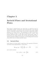
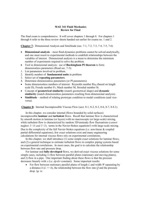
MAE 341 Fluid MechanicsReview for FinalThe final exam is comprehensive. It will cover chapters 1 through 8. For chapters 1through 6 refer to the three review sheets handed out earlier for exams no. 1 and 2.Chapter 7: Dimensional Analysis and Similitude (sec. 7-1, 7-2, 7-3, 7-4, 7-5, 7-6)• Dimensional analysis – most fluid-dynamics problems cannot be solved analytically,and one must resort to experimental methods to establish relationships between thevariables of interest. Dimensional analysis is a mean to determine the minimumnumber of experiments required to solve the problem.• Tool in dimensional analysis: use of Buckingham PI theorem to formdimensionless parameters (Read sec. 7-3):1. List parameters involved in problem.2. Identify number of fundamental units in problem3. Select set of repeating parameters.4. Determine dimensionless parameters (or PI parameters).• Some dimensionless numbers of interest: Reynolds number Re D (based on lengthscale D), Froude number Fr, Mach number M, Strouhal number St.• Concept of geometrical similarity (match geometrical shape) and dynamicsimilarity (match dimensionless parameters resulting from dimensional analysis).• Similitude – method of relating prototype condition to model conditions (and viceversa).Chapter 8: Internal Incompressible Viscous Flow (sect. 8-1, 8-2, 8-3, 8-6, 8-7, 8-8.1).In this chapter, we consider internal (flows bounded by solid surfaces)incompressible laminar and turbulent flows. Recall that laminar flow is characterizedby smooth motion in laminae (or layers) with no macroscopic (or large-scale) mixing,while turbulent flow is characterized by random 3D/unsteady flow fluctuations (cannotneglect / tand / x iterms in the Navier-Stokes equations!) with large-scale mixing.Due to the complexity of the full Navier-Stokes equations (i.e. non-linear & coupledpartial differential equations), few exact solutions exist and many engineeringcalculations for internal viscous flows rely on experimental correlations.In this chapter, we shall introduce (1) some simple exact solutions for laminar flows,and (2) a general technique to estimate turbulent flows in complex piping systems basedon experimental correlations. In most cases, the goal is to calculate the relationshipbetween flow rate and pressure drop.For laminar and fully-developed flows, we derived exact viscous solutions for somesimple cases, including 1) flow between parallel plates (stationary and moving plates),and 2) flow in a pipe. One important finding about these flows is that the pressuredecreases linearly with x (i.e. dp/dx=constant). Some important results:• For flow between stationary parallel plates of length L and width W separating bya distance h (L >> h), the relationship between the flow rate Q and the pressuredrop p is:

3Q h p=(8.6c)W 12µL• For flow between parallel plates (one stationary and one moving with speed U),we have:3Q Uh h dp= (8.9b)W 2 12µ dx• For flow in a pipe of diameter D, we have:D pQ = 4128 µL(8.13c)Using the abover result, we can express the head loss h lin terms of the frictionfactor f lamfor laminar flow as:2pL Vhl = flamwhere f lam= 64DVand Re =D 2ReµApplications of these exact solutions for laminar flows are limited to low Reynoldsnumber flows such as lubrication. Recall that the Reynolds number Re is a measure ofthe inertial force over the viscous force.For most applications, the flow is turbulent and no exact solution exists even forthe simplest geometry. We must resort to experimental correlations to tackle theseproblems. For flows in complex piping systems, the energy equation is employed. Ittakes on the form:22 p1V1 p2V2 + 1+ gz1 + 2+ gz2 = h lT(8.28) 2 2 where 1 1 and 2 1 (for turbulent flow), and h lTis the total head loss which isdetermined from experimental correlations. In general, the total head loss is expressed as222 L V L= +e , n VnVmhlTff + Km D 2 n D 2 m 2 where the first term on the RHS represents the major loss due to the straight pipesections, and the second term in parenthesis on the RHS represents the minor losses dueto pipe entrance, contraction/expansion sections, valves, elbows, bends, etc … Themajor loss is expressed in terms of the friction factor f which can be obtained from Fig.8.12 (pg. 339). In general, the friction factor is a function of the Reynolds number Reand the roughness ratio e/D. Figure 8.14 indicates that for rough pipes, the frictionfactor f is a weak function of Re. The minor losses weak functions of Re, and are oftenexpressed in terms of an “equivalent” pipe length L eor a loss coefficient K . Theseparameters are determined from tabulated tables and curves. Please read section 8-8 onhow to solve single-path pipe flow problems.Finally, if viscous loss is neglected, i.e. h lT =0, Eq. (8.28) reduces to the Bernoulliequation.

Chapter 9: External Incompressible Viscous Flow (sect. 9-1, 9-7).In this chapter, we consider external (flows over bodies immersed in an unboundedfluid) incompressible laminar and turbulent flows. The goal is to calculate the dragforce over the body. Again, due to the complexity of the governing flow equations (i.e.the Navier-Stokes equations), few exact solutions exist and many engineeringcalculations for viscous flows rely on experimental correlations. In this chapter, we shallintroduce (1) a simple exact solution to illustrate the difficulties associated with solvingthe Navier-Stokes equations, and (2) a general technique to estimate drag force overcomplex geometry based on experimental correlations.We first consider the flow over a stationary flat plate where we introduce theboundary-layer concept. Here, the flowfield is divided into two regions. Near thesurface, both viscous force and inertia force are important, and the velocity varies fromzero at the surface (due to the no-slip condition) to the freestream velocity at the edge ofthe region – the so-called boundary layer region. Outside the boundary layer region, theflow can be assumed inviscid – the so-called inviscid flow region. In a boundary-layerapproximation, we assume that the boundary layer thickness is thin. For laminar flow,it can be shown that the scaling of the boundary layer thickness is as follows: 1Ux where Rex12 /x RexµMost external-flow applications have “large” Reynolds numbers (Re >> 1). If the body isa streamlined body, the boundary layer approximation is very accurate (e.g. flow overan airfoil near the design condition). For bodies that are not streamlined (or bluffbodies), large separated region exist near the surface and the boundary layerapproximation does not apply here (e.g. flow over a cylinder).For laminar flow over a flat plate in the absence of a pressure gradient (i.e. thestatic pressure in the inviscid-flow region is constant), the Navier-Stokes equation can besolved analytically. The exact solution yields the following key results: 5UxBoundary layer thickness:= Re/x (9.13)12x RexµD 1328 .ULDrag coefficient:CD = Re/L(9.33)1122U AReLµ2where A is the total surface area in contact with the fluid. For a flat plate, A=LW whereL and W are the length and width of the flat plate, respectively. Note that the aboveresults are applicable in the range of roughly Re L 10 5 .As before, for turbulent flows, there exists no exact solution even for the simplestflow, and we must rely on experimental correlations to estimate drag force. Usingdimensional analysis, it is possible to tabulate test data for various geometries of practicalinterest (e.g. flat plate, cylinder, sphere, disk). In many cases, it can be shown that thedrag coefficient is at most a function of the Reynolds number.

For a flat plate, assuming fully turbulent flow over the flat plate, variouscorrelations for drag coefficient exist. One such correlation is (see also Fig. 9.8 on page5 7440 – valid for 5× 10 < Re L< 10 ): 0.382Boundary layer thickness:=x Re (9.26)15 /xD 0074 .Drag coefficient:CD =(9.34)1152U ARe /L2Note the difference in the scaling of C D with Re L between laminar flow (power 1/2) andturbulent flow (power 1/5). Using the above results, we see thatturb310 /CDturb,310 /= 0. 0764 Rex= 0. 0557 ReLClamDlam ,For a typical application in the turbulent flow regime with Re = 50 L. × 106 , the aboveresult shows that CD, turb/ CD,lam= 5.7 . Clearly, use of the laminar-flow result in theturbulent-flow regime would have underestimated the drag force by a factor of 5.7!For flows over bluff bodies, it turns out that the effect of Reynolds number isweak for many geometries, and the drag coefficient (usually normalized to the frontalarea A) is a constant over a wide range of Reynolds number of practical interest (e.g.Table 9.3 on page 443). For example, for a disk, the drag coefficient is C D =1.17 forRe D >10 3 (frontal area is D 2 / 4 ). The drag over some bluff-body geometries such as asphere (Fig. 9.11 on page 444) and a cylinder (Fig. 9.13 on page 446) does depend on theReynolds number.