Comparison between 1D and 2D models to analyze the dam break
Comparison between 1D and 2D models to analyze the dam break
Comparison between 1D and 2D models to analyze the dam break
- No tags were found...

You also want an ePaper? Increase the reach of your titles
YUMPU automatically turns print PDFs into web optimized ePapers that Google loves.
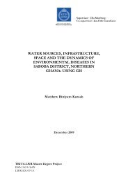
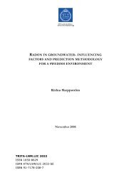
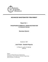
<strong>Comparison</strong> <strong>between</strong> <strong>1D</strong> <strong>and</strong> <strong>2D</strong> <strong>models</strong> <strong>to</strong> <strong>analyze</strong> <strong>the</strong> <strong>dam</strong> <strong>break</strong> waveABSTRACTThe simulation of exceptional events characterized by high hydraulic <strong>and</strong> hydro-geologic risk is an actual problem for<strong>the</strong> scientific community, working in <strong>the</strong> <strong>to</strong>pic of environmental protection. There have been around 200 notable<strong>dam</strong> <strong>and</strong> reservoir failures worldwide in <strong>the</strong> twentieth century. These failures have caused severe devastation in <strong>the</strong>valleys downstream both in terms of lives lost <strong>and</strong> widespread <strong>dam</strong>age <strong>to</strong> infrastructure <strong>and</strong> property.The flood wave caused by a <strong>dam</strong> failure can result in <strong>the</strong> loss of human lives <strong>and</strong> have a severe economic impact.Therefore, significant efforts have been carried out over <strong>the</strong> years <strong>to</strong> produce methods for determination of <strong>the</strong>extent <strong>and</strong> timing of <strong>the</strong> flood wave.This work describes <strong>and</strong> compares two <strong>models</strong> for solving <strong>the</strong> <strong>dam</strong> <strong>break</strong> problem using <strong>the</strong> FEM (finite elementmethod). Both <strong>models</strong> are based on solving <strong>the</strong> Shallow Water equations. The first model is one-dimensional <strong>and</strong> <strong>the</strong>second is two-dimensional.Most simulation studies for <strong>the</strong> <strong>dam</strong> <strong>break</strong> problem are currently attempted using one-dimensional <strong>models</strong>, <strong>and</strong> weinvestigate here <strong>the</strong> possibility of moving <strong>to</strong> two-dimensional simulations solving <strong>and</strong> comparing <strong>the</strong> two <strong>models</strong>with a finite element analysis <strong>and</strong> solver software package called Comsol Multiphysics.Comsol Multiphysics is a modelling package for <strong>the</strong> simulation of any physical process describable with partialdifferential equations (PDEs). The hydraulic analysis of <strong>the</strong> <strong>dam</strong> <strong>break</strong> problem from a different point of view hasbeen done in this work, that is, using a generic <strong>to</strong>ol not adapted <strong>to</strong> solve this kind of problems. This fact helps us <strong>to</strong>underst<strong>and</strong> <strong>the</strong> process entirely because of <strong>the</strong> necessity of introducing all <strong>the</strong> conditions <strong>and</strong> equations. We are ablein this way <strong>to</strong> control all <strong>the</strong> details within <strong>the</strong> model, even though we have o<strong>the</strong>r problems in relation with <strong>the</strong>generic nature of <strong>the</strong> program.A simple example of <strong>the</strong> collapse of a <strong>dam</strong> is used <strong>to</strong> demonstrate <strong>the</strong> capability of <strong>the</strong> two <strong>models</strong>. Theinstantaneous collapse over wet bed has been studied. Some difficulties are encountered simulating dry bed conditionfor <strong>the</strong> appearance of negative depths or velocity overshoots. The important influence of <strong>the</strong> bathymetry has beenalso demonstrated during <strong>the</strong> simulations.Key words: Shallow water equations; Dam-<strong>break</strong> simulation; Finite elements method; Bathymetry.1. - INTRODUCTION1.1 Literature review1.1.1 GeneralThe first law on <strong>dam</strong> safety was passed in France inMay 1968. Emergency plans had <strong>to</strong> be prepared forevery <strong>dam</strong> higher than 20 m <strong>and</strong> with a reservoirvolume over 15 Mm 3 . At that time, <strong>the</strong> numericalsimulation of <strong>dam</strong>-<strong>break</strong> problems could beaccomplished only with one-dimensional <strong>to</strong>ols <strong>and</strong>accordingly <strong>the</strong>se were used <strong>to</strong> predict <strong>the</strong> spreadof <strong>the</strong> flood wave (Hervouet 2000).Since 1994, however, new regulations havedem<strong>and</strong>ed an updating of existing emergency plansfor large <strong>dam</strong>s. Emergency Response Plans nowhave <strong>to</strong> be prepared by <strong>the</strong> local authority afterconsulting <strong>the</strong> relevant mayors <strong>and</strong> <strong>dam</strong> opera<strong>to</strong>rs.The scope of <strong>the</strong> Emergency Response Planincludes:1.- <strong>the</strong> identification of potential risks;2.- a list of protective measures <strong>and</strong> mechanisms <strong>to</strong>implement <strong>the</strong>m;3.- definition of <strong>the</strong> responsibilities of localgovernment agencies <strong>and</strong> o<strong>the</strong>r organizationsinvolved;4.- dissemination of information <strong>to</strong> <strong>the</strong> public;The <strong>dam</strong> opera<strong>to</strong>r is now required <strong>to</strong> carry out arisk assessment study which provides informationon <strong>the</strong> area covered by <strong>the</strong> Emergency ResponsePlan <strong>and</strong> which distinguishes <strong>between</strong>:1.- <strong>the</strong> near safety zone, flooded in less than 15 minafter <strong>the</strong> <strong>dam</strong>-<strong>break</strong>;2.- <strong>the</strong> remote flooded area. Since 1994, thisextends <strong>to</strong> <strong>the</strong> limit at which ‘<strong>the</strong>re is no danger for<strong>the</strong> population’.As a consequence of this new law, a risk analysis ofmany <strong>dam</strong>s must be completed. Although many of<strong>the</strong>se studies, particularly those relating <strong>to</strong>hydroelectric power stations in narrow upl<strong>and</strong>valleys, could be completed with a one-dimensionalprogram, a small but significant number ofproblems dem<strong>and</strong>ed a two-dimensional approach.These include flood waves spreading in largevalleys or those that ultimately reach <strong>the</strong> sea via aflat coastal plain. In both <strong>the</strong>se cases, widespread,<strong>and</strong> relatively shallow inundation results in a flowfield that is significantly <strong>1D</strong> in nature <strong>and</strong> which isamenable <strong>to</strong> simulation using <strong>the</strong> shallow water orSaint Venant equations. Given <strong>the</strong> complexity of<strong>dam</strong>-<strong>break</strong> hydraulics, it is also probable that more<strong>and</strong> more two-dimensional studies will have <strong>to</strong> becompleted in <strong>the</strong> future (Hervouet 2000).1.1.2 Review of numerical methods for <strong>dam</strong><strong>break</strong>.A brief review of <strong>the</strong> numerical methods used in1
Ignacio Valcárcel LencinaTRITA LWR Masters Thesis<strong>the</strong> <strong>dam</strong> <strong>break</strong> problem has been done, although itis not <strong>the</strong> objective of this work.Numerical simulation <strong>models</strong> are powerful <strong>to</strong>ols <strong>to</strong>assess <strong>the</strong> impact of floods due <strong>to</strong> <strong>dam</strong> failure events.Different codes are available for numerical simulationsof floods caused by <strong>dam</strong> failures.At present, classical methods <strong>and</strong> central differenceschemes dominate <strong>the</strong> software products for <strong>the</strong>shallow-water system of equations. Some years after<strong>the</strong>ir adoption for solving problems in gas dynamics,upwind schemes have been successfully used for <strong>the</strong>solution of <strong>the</strong> shallow water equations, with similaradvantages. His<strong>to</strong>rically, upwind schemes weredeveloped specifically for <strong>the</strong> solution of <strong>the</strong> Eulerequations, but <strong>the</strong>re is no reason why <strong>the</strong> techniquesinvolved cannot be applied for <strong>the</strong> solution of o<strong>the</strong>rsystems of conservation laws.First-order <strong>and</strong> second-order schemes have been used<strong>to</strong> solve two-dimensional <strong>dam</strong> <strong>break</strong> flows onstructured meshes following central differences <strong>and</strong>upwind flux difference approaches. More recently,first <strong>and</strong> second-order upwind schemes onunstructured meshes have been presented for this kindof flow.Besides this, discussion is open as <strong>to</strong> whe<strong>the</strong>r <strong>the</strong>schemes based on one-dimensional Riemann solversare <strong>the</strong> most suitable choice for multi-dimensionalcalculations because <strong>the</strong>y seem inadequate forcapturing two-dimensional flow features. Multidimensionalupwinding techniques have demonstrated<strong>to</strong> give very good resolution for <strong>dam</strong> <strong>break</strong> problemsin genuinely two-dimensional domains, but <strong>the</strong>irimplementation is more complicated.1.1.3 Hydraulic flow <strong>models</strong> available for <strong>dam</strong> <strong>break</strong>flood simulations.Some flow <strong>models</strong> available for <strong>dam</strong> <strong>break</strong> flowsimulation are listed in table 1 (ICOLD, 1999).1.1.4 FEM, FVM or FDM?Several techniques are available in literature, <strong>to</strong> solve<strong>the</strong> two-dimensional shallow water equations for <strong>the</strong>simulation of free-surface flows transients. Theseinclude finite difference methods (FDM), finiteelement methods (FEM) <strong>and</strong> <strong>the</strong> finite volumemethods (FVM) (Valiani et al 1999).Table 1. Some flow <strong>models</strong> for <strong>dam</strong>-<strong>break</strong> flood simulations (ICOLD, 1999). (*<strong>2D</strong> <strong>models</strong>)AgencyName of <strong>models</strong>1 USA / National Wea<strong>the</strong>r Service DAMBRK (original)2 USA / National Wea<strong>the</strong>r Service SMPDBK (Simpified Dam<strong>break</strong>)3 BOSS International BOSS DAMBRK4 HAESTED METHODS HAESTED DAMBRK5 Binnie & Partners UKDAMBRK6 Department of Water Affairs <strong>and</strong> Foresty Pre<strong>to</strong>ria, DWAF-DAMBRK7 USA / COE- Hyrdologic Engineering Center HEC-programs (HEC-RAS)8 Tams LATIS9 (IWHR), PR China DBK 110 (IWHR), PR China *DBK 211 Royal Institute of Technology, S<strong>to</strong>ckholm TVDDAM <strong>and</strong> *COMSOL12 Cemagref RUBAR 313 Cemagref * RUBAR 2014 Cemagref CASTOR15 Delft Hydraulics SOBEK16 Delft Hydraulics *DELFT 2 D17 Consulting Engineers Reiter Ltd. DYX 1018 ANU-Reiter Ltd. DYNET - ANUFLOOD19 ENEL Centro di Ricerca Idraulica RECAS20 ENEL Centro di Ricerca Idraulica *FLOOD <strong>2D</strong>21 ENEL Centro di Ricerca Idraulica STREAM22 Danish Hydraulic Institute MIKE 1123 Danish Hydraulic Institute *MIKE 2124 ETH Zürich FLORIS25 ETH Zürich *<strong>2D</strong>-MB26 EDF - Ladora<strong>to</strong>ire National Hydraulique RUPTURE27 EDF - Ladora<strong>to</strong>ire National Hydraulique *TELEMAC-<strong>2D</strong>2
<strong>Comparison</strong> <strong>between</strong> <strong>1D</strong> <strong>and</strong> <strong>2D</strong> <strong>models</strong> <strong>to</strong> <strong>analyze</strong> <strong>the</strong> <strong>dam</strong> <strong>break</strong> waveA finite element method (FEM) discretization is basedupon a piecewise representation of <strong>the</strong> solution interms of specified basis functions. The computationaldomain is divided up in<strong>to</strong> smaller domains (finiteelements) <strong>and</strong> <strong>the</strong> solution in each element isconstructed from <strong>the</strong> basis functions. The actualequations that are solved are typically obtained byrestating <strong>the</strong> conservation equation in weak form: <strong>the</strong>field variables are written in terms of <strong>the</strong> basisfunctions, <strong>the</strong> equation is multiplied by appropriatetest functions, <strong>and</strong> <strong>the</strong>n integrated over an element.Since <strong>the</strong> FEM solution is in terms of specific basisfunctions, a great deal more is known about <strong>the</strong>solution than for ei<strong>the</strong>r FDM or FVM. This can be adouble-edged sword, as <strong>the</strong> choice of basis functionsis very important <strong>and</strong> boundary conditions may bemore difficult <strong>to</strong> formulate. Again, a system ofequations is obtained (usually for nodal values) thatmust be solved <strong>to</strong> obtain a solution.<strong>Comparison</strong> of <strong>the</strong> three methods is difficult, primarilydue <strong>to</strong> <strong>the</strong> many variations of all three methods. FVM<strong>and</strong> FDM provide discrete solutions, while FEMprovides a continuous (up <strong>to</strong> a point) solution. FVM<strong>and</strong> FDM are generally considered easier <strong>to</strong> programthan FEM, but opinions vary on this point. FVM aregenerally expected <strong>to</strong> provide better conservationproperties, but opinions vary on this point also. Theimplementation of <strong>the</strong> model is based on <strong>the</strong>commercial FEM package Comsol Multiphysics,which reduces <strong>the</strong> programming effort required <strong>to</strong> aminimum.1.1.5 Numerical problems of <strong>the</strong> Shallow WaterEquations.The numerical solution of <strong>the</strong> shallow water equationsfor flood waves propagation over real domains posesthree specific problems, (Valiani et al 1999).The first problem is <strong>the</strong> simulation of <strong>the</strong> fronts orabrupt water waves that can be representednumerically as a propagating discontinuity. Thisproblem can be considered as solved since <strong>the</strong> lateeighties or early nineties.The second problem derives from abrupt changes inbathymetry. As long as <strong>the</strong> bot<strong>to</strong>m surface remainssufficiently smooth, most numerical techniquesprovide an accurate solution of <strong>the</strong> flow, but if <strong>the</strong>bot<strong>to</strong>m surface is very rough <strong>the</strong> majority of methodsfail.The last problem especially arises when <strong>the</strong>se schemesare applied <strong>to</strong> study <strong>the</strong> wave front propagation overdry bed. In fact, during <strong>the</strong> simulations of this work, aswe said before, some difficulties are encounteredsimulating dry bed condition for <strong>the</strong> appearance ofnegative depths or velocity overshoots; <strong>the</strong>refore, ourprincipal focus has been <strong>the</strong> wet case.To study <strong>the</strong> wave over dry bed is necessary <strong>to</strong> find asuitable numerical scheme (which is not <strong>the</strong> case ofComsol) that can efficiently <strong>and</strong> accurately simulate<strong>the</strong> flow with all its characteristics <strong>and</strong> features (using<strong>the</strong> two-step Taylor-Galerkin method, just <strong>to</strong> mentionone).Fur<strong>the</strong>rmore, is <strong>the</strong> hyperbolic character of <strong>the</strong>shallow water equations that makes finding solutions<strong>to</strong> <strong>the</strong>se equations difficult. Hyperbolic equationsadmit discontinuous as well as smooth or classicalsolutions. Even for <strong>the</strong> case in which <strong>the</strong> initial data issmooth, <strong>the</strong> non-linear character combined with <strong>the</strong>hyperbolic type of <strong>the</strong> initial of <strong>the</strong> equations can lead<strong>to</strong> discontinuous solutions in finite time.The non-linear character of <strong>the</strong> equations also meansthat analytical solutions <strong>to</strong> <strong>the</strong>se equations are limited<strong>to</strong> only very special cases. Numerical methods must beused <strong>to</strong> obtain solutions <strong>to</strong> practical problems.Therefore, numerical techniques which admitdiscontinuities in <strong>the</strong> solution, secondary shocks,reflections of waves, dry bed <strong>and</strong> obstructions arenecessary for <strong>the</strong> solution of <strong>the</strong> shallow waterequations. The method of characteristics, finitedifferences, finite elements <strong>and</strong> Godunov-typeschemes can be used <strong>to</strong> solve <strong>the</strong> shallow waterequations (Zoppou <strong>and</strong> Roberts 1991).1.2 Objectives of <strong>the</strong> study.The main objective of this work is <strong>to</strong> study <strong>and</strong>underst<strong>and</strong> <strong>the</strong> hydraulic analysis of <strong>the</strong> <strong>dam</strong>-<strong>break</strong>problem through <strong>the</strong> shallow water equations, solving<strong>the</strong>m from a different point of view, which is using ageneric <strong>to</strong>ol based on <strong>the</strong> FEM. Comparing both onedimensional<strong>and</strong> two-dimensional approaches, weunderst<strong>and</strong> entirely <strong>the</strong> whole process <strong>and</strong> we are able<strong>to</strong> answer some old questions about <strong>the</strong> benefit ofusing <strong>the</strong> <strong>1D</strong> or <strong>the</strong> <strong>2D</strong> model.Through simulation of two different <strong>models</strong>, we wish<strong>to</strong> achieve <strong>the</strong> following goals:- study <strong>the</strong> capacity of a particular general purpose <strong>2D</strong><strong>to</strong>ol <strong>to</strong> deal with <strong>dam</strong>-<strong>break</strong> simulations- compare simulation results of <strong>1D</strong> <strong>and</strong> <strong>2D</strong>simulations for comparable conditions- set a “point of reference” for <strong>2D</strong> computations.2. - GOVERNING EQUATIONS2.1 Navier-S<strong>to</strong>kes or Shallow Water Equations.Before describing <strong>the</strong> shallow water equations, it needs<strong>to</strong> be specified that <strong>the</strong>se are not <strong>the</strong> only equationsused <strong>to</strong> solve <strong>the</strong> <strong>dam</strong>-<strong>break</strong> problem. Therefore,using <strong>the</strong> approach (Quecedo et al 2004), where <strong>the</strong>authors compared two ma<strong>the</strong>matical <strong>models</strong> forsolving <strong>the</strong> <strong>dam</strong>-<strong>break</strong> problem, <strong>the</strong> Navier-S<strong>to</strong>kesequations are also a possible c<strong>and</strong>idate.As in many engineering problems, simulation of <strong>dam</strong><strong>break</strong> can be done with alternative ma<strong>the</strong>matical <strong>and</strong>numerical <strong>models</strong> with different levels ofapproximation. Quecedo compared two methodsbased on (i) solving <strong>the</strong> Navier–S<strong>to</strong>kes equations <strong>and</strong>(ii) using a depth integrated model which is discretizedusing a Taylor–Galerkin scheme. These ma<strong>the</strong>matical<strong>models</strong> are based on assumptions such as disregarding3
Ignacio Valcárcel LencinaTRITA LWR Masters Thesisair trapping in <strong>the</strong> former or vertical accelerations on<strong>the</strong> latter, <strong>and</strong> <strong>the</strong>ir range of application depends on<strong>the</strong>m.The validity of <strong>the</strong> shallow water approach was basedon comparisons of <strong>the</strong> model against problems with aknown analytical solution, which has been done bymany researchers over <strong>the</strong> past years.Concerning comparisons with in situ measurements,Quecedo applied <strong>the</strong> shalow water approach <strong>to</strong>simulate <strong>break</strong>ing of a tailing <strong>dam</strong> in East Texas. All<strong>the</strong>se comparisons do not concentrate on intervalswhere vertical accelerations are important, like <strong>the</strong>initial instants following failure, or <strong>the</strong> interaction withobstacles like vertical dykes. In <strong>the</strong>se cases, <strong>the</strong> errorscan be important.Quecedo used a more accurate approach <strong>to</strong> assess <strong>the</strong>validity of <strong>the</strong> shallow water approach in <strong>the</strong>se casesfor which no known analytical solutions are available.Based on <strong>the</strong> results obtained, <strong>the</strong> authors concludedthat:(i) The shallow water approach predicts (i) faster floodwaves when propagating over dry beds, thus providingsafer predictions of flood wave arrival times, (ii)reasonable estimations of <strong>the</strong> evolution of water depthfar from <strong>the</strong> <strong>dam</strong>.(ii) If failure takes place on<strong>to</strong> a wet bed, <strong>the</strong> shallowwater results can be considered reasonable incomparison <strong>to</strong> those obtained using <strong>the</strong> Navier–S<strong>to</strong>kesapproach.(iii) If <strong>the</strong> free surface curvature is high, <strong>the</strong> shallowwater approach misspredicts <strong>the</strong> pressure. Thus, itshould not be used <strong>to</strong> calculate, for instance, stresseson structures.In spite of <strong>the</strong> shortcomings of <strong>the</strong> shallow waterapproach when applied <strong>to</strong> <strong>dam</strong> <strong>break</strong> problems, <strong>the</strong>computational effort required by o<strong>the</strong>r methods, suchas <strong>the</strong> Navier–S<strong>to</strong>kes Level-Set algorithm presentedherein, in actual problems makes <strong>the</strong> shallow waterapproach attractive for large computational domains.The Navier–S<strong>to</strong>kes approach would be used for <strong>the</strong>analyses of small areas when knowledge of <strong>the</strong> threedimensionalstructure of <strong>the</strong> flow is needed.2.2 One-dimensional Shallow Water equations.Once we have seen that <strong>the</strong> shallow water equations(from now on “SWE”) are <strong>the</strong> most suitable <strong>to</strong>describe <strong>the</strong> <strong>dam</strong> <strong>break</strong> problem, <strong>the</strong> next step is <strong>to</strong>describe <strong>the</strong>m for <strong>the</strong> one-dimensional approach.The SWE are frequently used for modelling bothoceanographic <strong>and</strong> atmospheric fluid flow. Models ofsuch systems lead <strong>to</strong> <strong>the</strong> prediction of areas eventuallyaffected by pollution, coastal erosion, <strong>and</strong> polar icecapmelting.As previously seen in [2.1], comprehensive modellingof <strong>the</strong> <strong>dam</strong> <strong>break</strong> using physical descriptions such as<strong>the</strong> Navier-S<strong>to</strong>kes equations can often be problematic,due <strong>to</strong> <strong>the</strong> scale of <strong>the</strong> modeling domains. The SWE,of which <strong>the</strong>re are a number of representations,provide an easier description of such phenomena.The SWE are obtained from <strong>the</strong> Navier-S<strong>to</strong>kesequations, assuming that vertical velocities <strong>and</strong>accelerations are negligible <strong>and</strong> integrating over <strong>the</strong>water depth.This <strong>1D</strong> model investigates <strong>the</strong> settling of <strong>the</strong> <strong>dam</strong><strong>break</strong>wave over a variable bed as a function of time.A ma<strong>the</strong>matical relation represents <strong>the</strong> shape of <strong>the</strong>bed so that is easy <strong>to</strong> change parameters.The <strong>1D</strong> Saint-Venant’s-SWE are <strong>the</strong> following:∂z∂(zv)+ = 0∂t∂x2∂(zv)∂(zv ) ∂z∂zf+ + g ⋅ z ⋅ + g ⋅ z ⋅∂t∂x∂x∂x22∂ ( zv)∂ ( zv)−υc⋅ + g ⋅ z ⋅ Sf − E ⋅ = 022∂x∂xOr in <strong>the</strong> compact form:∂z+ ∇ ⋅ ( zv)= 0∂t∂(zv)T+ ∇ ⋅ ( zvv ) + g ⋅ z ⋅∇zS∂t−υ⋅ ∆(zv)+ g ⋅ z ⋅ Sf − E ⋅ ∆(zv)= 0cWhere z is <strong>the</strong> thickness of <strong>the</strong> water layer (m), v is <strong>the</strong>velocity (ms -1 ), g <strong>the</strong> gravity constant (m s –2 ), Sf is <strong>the</strong>friction term (explained later) <strong>and</strong> υ c <strong>the</strong> kinematicviscosity (m 2 s -1 ). The wind effect is not present in<strong>the</strong> equations.The dispersion coefficient E has been set <strong>to</strong> 2 m 2 /s.This value takes in<strong>to</strong> account <strong>the</strong> turbulence <strong>and</strong> <strong>the</strong>heterogeneity of <strong>the</strong> velocity on <strong>the</strong> vertical. It is amajor unknown in <strong>the</strong> case of <strong>dam</strong> <strong>break</strong>, but <strong>the</strong>results that we will see later, show that ComsolMultiphysics has need of artificial diffusion forstabilizing its solution.The definition of <strong>the</strong> thickness of <strong>the</strong> water layer, z, isz s -z f , where z s <strong>and</strong> z f are <strong>the</strong> measures in figure 1.(1)(2)(3)(4)4
<strong>Comparison</strong> <strong>between</strong> <strong>1D</strong> <strong>and</strong> <strong>2D</strong> <strong>models</strong> <strong>to</strong> <strong>analyze</strong> <strong>the</strong> <strong>dam</strong> <strong>break</strong> waveFigure 1. Representative vertical section through <strong>the</strong> fluiddomain showing <strong>the</strong> bed of a lake <strong>and</strong> <strong>the</strong> water surface.2.3 Two-dimensional Shallow Water equations.Depth averaging of <strong>the</strong> free surface flow equationsunder <strong>the</strong> shallow water hypo<strong>the</strong>sis leads <strong>to</strong> a commonversion of <strong>the</strong> two dimensional SWE, wich inconservative form is:∂z∂(zu)∂(zv)+ + = 0∂t∂x∂y∂(zu)∂(zu+∂t∂x2) ∂(zuv)+∂y(5)∂z∂zf (6)− f ⋅ zv + g ⋅ z ⋅ + g ⋅ z ⋅∂x∂x22∂ ( zu)∂ ( zu)+ g ⋅ z ⋅ Sfx− E ⋅ − E ⋅ = 022∂x∂y∂(zv)∂(zuv)∂(zv+ +∂t∂x∂y+ g ⋅ z ⋅ Sf2)∂z∂zf (7)+ f ⋅ zu + g ⋅ z ⋅ + g ⋅ z ⋅∂y∂yy22∂ ( zv)∂ ( zv)− E ⋅ − E ⋅ = 022∂x∂yThe equations above are valid under <strong>the</strong> followingassumptions:1. The fluid is well-mixed vertically with a hydrostaticpressure gradient.2. The density of <strong>the</strong> fluid is constant.3. We study water waves of long wave lengths.4. The viscosity term is negligible.Where z is <strong>the</strong> depth of water, zu <strong>and</strong> zv are unitdischarges along <strong>the</strong> co-ordinate directions. Inaddition, u <strong>and</strong> v are <strong>the</strong> velocities in <strong>the</strong> x <strong>and</strong> ydirections respectively, g is <strong>the</strong> acceleration due <strong>to</strong>gravity <strong>and</strong> Sf x <strong>and</strong> Sf y are <strong>the</strong> friction terms in <strong>the</strong> x<strong>and</strong> y directions respectively. The turbulent dissipationterms (E) <strong>and</strong> Coriolis effect (f) are present in <strong>the</strong>equations, but not <strong>the</strong> wind effect, which is notsignificant in <strong>the</strong> usual valleys where <strong>the</strong> <strong>dam</strong>-<strong>break</strong>occurs.2.3.1 The friction term.Many two-dimensional depth-averaged <strong>models</strong> includeonly friction at <strong>the</strong> bot<strong>to</strong>m. Specifically, <strong>models</strong> thatassume vertical channel side-walls <strong>and</strong> use free-slipboundary conditions do not account for <strong>the</strong> friction at<strong>the</strong> walls. Neglecting this effect, open channel flowwould likely show a marked variation in water depthfrom <strong>the</strong> one measured experimentally.Evaluation of <strong>the</strong> friction slope that quantifies <strong>the</strong>energy loss at <strong>the</strong> side-walls of <strong>the</strong> channel is required.It is common <strong>to</strong> use a uniform flow law, Manning orChezy formulae, <strong>to</strong> calculate this term. However, <strong>the</strong>selaws were developed for one-dimensional flow <strong>and</strong>must be extended <strong>and</strong> properly incorporated <strong>to</strong> twodimensionalequations.Manning’s formula used in one-dimensional shallowwater<strong>models</strong> is expressed in <strong>the</strong> formSfn2A⋅ Q ⋅ Q= (8)2⋅ R4 / 3Where n is <strong>the</strong> Manning coefficient <strong>and</strong> R = A/P is <strong>the</strong>hydraulic radius, which depends on <strong>the</strong> wettedperimeter P. For a rectangular channel P = b + 2z<strong>and</strong> for an irregular basin P = b.A distinction must be made <strong>between</strong> an arbitrarychannel cross-section <strong>and</strong> a cross-section with verticalwalls (fig. 2). Most two-dimensional <strong>models</strong> assumevertical walls <strong>and</strong> free-slip wall boundary conditionsfor rectangular channels, while <strong>the</strong> equations used <strong>to</strong>compute <strong>the</strong> friction term are based on irregular crosssections.To correct this inconsistency, <strong>the</strong> frictionslope equation has been modified here <strong>to</strong> reflect <strong>the</strong>vertical side-wall assumption. Basically, <strong>the</strong>modification ensures that <strong>the</strong> entire wetted perimeter(bot<strong>to</strong>m width <strong>and</strong> side-walls) is accounted for.For an arbitrary cross-section, <strong>the</strong> wetted perimeter ina cell is equal <strong>to</strong> <strong>the</strong> bot<strong>to</strong>m width b (fig. 2), so that <strong>the</strong>hydraulic radius adopts <strong>the</strong> form R = z, <strong>the</strong> waterdepth. In this case, <strong>the</strong> two-dimensional friction termsare written in <strong>the</strong> form (Brufau <strong>and</strong> García-Navarro2000):22n ⋅ u ⋅ u +Sf x 4/ 3zv2= (9)22n ⋅ v ⋅ u +Sf y 4 / 3zv2= (10)5
Ignacio Valcárcel LencinaTRITA LWR Masters ThesisFigure 2. Irregular <strong>and</strong> rectangular cross sections.3. - MO DEL L I N G THE <strong>1D</strong> DAM-BREAKWAVE.3.1 Assumptions.The basic assumption is that a failure <strong>and</strong> <strong>the</strong> resultingflood wave can reasonably be modeled using analyticaltechniques. Existing computer <strong>models</strong> have been used<strong>to</strong> recreate actual failures with a close representation <strong>to</strong>observed crests. However, unrealistic results can beobtained without a careful analysis.In this model, it has been assumed that <strong>the</strong> <strong>dam</strong> failedcompletely <strong>and</strong> instantaneously.This ‘main’ assumption of instantaneous <strong>and</strong> completebreach (<strong>the</strong> breach is <strong>the</strong> opening formed in <strong>the</strong> <strong>dam</strong>when it fails) was used for reasons of conveniencewhen applying certain ma<strong>the</strong>matical techniques foranalysing <strong>dam</strong>-<strong>break</strong> flood waves. The presumptionsare somewhat appropriate for concrete arch-type<strong>dam</strong>s, but <strong>the</strong>y are not suitable for ear<strong>the</strong>n <strong>dam</strong>s <strong>and</strong>concrete gravity-type <strong>dam</strong>s.● Ear<strong>the</strong>n <strong>dam</strong>s, which exceedingly outnumber allo<strong>the</strong>r types of <strong>dam</strong>s, do not tend <strong>to</strong> completely fail,nor do <strong>the</strong>y fail instantaneously. Once a developingbreach has been initiated, <strong>the</strong> discharging water willerode <strong>the</strong> breach until ei<strong>the</strong>r <strong>the</strong> reservoir water isdepleted or <strong>the</strong> breach resists fur<strong>the</strong>r erosion. Thefully formed breach in ear<strong>the</strong>n <strong>dam</strong>s tends <strong>to</strong> have anaverage width (b) in <strong>the</strong> range (h d
<strong>Comparison</strong> <strong>between</strong> <strong>1D</strong> <strong>and</strong> <strong>2D</strong> <strong>models</strong> <strong>to</strong> <strong>analyze</strong> <strong>the</strong> <strong>dam</strong> <strong>break</strong> waveTo conclude, <strong>the</strong> last assumption concerns about <strong>the</strong>bathymetry profiling. An unreal bathymetry has beengenerated for <strong>the</strong> <strong>1D</strong> model by <strong>the</strong> function sin(x)/10,which have been developed only downstream of <strong>the</strong><strong>dam</strong>, where it has <strong>the</strong> real influence.This function creates a group of small elevations of±10 cm downstream of <strong>the</strong> <strong>dam</strong>, in order <strong>to</strong> observe<strong>the</strong> big influence of <strong>the</strong> bathymetry profiling when <strong>the</strong><strong>dam</strong> <strong>break</strong> wave sweep along <strong>the</strong> valley. In <strong>the</strong>denomina<strong>to</strong>r of <strong>the</strong> function <strong>the</strong>re is a 10, it has beenonly <strong>the</strong> result after some different tests <strong>to</strong> prove <strong>the</strong>most suitable profile for <strong>the</strong> simulations.3.2 Dependent variables.Our dependent variables for this <strong>1D</strong> model are z <strong>and</strong>zv. Where z is <strong>the</strong> depth of water, <strong>and</strong> zv is <strong>the</strong> unitdischarge along <strong>the</strong> co-ordinate direction.3.3 Constants.In this model, we call ‘constants’ <strong>the</strong> variables that areindependent of <strong>the</strong> geometry. Constants are global,that is, <strong>the</strong>y are <strong>the</strong> same for all geometries <strong>and</strong>subdomains. In this <strong>1D</strong> model <strong>the</strong> following constantshave been used:Kinematic viscosity: ν = µ / ρIt is expressed as <strong>the</strong> dynamic viscosity divided by <strong>the</strong>density of <strong>the</strong> fluid. Kinematic viscosity is a measureof <strong>the</strong> resistive flow of a fluid under <strong>the</strong> influence ofgravity. Kinematic viscosity (Greek symbol nu: ν c ) hasSI units (m 2 s -1 ). The kinematic viscosity of water at20ºC is 10 -6 m 2 /s, <strong>and</strong> that is <strong>the</strong> value we assume forour model. This viscosity term is negligible; it has noinfluence although is has been taken in<strong>to</strong>consideration. In <strong>the</strong> <strong>2D</strong> model, <strong>the</strong> viscosity term isneglected <strong>and</strong> this is not an imprecise assumption.Acceleration due <strong>to</strong> gravityAt <strong>the</strong> Earth's surface, denoted g, is approximately 9.8m/s 2 (meters per second squared).Eddy diffusion coefficientIn fluid dynamics, an ‘eddy’ is <strong>the</strong> swirling of a fluid<strong>and</strong> <strong>the</strong> reverse current created when <strong>the</strong> fluid flowspast an obstacle. The moving fluid creates a spacedevoid of downstream-flowing water on <strong>the</strong>downstream side of <strong>the</strong> object. Fluid behind <strong>the</strong>obstacle flows in<strong>to</strong> <strong>the</strong> void creating a swirl of fluid oneach edge of <strong>the</strong> obstacle, followed by a short reverseflow of fluid behind <strong>the</strong> obstacle flowing upstream,<strong>to</strong>ward <strong>the</strong> back of <strong>the</strong> obstacle. This phenomenon ismost visible behind large emergent rocks in swiftflowingrivers.The ‘eddy diffusivity’ is <strong>the</strong> exchange coefficient for<strong>the</strong> diffusion of a conservative property by eddies in aturbulent flow. Also known as eddy-diffusioncoefficient. In this model, this coefficient is relevant <strong>to</strong>get <strong>the</strong> stability in <strong>the</strong> simulations. Without thiscoefficient, <strong>the</strong> results have been not satisfac<strong>to</strong>ry at all.We need this artificial diffusion for stabilizing <strong>the</strong>solution. The dispersion coefficient E has been set <strong>to</strong>2 m 2 /s.Manning's Roughness CoefficientRoughness coefficients represent <strong>the</strong> resistance <strong>to</strong>flood flows in channels <strong>and</strong> flood plains. Suggestedvalues for Manning's n, tabulated according <strong>to</strong> fac<strong>to</strong>rsthat affect roughness, are found in <strong>the</strong> literature.Roughness characteristics of natural channels are givenby Barnes (1967). Barnes presents pho<strong>to</strong>graphs <strong>and</strong>cross sections of typical rivers <strong>and</strong> creeks <strong>and</strong> <strong>the</strong>irrespective n values. From <strong>the</strong>se guides we fetch atypical value for flood plains, n = 0.025Figure 3. The Constants dialog box.3.4 Scalar expressions.The scalar expressions are used <strong>to</strong> define scalarexpression variables that are valid on all geometrylevels everywhere in <strong>the</strong> current geometry. Thefollowing expressions have been defined in <strong>the</strong> model:The bed profile z f has been defined in this way:z f = (0)*(x=52)This is <strong>the</strong> analytical expression that has been chosen<strong>to</strong> define <strong>the</strong> bathymetry in <strong>the</strong> <strong>1D</strong> model; it meansthat <strong>the</strong>re is a flat bed profile <strong>the</strong> first 52 m (upstreamof <strong>the</strong> <strong>dam</strong>) <strong>and</strong> a ‘sinusoidal’ bed profile downstreamof <strong>the</strong> <strong>dam</strong>, that is, <strong>the</strong> last 48 m of <strong>the</strong> one hundredmetres-domain.The derivative of z f with respect <strong>to</strong> <strong>the</strong> variable x hasbeen introduced here for computational effortreasons. Computing this term apart, <strong>the</strong> computerdoes not need <strong>to</strong> do it in <strong>the</strong> simulation for every finiteelement of <strong>the</strong> mesh, it takes simply <strong>the</strong> value which issaved here as ano<strong>the</strong>r expression. This term appears in<strong>the</strong> equations as we saw in [2.2].The initial value of <strong>the</strong> water layer z 0 has been set in<strong>the</strong> same way as <strong>the</strong> bed profile, that is: z 0 =(10)*(x=50). It is developed in detail in[3.7].The friction term seen in [2.3.1] has been introducedhere with a different expression but it is really <strong>the</strong>same. All <strong>the</strong> expressions as possible have been setapart from <strong>the</strong> equations for own convenience <strong>and</strong>computational effort reasons.7
Ignacio Valcárcel LencinaTRITA LWR Masters ThesisFigure 4. The Scalar Expressions dialog box.3.5 Geometry.To create <strong>the</strong> <strong>1D</strong> geometry model, a line which is 100m in length has been drawn. This is <strong>the</strong> first step <strong>to</strong> doonce <strong>the</strong> dimensions <strong>and</strong> <strong>the</strong> dependant variables havebeen chosen. The figure below show <strong>the</strong> <strong>1D</strong> geometrymodel:Figure 6. Bathymetry profile, z f , used in <strong>the</strong> model.Figure 7. The initial water surface profile <strong>and</strong> <strong>the</strong>bathymetry profileFigure 5. <strong>1D</strong> geometry model3.6 Bathymetry profile.As it was written previously, <strong>the</strong> bed profile z f hasbeen defined in this way:z f = (0)*(x=52)In <strong>the</strong> figure below we can see <strong>the</strong> sinusoidal bedprofile only downstream of <strong>the</strong> <strong>dam</strong>, <strong>the</strong> zone ofinterest for us hydrodynamically speaking (notice <strong>the</strong>difference in scale <strong>between</strong> <strong>the</strong> x <strong>and</strong> y direction). Thiskind of profile is <strong>the</strong>oretical, but <strong>the</strong> purpose here isshowing <strong>the</strong> influence of <strong>the</strong> <strong>to</strong>pography of <strong>the</strong> bed on<strong>the</strong> elevation of <strong>the</strong> water surface. To see thisinfluence, <strong>the</strong>se small elevations of 10 cm have beenintroduced. A higher elevation profile has moreinfluence on <strong>the</strong> water surface, but it introduces muchmore instabilities in <strong>the</strong> model.3.7 Initial value.For a time-dependent analysis, initial conditions mustbe provided. An initial value for each dependentvariable is entered. We can also enter initial values for<strong>the</strong> first time derivative of <strong>the</strong> dependent variables.These are used when solving time-dependentproblems containing second time derivatives. In thiscase <strong>the</strong>re are no second time derivatives, <strong>the</strong>n weenter zero in both edit fields.Only one value different from zero in <strong>the</strong> first editfield is entered, for <strong>the</strong> dependent variable z. Thisvalue is equal <strong>to</strong> z 0 because it was defined previously in<strong>the</strong> scalar expressions [3.4]. At t=0 <strong>the</strong> value of <strong>the</strong>o<strong>the</strong>r dependent variable zv is equal <strong>to</strong> zero.The figure 7 above shows clearly <strong>the</strong> situation at t = 0,before <strong>the</strong> <strong>dam</strong> <strong>break</strong> occurs.The expression for <strong>the</strong> initial value is:z 0 = (10)*(x=50).8
<strong>Comparison</strong> <strong>between</strong> <strong>1D</strong> <strong>and</strong> <strong>2D</strong> <strong>models</strong> <strong>to</strong> <strong>analyze</strong> <strong>the</strong> <strong>dam</strong> <strong>break</strong> waveIn <strong>1D</strong>, Comsol Multiphysics always uses regularrefinement, where it divides each element in<strong>to</strong> twoelements of <strong>the</strong> same shape. The refinement of <strong>the</strong>mesh has gone from 15 <strong>to</strong> 7680 elements, <strong>the</strong> finaldivision that has been chosen <strong>to</strong> define <strong>the</strong> model withan acceptable accuracy.Figure 8. The initial condition specification page in <strong>the</strong>Subdomain Settings dialog box.3.8 Meshing.A mesh is a partition of <strong>the</strong> geometric model in<strong>to</strong>small units of simple shape. For <strong>1D</strong> geometry <strong>the</strong>software partitions <strong>the</strong> subdomains (intervals) in<strong>to</strong>smaller intervals (or mesh elements). The endpoints of<strong>the</strong> mesh elements are called ‘mesh vertices’.The value in <strong>the</strong> ‘Maximum element size’ edit fieldspecifies <strong>the</strong> maximum allowed element size, which bydefault is 1/15th of <strong>the</strong> size of <strong>the</strong> geometry.The value in <strong>the</strong> ‘Maximum element size scalingfac<strong>to</strong>r’ edit field comes in<strong>to</strong> play if we do not explicitlygive a maximum element size. In that case, <strong>the</strong>software multiplies <strong>the</strong> default maximum element sizeby this fac<strong>to</strong>r; its default value is 1.The value in <strong>the</strong> ‘Element growth rate’ edit fielddetermines <strong>the</strong> maximum rate at which <strong>the</strong> elementsize can grow from a region with small elements <strong>to</strong> aregion with larger elements. The value must be greateror equal <strong>to</strong> one. The default value is 1.3, that is,element size can grow by 30% (approximately) fromone element <strong>to</strong> ano<strong>the</strong>r.Table 2. Mesh parameters <strong>and</strong> statistics.ParameterMaximum element size 1Maximum element size scaling fac<strong>to</strong>r 1ValueElement growth rate 1.3X-direction scale fac<strong>to</strong>r 1.0Number of degrees of freedom 30722Number of elements 76803.9 Subdomain settings.The subdomain settings describe <strong>the</strong> physics on amodel’s main domain, which is divided in<strong>to</strong>subdomains. In this model, <strong>the</strong>re is only onesubdomain.The PDE in its general form is used with a timedependent analysis. The PDE in <strong>the</strong> general form has<strong>the</strong> following aspect in <strong>the</strong> program:e2∂ u+ d∂t∂u⋅ + ∇ ⋅ Γ∂ta⋅a=2F(11)The next step is <strong>to</strong> introduce <strong>the</strong> equations seen in[2.2] adapting <strong>the</strong>m <strong>to</strong> this general form, that is, <strong>the</strong><strong>1D</strong>-SWE must be introduced in <strong>the</strong> proper formatthat Comsol Multiphysics requires.Figure 9. The flux vec<strong>to</strong>r edit fieldWhen trying <strong>to</strong> solve a problem that does notconverge, or having solved a problem where <strong>the</strong>solution does not seem properly resolved, <strong>the</strong>re isoften a need for re-solving <strong>the</strong> problem using a finermesh. In <strong>the</strong>se situations it is sometimes easier <strong>to</strong>refine <strong>the</strong> existing mesh than <strong>to</strong> regenerate <strong>the</strong> meshfrom scratch using finer mesh settings.Figure 10. The source term edit field9
Ignacio Valcárcel LencinaTRITA LWR Masters ThesisFigure 11. The e a mass coefficient edit field.Figure 13. The type of <strong>the</strong> boundary condition (Dirichlet).Figure 12. The d a <strong>dam</strong>ping/mass coefficient edit field.Extending <strong>the</strong> general form using <strong>the</strong> coefficients thathave been introduced in <strong>the</strong> edit fields above; we get<strong>the</strong> equations explained in [2.2]. Since <strong>the</strong> e a masscoefficient is zero, <strong>the</strong> second time derivatives aredeleted in <strong>the</strong> general form, <strong>the</strong>refore <strong>the</strong> equationbecomes:∂ud a+ ∇ ⋅ Γ = F∂t⋅ (12)3.10 Boundary settings.If <strong>the</strong> boundary gives a value <strong>to</strong> <strong>the</strong> problem <strong>the</strong>n it isa ‘Dirichlet boundary condition’. In this model,Dirichlet boundary conditions are implemented <strong>to</strong>both ends, while <strong>the</strong> physics are described by <strong>the</strong>equations seen in [2.2].Figure 14. The R coefficient (boundary value).3.11 Time stepping.The next table shows <strong>the</strong> parameters used in <strong>the</strong> <strong>1D</strong>model. The ‘Times’ edit field contains a vec<strong>to</strong>r oftimes at which we want <strong>the</strong> solution <strong>to</strong> <strong>the</strong> timedependentmodel. The syntax 0:0.1:5.4 represents avec<strong>to</strong>r of times starting at 0 with steps of 0.1 up <strong>to</strong>5.4. The relevant time span depends on <strong>the</strong> model’sdynamics.The absolute <strong>and</strong> relative <strong>to</strong>lerances control <strong>the</strong> errorin each integration step. Roughly stated, <strong>the</strong> relativeerror is less than <strong>the</strong> relative <strong>to</strong>lerance if <strong>the</strong> solution islarge, <strong>and</strong> <strong>the</strong> absolute error is less than <strong>the</strong> absolute<strong>to</strong>lerance for <strong>the</strong> corresponding solution component if<strong>the</strong> solution is small. In particular, <strong>the</strong>re is no accuracyat all when <strong>the</strong> solution is less than <strong>the</strong> absolute<strong>to</strong>lerance.In <strong>the</strong> ‘Time steps taken by solver’ edit field, for <strong>the</strong>‘Free’ option selected, <strong>the</strong> solver chooses its time stepsarbitrarily; in o<strong>the</strong>r words, it ignores <strong>the</strong> ‘Times’ listwhen selecting <strong>the</strong>m. We fetch all <strong>the</strong>se explanationsfrom <strong>the</strong> ‘Comsol User’s Guide’. The rest of <strong>the</strong>parameters are <strong>the</strong> default values.10
<strong>Comparison</strong> <strong>between</strong> <strong>1D</strong> <strong>and</strong> <strong>2D</strong> <strong>models</strong> <strong>to</strong> <strong>analyze</strong> <strong>the</strong> <strong>dam</strong> <strong>break</strong> waveTable 3. Time stepping parameters.ParameterValueTimes 0:0.1:5.4Relative <strong>to</strong>lerance 0.01Absolute <strong>to</strong>lerance 0.0010Times <strong>to</strong> s<strong>to</strong>re in outputTime steps taken by solverManual tuning of step sizeSpecified timesFreeOffInitial time step 0.0010Maximum time step 1.0Maximum BDF order 5Singular mass matrixConsistent initialization of DAEsystemsError estimation strategyMaybeBackward EulerIncludealgebraic3.12 Results.The simulation runs for 5.4 seconds (when <strong>the</strong> wavereaches <strong>the</strong> 100 m of <strong>the</strong> domain). The followingfigures show <strong>the</strong> water surface <strong>and</strong> <strong>the</strong> bed profile atseven output times <strong>to</strong>ward <strong>the</strong> beginning of <strong>the</strong>simulation (only cross sections are shown). Time spansfrom t = 0 <strong>to</strong> t = 5.4 at steps of 0.9 seconds. The <strong>to</strong>talcomputation time for <strong>the</strong> <strong>1D</strong> model has been 1m 07swith processor Intel Pentium 4 CPU 2.53 GHz <strong>and</strong> 1GB RAM.Figure 15b. Water surface (z) at t = 0.9 sFigure 15c. Water surface (z) at t = 2.7 sFigure 15d. Water surface (z) at t = 5.4 sFigure 15a. Water surface (z) at t = 0 sFigure 16. Flow plot at t = 5.4 s11
Ignacio Valcárcel LencinaTRITA LWR Masters ThesisThe simulation clearly shows <strong>the</strong> influence of <strong>the</strong> bed’s<strong>to</strong>pography on <strong>the</strong> elevation of <strong>the</strong> water surface.Comparing <strong>the</strong>se results with those obtained from <strong>the</strong>model with flat bot<strong>to</strong>m <strong>to</strong>pography, <strong>the</strong> influence of<strong>the</strong> <strong>to</strong>pography is proved.Figure 17d. Water surface at t = 5.4 s. Model with flatbot<strong>to</strong>m <strong>to</strong>pography.The <strong>to</strong>tal computation time for this model has been 59s, eight seconds faster than <strong>the</strong> previous model;obviously <strong>the</strong> complexity of this model is different.Figure 17a. Water surface at t = 0 s. Model with flat bot<strong>to</strong>m<strong>to</strong>pography.4. - VALIDATION OF TH E <strong>1D</strong> MODELIn general, validation is <strong>the</strong> process of checking ifsomething satisfies a certain criterion. At this point, itis needed <strong>to</strong> check if <strong>the</strong> results are satisfac<strong>to</strong>ry or not.It will be done comparing <strong>the</strong> solution obtained withComsol Multiphysics (CM) with o<strong>the</strong>r solutions of <strong>the</strong>same problem.The definition sketch of <strong>the</strong> model that we comparewith is <strong>the</strong> figure below:Figure 17b. Water surface at t = 2.7 s. Model with flatbot<strong>to</strong>m <strong>to</strong>pography.Figure 17c. Water surface at t = 4 s. Model with flat bot<strong>to</strong>m<strong>to</strong>pography.Figure 18. Definition sketch of <strong>the</strong> model for <strong>the</strong> validation.A wide, horizontal, rectangular <strong>and</strong> frictionlesschannel is used <strong>to</strong> simulate <strong>the</strong> <strong>dam</strong>-<strong>break</strong> flow. Attime t = 0 + , <strong>the</strong> <strong>dam</strong> is removed instantly. The nexttwo figures below show that <strong>the</strong> most similar solutionof <strong>the</strong> model solved with CM is <strong>the</strong> analytical. In thissolution we observe that <strong>the</strong> wave front is almostvertical (both upstream <strong>and</strong> downstream of <strong>the</strong> <strong>dam</strong>),which is very close <strong>to</strong> our solution. The o<strong>the</strong>rsolutions are also similar. By comparison with <strong>the</strong> fivesolutions given by Rahman <strong>and</strong> Chaudhry (1997), weconclude that <strong>the</strong> code is satisfac<strong>to</strong>ry valid <strong>to</strong> solve <strong>the</strong><strong>1D</strong> <strong>dam</strong>-<strong>break</strong> flow.The analytical <strong>dam</strong> <strong>break</strong> solution is given by Ritter in1892. This solution is:2 ⎛ x⎜ + c3 ⎝ t=0⎞⎟⎠u (13)12
<strong>Comparison</strong> <strong>between</strong> <strong>1D</strong> <strong>and</strong> <strong>2D</strong> <strong>models</strong> <strong>to</strong> <strong>analyze</strong> <strong>the</strong> <strong>dam</strong> <strong>break</strong> wave4 ⎛= ⎜c9g⎝0x ⎞− ⎟2t⎠2h (14)with c0 = g ⋅ h0(15)being h 0 <strong>the</strong> initial water depth in <strong>the</strong> reservoir <strong>and</strong> t<strong>the</strong> time.Coriolis parameter takes in<strong>to</strong> account <strong>the</strong> Corioliseffect caused by <strong>the</strong> rotation of <strong>the</strong> Earth. Theexpression <strong>to</strong> get f is:f = 2ω ⋅sinφ(16)Where ω is <strong>the</strong> angular velocity vec<strong>to</strong>r of <strong>the</strong> rotatingsystem <strong>and</strong> φ is <strong>the</strong> latitude. The assumed value for fhas been 2.4110 -5 . The o<strong>the</strong>r values are <strong>the</strong> same as in<strong>the</strong> <strong>1D</strong> model.Figure 21. The constants dialog box.Figure 19. <strong>Comparison</strong> of different solutions given by Rahman<strong>and</strong> Chaudhry.5.4 Scalar expressionsIn this case, <strong>the</strong> same expressions as in <strong>the</strong> <strong>1D</strong> modelhave been used, but obviously in two dimensions.Figure 22. The Scalar Expressions dialog box.Figure 20. Model solved with Comsol Multiphysics.5. - MO DEL L I N G THE <strong>2D</strong> DAM-BREAKWAVE5.1 Assumptions.In this <strong>2D</strong> model we accept <strong>the</strong> same assumptions asin <strong>the</strong> <strong>1D</strong> model (section 3.1). The only difference <strong>to</strong>st<strong>and</strong> out is <strong>the</strong> bathymetry profile that will be seenfur<strong>the</strong>r on in [5.6].5.2 Dependent variables.The dependent variables for <strong>the</strong> <strong>2D</strong> model are z, zu<strong>and</strong> zv. Where z is <strong>the</strong> depth of water, zu <strong>and</strong> zv areunit discharges along <strong>the</strong> co-ordinate directions.5.5 Geometry.A rectangle is drawn <strong>to</strong> define <strong>the</strong> geometry of <strong>the</strong> <strong>2D</strong>model (figure 23). This is <strong>the</strong> domain where <strong>the</strong>equations are valid. The rectangle has dimensions100x50 m. The long side of <strong>the</strong> rectangle has <strong>the</strong> samelength as <strong>the</strong> line drawn for <strong>the</strong> <strong>1D</strong> domain in order <strong>to</strong>compare both <strong>models</strong>, one of <strong>the</strong> objectives of this<strong>the</strong>sis. The first simulations were run with a 200 mdomain but <strong>the</strong> computational effort was <strong>to</strong>o high for<strong>the</strong> <strong>2D</strong> model using such a dense mesh. As a matter offact, <strong>the</strong> dimensions of <strong>the</strong> domain are not soimportant because <strong>the</strong> whole model is defined exactly<strong>the</strong> same. The maximum length that <strong>the</strong> computer wasable <strong>to</strong> run in <strong>2D</strong> has been chosen, with <strong>the</strong> highernumber of elements in <strong>the</strong> mesh <strong>to</strong> be as accurate aspossible.5.3 Constants.The same constants seen previously in <strong>the</strong> <strong>1D</strong> modelexcept <strong>the</strong> Coriolis parameter f have been used. The13
Ignacio Valcárcel LencinaTRITA LWR Masters ThesisFigure 23. <strong>2D</strong> Geometry model.5.6 Bathymetry profile.In <strong>the</strong> two-dimensional model, it is necessary <strong>to</strong> definea function with two variables (x,y) <strong>to</strong> define <strong>the</strong>bathymetry. For <strong>the</strong> test case, <strong>the</strong> geometry <strong>and</strong>bathymetry illustrated in <strong>the</strong> figures below have beenimplemented. Since a source of strong non-linearitiesis <strong>the</strong> real bathymetry, a sin(x)cos(y) generated surfacehas been used for <strong>the</strong> test case. The function used issin(x)·cos(y)/10 , in order <strong>to</strong> compare with <strong>the</strong> <strong>1D</strong>model with an equivalent function.It defines a similar surface as <strong>the</strong> one used for <strong>the</strong> <strong>1D</strong>model with <strong>the</strong> function sin(x)/10, that is, a group ofsmall elevations of ±10 cm downstream of <strong>the</strong> <strong>dam</strong>.This kind of bathymetry defined analytically allows us<strong>to</strong> check its effect on <strong>the</strong> water surface easily, justchanging <strong>the</strong> denomina<strong>to</strong>r, for instance.Figure 25. View in perspective of <strong>the</strong> initial conditions <strong>and</strong><strong>the</strong> bathymetry.5.7 Initial value.The initial conditions are already well-known. Thelevel of water is 10 m high before <strong>the</strong> <strong>dam</strong> <strong>break</strong> <strong>and</strong> 3m downstream of <strong>the</strong> <strong>dam</strong>. The way <strong>to</strong> define it isexactly <strong>the</strong> same as it was done in <strong>the</strong> <strong>1D</strong> model, thatis, z 0 = (10)*(x=50).Figure 26. The initial condition at t = 0.Figure 24. Layout of <strong>the</strong> bathymetry profile.5.8 Meshing.When trying <strong>to</strong> solve a problem that does notconverge, or having solved a problem where <strong>the</strong>solution does not seem properly resolved, <strong>the</strong>re isoften a need for re-solving <strong>the</strong> problem using a finermesh. In <strong>the</strong>se situations it is sometimes easier <strong>to</strong>refine <strong>the</strong> existing mesh than <strong>to</strong> regenerate <strong>the</strong> meshfrom scratch using finer mesh settings. The mesh hasbeen refined two times <strong>to</strong> solve <strong>the</strong> model correctly.In <strong>2D</strong>, <strong>the</strong> regular refinement method divides eachelement in<strong>to</strong> four elements of <strong>the</strong> same shape. Thefirst mesh is composed by 496 elements, <strong>the</strong> secondhas 1984 elements (496x4) <strong>and</strong> <strong>the</strong> mesh used (showedin <strong>the</strong> figure below) is formed by 7936 elements(1984x4). Since Comsol Multiphysics remeshau<strong>to</strong>matically, <strong>the</strong> finest mesh that <strong>the</strong> computer isable <strong>to</strong> run has been selected.14
<strong>Comparison</strong> <strong>between</strong> <strong>1D</strong> <strong>and</strong> <strong>2D</strong> <strong>models</strong> <strong>to</strong> <strong>analyze</strong> <strong>the</strong> <strong>dam</strong> <strong>break</strong> waveMesh curvature fac<strong>to</strong>r 0.3Mesh curvature cut off 0.001Resolution of narrow regions 1Resolution of geometry 10x-direction scale fac<strong>to</strong>r 1.0y-direction scale fac<strong>to</strong>r 1.0Mesh geometry <strong>to</strong> levelSubdomainFigure 27. Mesh with 7936 elements.Figure 28. Mesh with 496 elements.The consequence of solving <strong>the</strong> model with a wrongmesh is <strong>the</strong> inaccurate definition of <strong>the</strong> whole model.The effect is shown in figure 29, where is present astrange appearance of <strong>the</strong> initial value. The number ofelements of this mesh has been 496 instead of 7936.In <strong>the</strong> ‘Mesh Statistics’ (table 5), <strong>the</strong>re are somestatistical data for <strong>the</strong> current mesh such as <strong>the</strong>number of elements <strong>and</strong> <strong>the</strong> minimum element quality.Table 5. Mesh Statistics.Number of degrees of freedom 48171Number of boundary elements 184Number of elements 7936Minimum element quality 0.60365.9 Subdomain settings.The previous discourse about <strong>the</strong> <strong>1D</strong>-subdomainsettings is analogous for <strong>the</strong> <strong>2D</strong> model. The samegeneral equation has been adapted in this case, using<strong>the</strong> two-dimensional expressions, as we can see in <strong>the</strong>following figures:∂ud a+ ∇ ⋅ Γ = F∂t⋅ (17)Figure 29. Mesh with 496 elementsFigure 30. The flux vec<strong>to</strong>r tab.Table 4. Mesh Parameters.ParameterValueMaximum element sizeMaximum element size scaling fac<strong>to</strong>r 1Element growth rate 1.315
Ignacio Valcárcel LencinaTRITA LWR Masters ThesisTable 6. The algebraic form of <strong>the</strong> source term <strong>and</strong> <strong>the</strong> fluxvec<strong>to</strong>r in Comsol Multiphysics.Subdomain 1Source term (f)Conservativeflux sourceterm (ga){0;'-g*Z*Zx-g*Z*dZfdx+f*ZV-T*(ZU/Z)';'-g*Z*Zy-g*Z*dZfdyf*ZU-T*(ZV/Z)'}{{'ZU';'ZV'};{'((ZU*ZU)/Z)-E*ZUx';'((ZU*ZV)/Z)-E*ZUy'};{'((ZU*ZV)/Z)-E*ZVx';'((ZV*ZV)/Z)-E*ZVy'}}Figure 31. The source term tab.5.10 Boundary settings.In <strong>the</strong> <strong>2D</strong> model, Dirichlet boundary conditions (<strong>the</strong>boundary gives a value <strong>to</strong> <strong>the</strong> problem) areimplemented <strong>to</strong> both ends (edges 1 <strong>and</strong> 4 in <strong>the</strong> figurebelow). The lateral side of <strong>the</strong> simulation domain isnot interested by <strong>the</strong> flow <strong>and</strong> <strong>the</strong>n a simple wallconditionis used (Neumann boundary conditionshave been implemented on <strong>the</strong> edges 2 <strong>and</strong> 3). Theseconditions are shown in table 7.Figure 32. The <strong>dam</strong>ping/mass coefficient (d a ) tab.Figure 34. The boundary conditions plot.Table 7. The boundary conditions types.Boundary 1, 4 2-3TypeDirichlet boundaryconditionNeumann boundaryconditionR coeff. {0;'-ZU';'-ZV'} {'-Z';'-ZU';'-ZV'}5.11 Time stepping.The parameters given by Comsol Multiphysics arelisted in table 8:Figure 33. The initial value tab.16
<strong>Comparison</strong> <strong>between</strong> <strong>1D</strong> <strong>and</strong> <strong>2D</strong> <strong>models</strong> <strong>to</strong> <strong>analyze</strong> <strong>the</strong> <strong>dam</strong> <strong>break</strong> waveTable 8. Time stepping parameters for <strong>2D</strong> model.ParameterValueTimes 0:0.1:5.4Relative <strong>to</strong>lerance 0.01Absolute <strong>to</strong>lerance 0.0010Times <strong>to</strong> s<strong>to</strong>re in outputTime steps taken by solverManual tuning of step sizeSpecified timesFreeOffInitial time step 0.0010Maximum time step 1.0Maximum BDF order 5Singular mass matrixConsistent initialization of DAEsystemsError estimation strategyAllow complex numbersMaybeBackwardEulerIncludealgebraicOffFigure 35c. Water surface in <strong>the</strong> <strong>2D</strong> approach at t = 1.8 s5.12 Results.The following figures show <strong>the</strong> evolution of <strong>the</strong> watersurface z from t = 0 s <strong>to</strong> t = 5.4 s in steps of 0.9seconds.Figure 35d. Water surface in <strong>the</strong> <strong>2D</strong> approach at t = 2.7 sFigure 35a. Water surface in <strong>the</strong> <strong>2D</strong> approach at t = 0 sFigure 35e. Water surface in <strong>the</strong> <strong>2D</strong> approach at t = 3.6 sFigure 35b. Water surface in <strong>the</strong> <strong>2D</strong> approach at t = 0.9 sFigure 35f. Water surface in <strong>the</strong> <strong>2D</strong> approach at t = 4.5 s17
Ignacio Valcárcel LencinaTRITA LWR Masters ThesisFigure 35g. Water surface in <strong>the</strong> <strong>2D</strong> approach at t = 5.4 sFigure 37. Flow plot of arrows at t = 5.4 s of <strong>the</strong> <strong>2D</strong> model.The <strong>to</strong>tal computation time for this <strong>2D</strong> model hasbeen 7m 30s with a processor Intel Pentium 4 CPU2.53 GHz <strong>and</strong> 1 GB RAM.A similar model with flat bot<strong>to</strong>m bathymetry has beenimplemented as it was done for <strong>the</strong> <strong>1D</strong> model <strong>to</strong>demonstrate <strong>the</strong> big influence of <strong>the</strong> bathymetry in <strong>the</strong>results.Figure 35h. Water surface in <strong>the</strong> <strong>2D</strong> approach at t = 5.4 sFigure 38a. Water surface at t = 0 sFigure 36. Con<strong>to</strong>ur plot of depths (t = 5.4 s) of <strong>the</strong> <strong>2D</strong>model.Figure 38b. Water surface at t = 2.7 s18
<strong>Comparison</strong> <strong>between</strong> <strong>1D</strong> <strong>and</strong> <strong>2D</strong> <strong>models</strong> <strong>to</strong> <strong>analyze</strong> <strong>the</strong> <strong>dam</strong> <strong>break</strong> wavem. The initial water level is 10 m at upstream <strong>and</strong> 5 mat downstream. The breach is 75 m wide.There is not analytical reference solution for this testcase, but in literature numerical solutions of variousauthors are available. The original example wasdescribed by Fennema <strong>and</strong> Chaudhry (1990) <strong>and</strong> <strong>the</strong>same example has been reproduced here.Figure 38c. Water surface at t = 5.4 sFigure 38d. Water surface at t = 5.4 sFigure 40. The initial condition of <strong>the</strong> validation model solvedwith CM.ResultsThe validation model has been solved with a meshdefined by 4088 elements. An interesting view of <strong>the</strong>results including this mesh is shown in figure 41.Figure 39. Con<strong>to</strong>ur plot of depths (t = 5.4 s) of <strong>the</strong> <strong>2D</strong>model with flat bathymetry.In this model with flat bot<strong>to</strong>m bathymetry, <strong>the</strong> resultsare completely different. The water surface is uniform<strong>and</strong> flat. This is due <strong>to</strong> <strong>the</strong> bathymetry, it does notintroduce alterations, <strong>and</strong> thus <strong>the</strong> aspect is “smooth”.6. - VALIDATION OF TH E <strong>2D</strong> MODELThe aim of this test case is <strong>the</strong> study of <strong>the</strong> capacity of<strong>the</strong> code <strong>to</strong> reproduce solutions, with particularattention <strong>to</strong> <strong>the</strong> <strong>2D</strong> aspect of <strong>the</strong> flow motion. A200x200 m flat region represents <strong>the</strong> spatial domain.The bot<strong>to</strong>m is friction less. The upstream flow is equal<strong>to</strong> 0 m 3 /s <strong>and</strong> <strong>the</strong> downstream level is set equal <strong>to</strong> 5Figure 41. Layout of <strong>the</strong> simulation at t = 6 s. Detail of <strong>the</strong>mesh used in <strong>the</strong> model.Figure 42. Profile at t = 3 s.19
Ignacio Valcárcel LencinaTRITA LWR Masters Thesisplot of depths is compared in <strong>the</strong> following figures,where <strong>the</strong> similarities are clear.Figure 43. Profile at t = 6 s.Figure 46. Con<strong>to</strong>ur plot of depths (t = 6 s) of <strong>the</strong> validationmodel solved with Comsol.Figure 44. Profile solved by Fennema <strong>and</strong> Chaudhry at t =6 s.These results are very similar <strong>to</strong> o<strong>the</strong>rs found in <strong>the</strong>literature for this problem. The following figure showsano<strong>the</strong>r version of <strong>the</strong> situation 6 seconds after <strong>the</strong>hypo<strong>the</strong>tical instantaneous <strong>dam</strong> <strong>break</strong> through abreach 75 m wide.Figure 47. Con<strong>to</strong>ur plot of depths (t = 6 s) given by Valianiet al.Figure 45. Profile at t = 6 s. Realistic behaviour of <strong>the</strong>problem.A comparison with <strong>the</strong> model solved by Valiani et al(1999) has been done in order <strong>to</strong> validate <strong>the</strong> code in<strong>2D</strong>. A priori, observing <strong>the</strong> results in <strong>2D</strong> (which arevery close <strong>to</strong> <strong>the</strong> results obtained with <strong>the</strong> alreadyvalidated <strong>1D</strong> model) one guess that this <strong>2D</strong> model isvalid also. The results obtained by Valiani et al showsome graphics <strong>and</strong> figures that here will be used <strong>to</strong>validate <strong>the</strong> <strong>2D</strong> model by comparison. The con<strong>to</strong>urFigure 48. Isovalue z = 5.4545 m. (Comsol result).20
<strong>Comparison</strong> <strong>between</strong> <strong>1D</strong> <strong>and</strong> <strong>2D</strong> <strong>models</strong> <strong>to</strong> <strong>analyze</strong> <strong>the</strong> <strong>dam</strong> <strong>break</strong> waveFigure 52. Vec<strong>to</strong>rs of Velocity plot (t = 6 s) obtained withComsol.Figure 49. Isovalue z = 9.0909 m (Comsol result).Figure 53. Flow plot (t = 6 s) solved with Comsol.Figure 50. Flow plot (t = 6 s) given by Valiani et al.Figure 54. Streamline plot solved with CM at t = 6 s.Figure 51. Vec<strong>to</strong>rs of Velocity plot (t = 6 s) given byValiani et al.Therefore, <strong>the</strong> <strong>models</strong> (<strong>1D</strong> <strong>and</strong> <strong>2D</strong>) have beenvalidated by comparison with <strong>the</strong> results given byRahman & Chaudhry <strong>and</strong> Valiani et al respectively intwo test cases involving <strong>dam</strong> <strong>break</strong> flow. Software isgenerally validated against analytical solutions of <strong>the</strong>SWE or with labora<strong>to</strong>ry experimental measurements.Both methods are very useful but are not fullysatisfac<strong>to</strong>ry. In <strong>the</strong> first case (our case) <strong>the</strong> validity of<strong>the</strong> equations is not questioned <strong>and</strong> in <strong>the</strong> latter <strong>the</strong>turbulence is overlooked, not <strong>to</strong> mention sedimenttransport effects.21
Ignacio Valcárcel LencinaTRITA LWR Masters Thesis7. - DISCUSSION AND CO MPARISON OFBOTH MO DEL S.The results show that <strong>the</strong> two modelling approachesare close <strong>to</strong> each o<strong>the</strong>r. The most importantparameters <strong>to</strong> <strong>analyze</strong> after a <strong>dam</strong>-<strong>break</strong> flood (interms of safety) are <strong>the</strong> maximum free surfaceelevation <strong>and</strong> <strong>the</strong> propagation time of <strong>the</strong> wave. In <strong>the</strong><strong>1D</strong> approach, <strong>the</strong> maximum surface elevation is a fewcentimetres higher than <strong>the</strong> elevation obtained with<strong>the</strong> <strong>2D</strong>, as we see in figures 55 <strong>and</strong> 56. In <strong>the</strong>se figures,<strong>the</strong> evolution of <strong>the</strong> water surface is shown starting att = 0 with steps of 0.1 up <strong>to</strong> 5.4. Every line representsevery time step. Both figures are practically equal. Themaximum surface elevation is around 6 meters high(with 10 m as initial level at <strong>the</strong> reservoir).The propagation time is exactly <strong>the</strong> same for both<strong>models</strong>. The results show an average velocity of <strong>the</strong>wave of 33.3 km/h. The wave propagation on a wetbed is faster than on a dry bed. This study focusesonly on <strong>the</strong> wet case, but we have <strong>to</strong> take this fact in<strong>to</strong>consideration in real applications where <strong>the</strong> wave goesthrough both wet <strong>and</strong> dry zones (depending on <strong>the</strong>reached depths). In addition, <strong>the</strong> friction coefficientbecomes unimportant in a wet bed case. This is due <strong>to</strong><strong>the</strong> fact that <strong>the</strong> depressions that are normally filled by<strong>the</strong> flood wave as it passes by are now already full ofwater when <strong>the</strong> computation begins. In realapplications, <strong>the</strong> friction coefficient is much moreimportant, especially for <strong>the</strong> propagation times. Theinfluence of friction on <strong>the</strong> maximum free surface issmall, even if it is known that <strong>the</strong> lower <strong>the</strong> frictioncoefficient, <strong>the</strong> higher <strong>the</strong> elevations.This <strong>the</strong>sis analyses <strong>the</strong> <strong>dam</strong>-<strong>break</strong> wave from a<strong>the</strong>oretical point of view. A simple example of <strong>the</strong>collapse of a water supply reservoir in a narrow valleyhas been used <strong>to</strong> demonstrate <strong>the</strong> capability of <strong>the</strong>model. In real contexts, <strong>the</strong> differences <strong>between</strong> <strong>1D</strong><strong>and</strong> <strong>2D</strong> <strong>models</strong> are significant <strong>and</strong> nowadays <strong>the</strong>y areknown. We have studied <strong>the</strong> <strong>dam</strong>-<strong>break</strong> problem witha generic <strong>to</strong>ol, which is not adapted <strong>to</strong> solve realapplications on large domains. On <strong>the</strong> o<strong>the</strong>r h<strong>and</strong> wehave studied in depth <strong>the</strong> problem <strong>and</strong> we can ensure<strong>the</strong> validity of <strong>the</strong> two-dimensional approach.Until recently it was considered that two-dimensional<strong>to</strong>ols could not be applied <strong>to</strong> large domains, forreasons of computer time <strong>and</strong> memory. Moreover, <strong>the</strong><strong>to</strong>pographic data available from field survey, generallycross-section geometry profiles, were simple <strong>to</strong>assimilate in<strong>to</strong> <strong>1D</strong> <strong>models</strong>. However, <strong>1D</strong> results mustbe carefully interpreted <strong>to</strong> work out <strong>the</strong> final twodimensionalmaps showing flooded areas <strong>and</strong> arrivaltimes, <strong>and</strong> this may introduce additional errors in<strong>to</strong> <strong>the</strong>analysis. Calibration is also easier in <strong>2D</strong> becausephenomena such as <strong>the</strong> effect of bends or obstaclesare naturally reproduced, whereas <strong>the</strong>y are artificiallytaken in<strong>to</strong> account via empirical head loss correctionsin <strong>1D</strong>.Figure 55. Cross section of <strong>the</strong> evolution of <strong>the</strong> water surfacewith <strong>the</strong> <strong>1D</strong> approach.Figure 56. Cross section of <strong>the</strong> evolution of <strong>the</strong> water surfacewith <strong>the</strong> <strong>2D</strong> approach.In terms of non-<strong>the</strong>oretical simulations, someconsulted papers conclude that <strong>the</strong> new twodimensional<strong>to</strong>ols obtain an improvement on onedimension when <strong>the</strong>re are sharp bends in <strong>the</strong> river (<strong>the</strong>bends are not taken in<strong>to</strong> account in <strong>1D</strong> simulations)<strong>and</strong> are necessary in cases where <strong>the</strong> flood spreads in acoastal zone. They also improve predictions of <strong>the</strong>wave celerity. Two-dimensional simulations of floodwaves are already possible on domains with a length ofsome 10 s kilometers. Larger domains (100 <strong>to</strong> 400 km)are also within reach with supercomputers, or withparallel architectures.There are a lot of uncertainties in <strong>the</strong> modeling <strong>and</strong>especially in <strong>the</strong> one-dimensional flow modeling where<strong>the</strong> user of <strong>the</strong> model can have a significant effect on<strong>the</strong> results by selecting <strong>the</strong> locations of cross-sectionscarelessly. The debris flow, clogging of bridges <strong>and</strong>o<strong>the</strong>r structures <strong>and</strong> erosion of flooded areas alsocause uncertainties in <strong>the</strong> flood simulation <strong>and</strong> thoseuncertainties must be taken in<strong>to</strong> account.In addition, <strong>the</strong>re are several <strong>to</strong>pics in <strong>dam</strong> <strong>break</strong>hazard analysis that require additional research.According <strong>to</strong> <strong>the</strong> RESCDAM Project (2001), <strong>the</strong>following <strong>to</strong>pics are of primary importance:22
<strong>Comparison</strong> <strong>between</strong> <strong>1D</strong> <strong>and</strong> <strong>2D</strong> <strong>models</strong> <strong>to</strong> <strong>analyze</strong> <strong>the</strong> <strong>dam</strong> <strong>break</strong> wave• Determining a <strong>dam</strong> breach formation (flowhydrograph).• Determining roughness coefficients used inflow simulations.• The effect of debris flow <strong>and</strong> urban areas in a<strong>dam</strong>-<strong>break</strong> hazard analysis.8.- CON CL USION.One of <strong>the</strong> main goals of this study was <strong>to</strong> show <strong>the</strong>capacity of a general <strong>to</strong>ol called Comsol Multiphysics<strong>to</strong> deal with <strong>dam</strong>-<strong>break</strong> simulations. This capacity hasbeen proved even though it has been done using asimple <strong>and</strong> idealized case. In parallel with <strong>the</strong> rapiddevelopment of computer technology within <strong>the</strong> last20 years, <strong>dam</strong> <strong>break</strong> <strong>and</strong> flood simulations havestepped from <strong>the</strong> use of simplified <strong>models</strong> <strong>to</strong> onedimensionalchannel network <strong>models</strong> <strong>and</strong> finally <strong>to</strong>expensive two-dimensional <strong>models</strong>. The trend is <strong>to</strong>minimize <strong>the</strong> expert work in favor of computerresources.The main improvement expected from a <strong>2D</strong>computation was in terms of <strong>the</strong> accuracy of <strong>the</strong>predicted propagation times. After <strong>the</strong> comparisondone in this work we don’t see this improvementbecause <strong>the</strong> <strong>models</strong> used have been <strong>the</strong>oretical <strong>and</strong>without irregularities, it has not been a realisticapproach. The use of a <strong>1D</strong> model needs a lot ofexperience since <strong>the</strong> cross-sections have <strong>to</strong> be put at<strong>the</strong> right locations. The use of a <strong>2D</strong> model is morestraightforward. However, <strong>the</strong> results of <strong>the</strong> <strong>1D</strong>approach are actually considered good because <strong>the</strong>yare on <strong>the</strong> safe side <strong>and</strong> safety is <strong>the</strong> key concept in<strong>the</strong>se problems.The <strong>1D</strong> approach is even recommended by somedepartments like <strong>the</strong> Spanish Ministry ofEnvironment, where in its “Technical guide for <strong>the</strong>development of emergency action plans for <strong>dam</strong>s” we read: “Ingeneral, it is desirable <strong>to</strong> use <strong>1D</strong> <strong>models</strong> because <strong>the</strong>y aresufficiently accurate <strong>and</strong> <strong>the</strong> <strong>2D</strong> <strong>models</strong> usually are complex <strong>to</strong>model <strong>and</strong> <strong>to</strong> get <strong>the</strong> basic data (<strong>to</strong>pography, directionalroughness, etc.) <strong>and</strong> force us <strong>to</strong> assume additional simplifications<strong>to</strong> take in<strong>to</strong> account <strong>the</strong> second dimension.”Thinking in terms of implementation, it is clear that<strong>the</strong> <strong>1D</strong> approach is valid because it is conservative <strong>and</strong>good enough; however, actually it is possible <strong>to</strong> thinkabout more <strong>and</strong> more accurate <strong>2D</strong> <strong>models</strong>, thanks <strong>to</strong><strong>the</strong> rapid development of <strong>the</strong> technology. Today’sstate of <strong>the</strong> art procedure is <strong>to</strong> develop complexterrain <strong>models</strong> <strong>and</strong> superimpose <strong>the</strong>m with floodcomputation parameters.Although a general conclusion of this report could bethat it is necessary <strong>to</strong> decide <strong>between</strong> <strong>1D</strong> <strong>and</strong> <strong>2D</strong>, it isnot quite that simple. The use of one doesn’t exclude<strong>the</strong> o<strong>the</strong>r. In fact, it is desirable <strong>to</strong> take both of <strong>the</strong>min<strong>to</strong> consideration. The resources for <strong>the</strong> <strong>1D</strong> approach(computers <strong>and</strong> software) are more accessible,<strong>the</strong>refore this approach is very useful <strong>to</strong> getconservative screenings at <strong>the</strong> beginning. If <strong>the</strong>resources <strong>and</strong> data are available, a <strong>2D</strong> model isadvisable for all <strong>the</strong> reasons expounded previously. Inaddition, <strong>the</strong> results of <strong>the</strong> performed <strong>1D</strong> model canbe a great help <strong>to</strong> predict <strong>the</strong> results in <strong>the</strong> <strong>2D</strong> model.In practice, <strong>the</strong> implementation may be best achievedcombining <strong>1D</strong> <strong>and</strong> <strong>2D</strong> <strong>models</strong>. A framework for a<strong>dam</strong> <strong>break</strong> analysis is summarized in <strong>the</strong> Appendix,where <strong>the</strong> current practice is presented according <strong>to</strong><strong>the</strong> ICOLD (International Commission On LargeDams) recommendations. As it can be seen in <strong>the</strong>Appendix, <strong>the</strong> analysis is based using <strong>1D</strong> <strong>and</strong> <strong>2D</strong><strong>models</strong>.Typically <strong>1D</strong> <strong>models</strong> are based on finite differencemethods (FDM). Apart from <strong>the</strong> research, even <strong>the</strong>largest energy companies achieve <strong>the</strong> <strong>dam</strong> <strong>break</strong> floodanalysis with this kind of one-dimensional approach. Itis faster, cheaper <strong>and</strong> <strong>the</strong> results are fully satisfac<strong>to</strong>ry.The <strong>dam</strong> <strong>break</strong> studies have been attempted with <strong>the</strong><strong>1D</strong> approach in <strong>the</strong> past, actually <strong>the</strong> “<strong>1D</strong>+<strong>2D</strong>”approach is becoming more common, <strong>and</strong> in <strong>the</strong>future, when <strong>the</strong> resources are completely accessible,<strong>the</strong> <strong>2D</strong> approach could be <strong>the</strong> primary way <strong>to</strong> achieve<strong>the</strong>se analyses.23
Ignacio Valcárcel LencinaTRITA LWR Masters ThesisAP PEN DI X: DEV EL OPM E N T OF RESCU EACTIONS BASED ON DAM-BREA K FLOODANALYSIS (PRES EN T PROCED URE) .The previous part of this work is a description of two<strong>models</strong> developed with a solver software packagecalled Comsol Multiphysics. Once <strong>the</strong> validation of<strong>the</strong>se <strong>models</strong> has been done, <strong>the</strong> first purpose shouldbe <strong>the</strong> application in real contexts. This Appendix hasbeen achieved <strong>to</strong> explain this practical approach in ageneral way, not using concrete software applied <strong>to</strong> aspecific <strong>dam</strong>.The enormous complexity of <strong>the</strong> <strong>dam</strong> <strong>break</strong> problemdoesn’t make possible <strong>to</strong> introduce simplifications in<strong>the</strong> beginning. They are completely dependent of <strong>the</strong>specific case <strong>analyze</strong>d. In addition, <strong>the</strong> constantevolution of <strong>the</strong> ma<strong>the</strong>matical <strong>models</strong> makes verydifficult <strong>to</strong> recommend any specific model for ageneral use. Never<strong>the</strong>less, as a help for <strong>the</strong> selection of<strong>the</strong> model is recommended <strong>the</strong> study of <strong>the</strong> ICOLD(International Commission On Large Dams) about“Dam Break Flood Analysis” carried out by <strong>the</strong>Subcommittee of “Analysis of <strong>dam</strong>-<strong>break</strong> flooding <strong>and</strong>related parameters normally assumed” where 27existing <strong>models</strong> are described <strong>and</strong> evaluated. Actuallyonly a few are widespread <strong>and</strong> accessiblecommercially.The RESCDAM Project is a Grant Agreement (NoSubv 99/52623) signed <strong>between</strong> <strong>the</strong> EuropeanCommission <strong>and</strong> <strong>the</strong> Finnish Environment Institute. Itis actually <strong>the</strong> last complete study about <strong>the</strong> <strong>dam</strong> <strong>break</strong>problem, (after <strong>the</strong> study of <strong>the</strong> ICOLD) <strong>and</strong> it couldbe a sort of “guide” for <strong>the</strong> engineers involved withinthis task. Because <strong>dam</strong>s <strong>and</strong> especially consequences ofa <strong>dam</strong> failure are quite similar in different countries,results <strong>and</strong> activities of <strong>the</strong> RESCDAM project shouldbenefit EU <strong>and</strong> associated countries.The main purpose of <strong>the</strong> RESCDAM project was <strong>to</strong>develop emergency action planning for <strong>dam</strong>s. A <strong>dam</strong><strong>break</strong> hazard (flood) analysis is a necessary aid for this.A risk assessment (analysis) was also included in <strong>the</strong>project work. The pilot project of RESCDAM was <strong>the</strong>embankment <strong>dam</strong> of <strong>the</strong> Kyrkösjärvi reservoir locatedin Seinäjoki in Western Finl<strong>and</strong>.According <strong>to</strong> <strong>the</strong> RESCDAM Project, a completeproject work should be divided in<strong>to</strong> three subprojects:A) Risk Assessment (Analysis).B) Dam Break Hazard Analysis (DBHA).C) Emergency/Rescue Action Planning.Following <strong>the</strong> RESCDAM project steps, <strong>the</strong> actualprocedure <strong>to</strong> <strong>analyze</strong> entirely a specific <strong>dam</strong>-<strong>break</strong>problem is developed from now on. The second point(DBHA) is <strong>the</strong> principal focus of this ninth section of<strong>the</strong> <strong>the</strong>sis (numerical flow <strong>models</strong>, <strong>1D</strong> <strong>and</strong> <strong>2D</strong>). Since<strong>the</strong> comparison <strong>between</strong> one <strong>and</strong> two dimensional<strong>models</strong> has been developed in terms of flood analysis,<strong>the</strong> first <strong>and</strong> third point are not <strong>the</strong> main purpose ofthis section; it has been developed in this appendix <strong>to</strong>expound a complete <strong>dam</strong> <strong>break</strong> approach.This Appendix will focus on <strong>the</strong> scientific approachesthat have produced <strong>to</strong>day’s engineering practices.After a very long period when <strong>the</strong> art of <strong>dam</strong>construction remained empirical, but when <strong>the</strong>re werenever<strong>the</strong>less some remarkable inventions, <strong>dam</strong>building gradually <strong>to</strong>ok on a scientific basis, usingma<strong>the</strong>matical <strong>to</strong>ols <strong>and</strong> techniques. Today, <strong>dam</strong>building calls for scientific <strong>and</strong> technical knowledge invaried disciplines.Each of <strong>the</strong>se disciplines makes use of less specialised<strong>to</strong>ols provided by ma<strong>the</strong>matics (continuum mechanics,materials strength), physics <strong>and</strong> chemistry. In terms ofsafety, it is in fact “rare” or “extreme” events that areof interest, that is, accidents. The usual approach is<strong>the</strong>refore <strong>to</strong> specify <strong>the</strong> design flood <strong>and</strong> designearthquake at <strong>the</strong> design stage.A) RISK ASSESSMENTConcept <strong>and</strong> bases of risk analysis for <strong>dam</strong>sRisk assessment is <strong>the</strong> process of deciding whe<strong>the</strong>rexisting risks are <strong>to</strong>lerable <strong>and</strong> present risk controlmeasures are adequate <strong>and</strong> if not, whe<strong>the</strong>r alternativerisk control measures are required. Risk assessmentincorporates, as inputs, <strong>the</strong> outputs from <strong>the</strong> riskanalysis <strong>and</strong> risk evaluation phases.The primary steps of a risk assessment consist of <strong>the</strong>following (ICOLD, 1999):- Risk analysis.- Risk evaluation.- Risk management.Risk analysis.The risk analysis of a <strong>dam</strong> is <strong>the</strong> use of availableinformation <strong>to</strong> estimate <strong>the</strong> risk <strong>to</strong> individuals orpopulations, property or <strong>the</strong> environment, fromhazards. A risk analysis generally contains <strong>the</strong>following steps:• scope definition• hazard identification• risk estimation.A risk analysis involves <strong>the</strong> de-aggregation ordecomposition of <strong>the</strong> <strong>dam</strong> system <strong>and</strong> sources of riskin<strong>to</strong> <strong>the</strong>ir fun<strong>dam</strong>ental parts.The scope <strong>and</strong> expectations of <strong>the</strong> risk analysis shouldbe defined at <strong>the</strong> outset. Definition of <strong>the</strong> scopeshould include (ICOLD, 1999):- description of <strong>the</strong> issues that initiated <strong>the</strong> riskanalysis,- description of <strong>the</strong> <strong>dam</strong> system <strong>to</strong> be <strong>analyze</strong>d,- identification of <strong>the</strong> point in time <strong>to</strong> which <strong>the</strong> studyrelates,24
<strong>Comparison</strong> <strong>between</strong> <strong>1D</strong> <strong>and</strong> <strong>2D</strong> <strong>models</strong> <strong>to</strong> <strong>analyze</strong> <strong>the</strong> <strong>dam</strong> <strong>break</strong> wave - Appendix- formulation of <strong>the</strong> objective of <strong>the</strong> risk analysisbased on <strong>the</strong> main concerns identified,- identification of <strong>the</strong> decisions <strong>to</strong> be made, <strong>the</strong>decision-making criteria <strong>and</strong> <strong>the</strong> decision-makers,- description of <strong>the</strong> proposed risk analysis processincluding statement of <strong>the</strong> assumptions <strong>and</strong>constraints governing <strong>the</strong> analysis.Risk analysis for <strong>dam</strong> systems can be categorized by<strong>the</strong> nature of <strong>the</strong> hazards leading <strong>to</strong> <strong>the</strong> consequencesof concern. The hazards in question may be groupedin<strong>to</strong> four general categories, namely:- hazards due <strong>to</strong> natural conditions (normal loads,earthquakes, floods, debris, winds, etc.);- operational hazards (spillway reliability, opera<strong>to</strong>rerror, etc.);- internal hazards (aging, alkali-aggregate reaction,internal erosion, metal fatigue, etc.); <strong>and</strong>- social hazards (war, sabotage, etc.).Failures are often categorized as static, hydrologic orseismic. Some of <strong>the</strong> various fac<strong>to</strong>rs, are presented in<strong>the</strong> figure below:Figure 57. Some fac<strong>to</strong>rs <strong>to</strong> cause <strong>dam</strong> failures.Risk estimation entails <strong>the</strong> assignment of probabilities<strong>to</strong> <strong>the</strong> events <strong>and</strong> responses identified under riskidentification. The assessment of appropriateprobability estimates is one of <strong>the</strong> most difficult tasksof <strong>the</strong> entire process. The outcome of this step is acalculation of <strong>the</strong> risk of failure.Risk evaluation.Risk evaluation is <strong>the</strong> process of examining <strong>and</strong>judging <strong>the</strong> significance of risk. The risk evaluationstage is <strong>the</strong> point at which values (societal, regula<strong>to</strong>ry,legal <strong>and</strong> owners) <strong>and</strong> judgements enter <strong>the</strong> decisionprocess, explicitly or implicitly, by includingconsideration of <strong>the</strong> importance of <strong>the</strong> estimated risks<strong>and</strong> <strong>the</strong> associated social, environmental, <strong>and</strong>economic consequences, in order <strong>to</strong> identify a range ofalternatives for managing <strong>the</strong> risks.Risk mitigation is a selective application of appropriatetechniques <strong>and</strong> management principles <strong>to</strong> reduceei<strong>the</strong>r likelihood of an occurrence or its consequences,or both (ICOLD, 1999).Risk acceptance is an informed decision <strong>to</strong> accept <strong>the</strong>likelihood <strong>and</strong> <strong>the</strong> consequences of a particular risk(ICOLD, 1999). Risk acceptance is coupled <strong>to</strong> <strong>the</strong> riskreduction evaluation <strong>and</strong> is a basis for deciding whatresidual risk will be accepted for <strong>the</strong> affectedcommunity <strong>and</strong> structures.Risk managementRisk management is <strong>the</strong> systematic application ofmanagement policies, procedures <strong>and</strong> practices <strong>to</strong> <strong>the</strong>task of identifying, analyzing, assessing, treating <strong>and</strong>moni<strong>to</strong>ring risk (ICOLD, 1999). Having received <strong>the</strong>risk information, <strong>and</strong> knowing <strong>the</strong> risk valuationcriteria, a decision-maker must come <strong>to</strong> a decision. Anumber of good practice steps <strong>to</strong> be taken <strong>to</strong> aid <strong>the</strong>decision process are given by <strong>the</strong> ICOLD. These stepsshould include e.g. consultations with stakeholders <strong>and</strong>community, insurance issues, legal defensibility ofdecisions, risk information <strong>to</strong> decision-maker, <strong>and</strong> <strong>to</strong><strong>the</strong> public, clarification of <strong>the</strong> role of decision-maker<strong>and</strong> documentation of <strong>the</strong> decision <strong>and</strong> its rationalimposes a discipline that is helpful <strong>to</strong> sound decisionmaking.Causes <strong>and</strong> probabilities of <strong>dam</strong> incidentsThe data, which have become available in <strong>the</strong> last 10 -20 years, provide a foundation for <strong>the</strong> ideasrecommended <strong>to</strong> be used in risk analysis. This studyaddresses risks associated with <strong>the</strong> construction,operation, <strong>and</strong> failure of <strong>dam</strong>s, excluding indirectenvironmental or resettlement problems. The purposeof <strong>the</strong> study is <strong>to</strong> identify <strong>the</strong> main real risks associatedwith each type <strong>and</strong> height of <strong>dam</strong>, for allcircumstances. It may be of help in several respects:- in extensive risk analysis of very large <strong>dam</strong>s, <strong>to</strong>substantiate reliably <strong>the</strong> probabilities chosen in eventtrees;- in simplified risk analysis of smaller <strong>dam</strong>s, <strong>to</strong> focuslow-cost risk analysis on a few main risks;- in identifying possibilities for reducing <strong>the</strong>se risksthrough low-cost structural or non-structuralmeasures.When studying <strong>the</strong> possibilities of risk assessment <strong>the</strong>reported failure circumstances can be classified asfollows:• Exceptional circumstances: floods, upstream<strong>dam</strong>-<strong>break</strong> wave, earthquakes, <strong>and</strong> war. Riskassessment for exceptional circumstances islogically based on <strong>the</strong> probability <strong>and</strong> impac<strong>to</strong>f such circumstances.• Normal circumstances: first filling, aging(after two years operation) <strong>and</strong> internalerosion, <strong>and</strong> construction. For <strong>dam</strong>s innormal circumstances <strong>the</strong> safety is essentiallybased on human behaviour, <strong>and</strong> riskassessment should pay a great deal ofattention <strong>to</strong> this point.B) DAM BREAK HAZARD ANALYSISIntroductionDam <strong>break</strong> modelling consist of first, prediction of <strong>the</strong>outflow hydrograph due <strong>to</strong> <strong>dam</strong> breach <strong>and</strong> latter,routing <strong>the</strong> hydrograph through <strong>the</strong> downstream valley25
Ignacio Valcárcel LencinaTRITA LWR Masters Thesis<strong>to</strong> get <strong>the</strong> maximum water level <strong>and</strong> discharge alongwith <strong>the</strong> time of travel at different locations of <strong>the</strong>river downstream of <strong>the</strong> <strong>dam</strong>.Dam <strong>break</strong> hazard analysis (DBHA) provideinformation on <strong>the</strong> consequences of a possible <strong>dam</strong><strong>break</strong> for risk estimation <strong>and</strong> rescue planningpurposes. To determine <strong>the</strong> flow through a <strong>dam</strong>breach <strong>and</strong> <strong>to</strong> simulate flood propagation in <strong>the</strong>downstream valley numerical <strong>models</strong> are used inDBHA.Any output of a <strong>dam</strong> <strong>break</strong> hazard analysis is related <strong>to</strong><strong>the</strong> accuracy <strong>and</strong> amount of input data. We cannotexpect <strong>to</strong> have accurate results if our data is poor. Therequired data is characterized as (ICOLD 1999):• reservoir data (including catchmenthydrology <strong>and</strong> river flood conditions)• structure data• <strong>to</strong>pographic data• sediment <strong>and</strong> debris data.Reservoir data includes stage-area <strong>and</strong> stage-volumerelationships <strong>and</strong> <strong>the</strong> bathymetric data for <strong>the</strong>reservoir. Catchment hydrology data may for examplebe reservoir inflow <strong>and</strong> river flow data includingnatural flood observations. Structural data consists ofdata for <strong>dam</strong>s <strong>and</strong> o<strong>the</strong>r structures. Topographic datais needed for <strong>the</strong> whole area which may be flooded bya <strong>dam</strong> <strong>break</strong> flood. Terrain model technology providesexcellent <strong>to</strong>ols for h<strong>and</strong>ling of <strong>to</strong>pography data.The results of DBHA should provide information foremergency action planning, l<strong>and</strong> use planning <strong>and</strong>o<strong>the</strong>r purposes in a form that is appropriate <strong>to</strong> <strong>the</strong> enduser. A Geographical Information System (GIS)provides efficient <strong>to</strong>ols <strong>to</strong> transfer <strong>the</strong> information indigital form <strong>and</strong> <strong>to</strong> analyse <strong>the</strong> results. By using GISflood inundation maps <strong>and</strong> o<strong>the</strong>r related informationcan be produced in different scales depending on <strong>the</strong>scale of <strong>the</strong> base map which is used in <strong>the</strong>presentation. In a project, maps are produced forflood inundation (max inundation <strong>and</strong> <strong>the</strong> inundation0,5 h, 1 h, 2 h <strong>and</strong> 3 h after <strong>the</strong> initiation of <strong>the</strong>failure), for flow velocity, for <strong>dam</strong>age parameter (waterdepth times flow velocity) <strong>and</strong> for flow depth. Thescale used for printed maps is generally 1:20000 but<strong>the</strong> scale 1:10000 is also used.Water level hydrographs <strong>and</strong> tables for certainlocations may be important for emergency actionplanning. From hydrographs <strong>the</strong> arrival time of floodwave <strong>and</strong> <strong>the</strong> speed of <strong>the</strong> rising of water level can beobtained.Hydrological analysisThe watershed model is a semi-distributed model with<strong>the</strong> sub-basins. Each sub-basin has separateprecipitation, temperature <strong>and</strong> potential evaporation asinput. The model has a flood area-model whichsimulates water exchange <strong>between</strong> river <strong>and</strong> floodplains. The flood-area-model is simulated with shortertime steps than <strong>the</strong> main model. At every reach ofriver with embankments <strong>and</strong> weir, <strong>the</strong> model calculates<strong>the</strong> water level in <strong>the</strong> river <strong>and</strong> discharge through <strong>the</strong>weir over <strong>the</strong> embankment in<strong>to</strong> <strong>the</strong> flood plain. Thispart of <strong>the</strong> model is important during <strong>the</strong> floodseason.This simple hydraulic model is verified against <strong>the</strong>results from a complete hydraulic model in order <strong>to</strong>keep up <strong>the</strong> accuracy of <strong>the</strong> simulation. The watershedmodel is based on a conceptual distributed runoffmodel, water balance model for lake, river routingmodel <strong>and</strong> flood area <strong>models</strong>.The input variables for <strong>the</strong> model are dailyprecipitation, temperature <strong>and</strong> potential evaporation.As input for a <strong>dam</strong> <strong>break</strong> simulation three floodsituations should be simulated. Floods with a returnperiod of 20, 100 <strong>and</strong> 10000 years create or determinewith <strong>the</strong> operational hydrological catchment model.The method used <strong>to</strong> determine a 10000 year flood isbased on precipitation with a return period of 10000years.Determination of <strong>the</strong> breach hydrographsDetermination of flow through a <strong>dam</strong> breach has lo<strong>to</strong>f uncertainties. A numerical model for erosion of anembankment <strong>dam</strong> can be used for <strong>the</strong> determinationof <strong>the</strong> discharge hydrograph. The results of <strong>the</strong>erosion model are compared with those of o<strong>the</strong>rmethods. In <strong>the</strong> studies <strong>the</strong> breach is normallyassumed <strong>to</strong> happen at three locations with twohydrological conditions which are HQ 1/100 flood <strong>and</strong>mean flow (MQ).One-dimensional flow modellingA usual <strong>1D</strong> model is based on four point implicitdifference scheme <strong>and</strong> uses <strong>the</strong> solution algorithmDAMBRK model.The <strong>1D</strong> flow model for <strong>the</strong> DBHA normally covers abig area mainly downstream of <strong>the</strong> reservoir. We talkabout kilometres <strong>to</strong> cover <strong>the</strong> whole domain. Thecross-sections used in <strong>the</strong> model are taken from aterrain model. We talk about cross-sections, reaches<strong>and</strong> junctions in <strong>the</strong> <strong>1D</strong> model. Some of <strong>the</strong> reachesare fictive channels (flood plains, connecting channelsetc).In <strong>the</strong> <strong>1D</strong> model <strong>the</strong> breach is normally assumed <strong>to</strong>happen at three locations with two hydrologicalconditions which are HQ 1/100 flood (with a returnperiod of 100) <strong>and</strong> mean flow (MQ). The breachhydrographs which are used in <strong>the</strong> simulations aredefined by using <strong>the</strong> breach erosion model. A constantroughness coefficient (Manning n = 0,060) could beused in all simulation cases.Two-dimensional flow modellingIn a <strong>2D</strong> simulation a finite element model is normallyused. The finite element mesh has thous<strong>and</strong> ofelements depending on <strong>the</strong> computer capacity <strong>to</strong> dealwith it. The mesh size ranges from approximately 5 m<strong>to</strong> 50 m. The river beds, <strong>the</strong> bridges, <strong>the</strong> roads, <strong>and</strong> <strong>the</strong>railways have been highly refined <strong>to</strong> accurately modelflood propagation. In regular areas such as roads,26
<strong>Comparison</strong> <strong>between</strong> <strong>1D</strong> <strong>and</strong> <strong>2D</strong> <strong>models</strong> <strong>to</strong> <strong>analyze</strong> <strong>the</strong> <strong>dam</strong> <strong>break</strong> wave - Appendixreservoir dykes, <strong>and</strong> river beds, regular grid applicationis used. For o<strong>the</strong>r features such as railways,embankments, <strong>and</strong> constraint lines are imposed. All<strong>the</strong>se features are quite visible on <strong>the</strong> mesh.Urban areas <strong>and</strong> floating debrisIt is necessary <strong>to</strong> develope methods <strong>to</strong> calculate floodwave propagation in urban area. Some <strong>models</strong> use <strong>the</strong>geometry approach <strong>and</strong> houses are taken in<strong>to</strong> accountin model geometry. O<strong>the</strong>r <strong>models</strong> use <strong>the</strong> porosityapproach.In <strong>the</strong> first model, <strong>the</strong> geometry is represented by agrid consisting of rectangles (10x10 metres forinstance). Generally, <strong>the</strong> calculated water levels arehigher in <strong>the</strong> cases where buildings where taken in <strong>to</strong>account (maximum difference about 0,5 m). Thepropagation of a flood wave is generally a bit slowerwhen <strong>the</strong> buildings are taken in<strong>to</strong> account. However,<strong>the</strong> effect on propagation speed is not very significant.The effect of buildings on <strong>dam</strong>age parameter is notvery significant <strong>and</strong> can not be seen as very importantfor <strong>the</strong> planning of emergency actions. However, insome specific cases <strong>the</strong> effect can be important.Analyses of <strong>the</strong> resultsThe following analyses can be simulated during <strong>the</strong>project, for instance:RUN 1Base flow (HQ 1/100 ) + breach hydrograph for maxreservoir level, roughness varies <strong>between</strong> Strickler 15(Manning's n = 0,06666) <strong>and</strong> 40 (Manning's n =0,025).RUN 2Base flow <strong>and</strong> breach hydrograph as in RUN 1,roughness is constant for <strong>the</strong> entire modelling areawith Strickler 15 (Manning's n = 0,06666).RUN 3MQ base flow + breach hydrograph, constantManning n varying in <strong>the</strong> entire modelling areaaccording <strong>to</strong> l<strong>and</strong> formation <strong>and</strong> vegetation.RUN 4HQ 1/100 base flow + breach hydrograph, o<strong>the</strong>rconditions as in RUN 3.RUN 5Conditions of RUN 3 modified according <strong>to</strong> <strong>the</strong>choice of modelling buildings (porosity or geometry).RUN 6Conditions of RUN 4 modified according <strong>to</strong> <strong>the</strong>choice of modelling buildings (porosity or geometry).The breach location is assumed <strong>to</strong> be <strong>the</strong> same for all<strong>the</strong>se analyses.The reason behind using different <strong>models</strong> <strong>to</strong> simulate<strong>the</strong> same case is not <strong>to</strong> compare <strong>the</strong> computationalalgorithms. The reason is <strong>to</strong> get an idea how much <strong>the</strong>results differ depending on <strong>the</strong> <strong>models</strong>.The modeller uses his own judgement for choosing<strong>the</strong> friction fac<strong>to</strong>rs for different areas. The water levelcomparison is done on different locations downstreamof <strong>the</strong> <strong>dam</strong>. The progression of <strong>the</strong> <strong>dam</strong> <strong>break</strong> flood isalso compared on maps.In <strong>the</strong> case of very complicated <strong>to</strong>pography, <strong>the</strong> use ofa two-dimensional model seems <strong>to</strong> be morereasonable. The use of a 1-dimensional model needs alot of experience since <strong>the</strong> cross-sections have <strong>to</strong> beput at <strong>the</strong> right locations.Summary .To determine flow hydrographs through <strong>the</strong> <strong>dam</strong>breach opening is crucial <strong>to</strong> <strong>the</strong> results of a DBHA.There are a lot of uncertainties in <strong>the</strong> determination ofa breach hydrograph <strong>and</strong> sensitivity analyses have <strong>to</strong>be used <strong>to</strong> ensure <strong>the</strong> results.A one or two-dimensional model can be used in <strong>the</strong>calculations. The experience shows that with carefulmodelling <strong>and</strong> accurate data <strong>the</strong> results of differentmodelling approaches may be relatively close eacho<strong>the</strong>r. However, <strong>the</strong>re are a lot of uncertainties in <strong>the</strong>modelling.Several methods can be used <strong>to</strong> model <strong>the</strong> flow inurban areas (porosity or geometry approach). Theconcrete results of a <strong>dam</strong> <strong>break</strong> hazard analysis foremergency action planning consist of inundationmaps, water depth maps, <strong>dam</strong>age parameter (flowvelocity times water depth) maps as well as water level<strong>and</strong> velocity hydrographs <strong>and</strong> tables. The results ofDBHA should be presented in such a way that <strong>the</strong>ycan be used efficiently in <strong>the</strong> emergency/rescue actionplanning <strong>and</strong> risk analysis. The use of <strong>the</strong>Geographical Information System (GIS) is essentialfor that purpose.C) EMERGENCY ACTION PLANNINGIntroductionThe main purpose of <strong>the</strong> RESCDAM project was <strong>to</strong>develop emergency action planning in <strong>the</strong> event of a<strong>dam</strong> failure. The <strong>to</strong>pics of <strong>the</strong> emergency actionplanning are approached from <strong>the</strong> point of view ofrescue authorities.Dam safety is an issue for a few people only, such as<strong>dam</strong> owners or <strong>dam</strong> holders, <strong>the</strong> rescue <strong>and</strong>environmental authorities. Only a few of <strong>the</strong>se peoplehave been faced with a serious <strong>dam</strong> failure or <strong>dam</strong>emergency situation. In case of an extensive accident,situation management is almost impossible withoutadvance planning. Lack of experience is also aproblem when considering <strong>the</strong> emergency action planof a <strong>dam</strong>. It is difficult <strong>to</strong> prepare an emergency actionplan for an event that can only be imagined.Organizing <strong>the</strong> warning <strong>and</strong> evacuation of <strong>the</strong>population <strong>and</strong> rescue operations in a <strong>dam</strong> failuresituation.Dam failure is an extremely dem<strong>and</strong>ing accidentsituation <strong>to</strong> everyone involved. A strong water flow,varying water depth, floating debris, <strong>dam</strong>aged road27
Ignacio Valcárcel LencinaTRITA LWR Masters Thesisnetwork <strong>and</strong> power supply etc. makes <strong>the</strong> situationespecially difficult for rescue operations. Thus <strong>the</strong>population in <strong>the</strong> danger area must be evacuatedbefore <strong>the</strong> arrival of a flood wave.The essential part of warning <strong>the</strong> population is <strong>to</strong> get<strong>the</strong> population <strong>to</strong> take <strong>the</strong> action necessary. Peoplemust be convinced of <strong>the</strong> reality of <strong>the</strong> danger <strong>and</strong><strong>the</strong>y must be advised <strong>to</strong> act according <strong>to</strong> <strong>the</strong>instructions of rescue authorities. A mere warning isoften not enough. People in danger need instructionson how <strong>to</strong> save <strong>the</strong>mselves from a threateningsituation.Definitely <strong>the</strong> most important fac<strong>to</strong>r affecting <strong>the</strong>warning, evacuation <strong>and</strong> rescuing of <strong>the</strong> localpopulation is <strong>the</strong> time period <strong>between</strong> <strong>dam</strong> failure <strong>and</strong>notification of <strong>the</strong> failure <strong>and</strong> commencement of <strong>the</strong>rescue operation. If a <strong>dam</strong> failure alarm is given late,<strong>the</strong> conditions for making emergency repairs <strong>to</strong> <strong>the</strong><strong>dam</strong> are poor <strong>and</strong> <strong>the</strong> probability of human casualtiesincreases.At <strong>the</strong> same time <strong>the</strong> benefit from <strong>the</strong> public alarmsystem installed <strong>to</strong> <strong>the</strong> <strong>dam</strong> danger area is lost. Thenotification speed of <strong>the</strong> <strong>dam</strong> failure has beenobserved <strong>to</strong> have a direct correlation <strong>to</strong> <strong>the</strong> loss ofhuman life (Douglas et al. 1999, Lemperiere 1999). Thesafety moni<strong>to</strong>ring of <strong>the</strong> <strong>dam</strong> must correspond <strong>to</strong> <strong>the</strong>risk fac<strong>to</strong>rs of <strong>the</strong> <strong>dam</strong>. The greater <strong>the</strong> failure risk of<strong>the</strong> <strong>dam</strong>, <strong>the</strong> greater <strong>the</strong> dem<strong>and</strong>s on <strong>dam</strong> safetymoni<strong>to</strong>ring functions.The credibility of following warning methods <strong>and</strong>achieving <strong>the</strong> necessary action was assessed:• public warning signals (sirens)• emergency bulletin on <strong>the</strong> radio• loudspeaker vehicles of rescue units• telephone <strong>and</strong> mobile phone (group calls)• warning people indoors from house <strong>to</strong>house.Public warning signals are best suited <strong>to</strong> urban areas,because an alarm can be given quickly <strong>and</strong> a largepopulation can be reached. The working state ofequipment is generally secured using backup batteries,<strong>to</strong> make sure <strong>the</strong> system is independent from anexternal power supply. Spoken messages <strong>and</strong>instructions can also be given using modern electronicequipment.One problem with public warning signals is <strong>the</strong>credibility fac<strong>to</strong>r – do people believe that <strong>the</strong> danger isreal. In addition <strong>to</strong> a public alarm signal, attentionmust be paid <strong>to</strong> <strong>the</strong> visibility of <strong>the</strong> warning.The success of a warning operation is partlydependent on <strong>the</strong> fact that <strong>the</strong> population is aware ofliving in a <strong>dam</strong> danger area. If a lot of people, whosesafety <strong>the</strong> rescue services cannot guarantee in case ofan emergency, are living in a <strong>dam</strong> danger area, anindependent initiative is also required for escaping <strong>the</strong>danger area. The population must be aware of <strong>the</strong>possible personal danger so that <strong>the</strong>y can protect<strong>the</strong>mselves <strong>and</strong> act on <strong>the</strong>ir own in case of anemergency. The necessary information can bedistributed through an advance information bulletin.This bulletin has a special purpose due <strong>to</strong> <strong>the</strong> nature ofa <strong>dam</strong> failure. In case of a chemical or radiationemergency, <strong>the</strong> population may be able <strong>to</strong> protect<strong>the</strong>mselves in <strong>the</strong>ir homes, but in case of a <strong>dam</strong> failure<strong>the</strong> situation is different. Some buildings fill with water<strong>and</strong> collapse due <strong>to</strong> structural strain of masses ofwater, whereas some buildings remain intact. Thebulletin is very important for <strong>the</strong> credibility of <strong>the</strong>warnings <strong>and</strong> decisions about action taken in a <strong>dam</strong>failure situation. The bulletin decreases <strong>the</strong> need for anindividual <strong>to</strong> find fur<strong>the</strong>r assurance of <strong>the</strong> threateningdanger <strong>and</strong> gives a prepared operational model forescaping <strong>the</strong> danger area.The purpose of warning <strong>and</strong> evacuation is <strong>to</strong> evacuateareas that will be flooded according <strong>to</strong> <strong>the</strong> inundationmaps. This applies in particular <strong>to</strong> buildings withoutupper s<strong>to</strong>reys. Rooms below ground must always beevacuated.Rescue authorities carry out evacuation in dangerareas. Taxis, local buses <strong>and</strong> ambulances are used asevacuation vehicles in <strong>the</strong> evacuation organised by <strong>the</strong>rescue authorities. If people living in <strong>the</strong> danger arealeave on <strong>the</strong>ir own, <strong>the</strong>y go on foot, use <strong>the</strong>ir ownvehicles or o<strong>the</strong>r means of transportation. Whenwarning <strong>and</strong> evacuating people, <strong>the</strong>y are instructed <strong>to</strong>take personal medication with <strong>the</strong>m.Vehicles used for evacuation are alerted <strong>to</strong> specifiedmeeting places by <strong>the</strong> emergency response centre.There drivers are given <strong>the</strong>ir tasks as well asinstructions <strong>and</strong> materials required <strong>to</strong> execute <strong>the</strong>tasks. Subsequently vehicles are sent <strong>to</strong> <strong>the</strong> evacuationareas <strong>to</strong> execute <strong>the</strong>ir evacuation tasks. Evacuationunits execute <strong>the</strong> evacuation under <strong>the</strong> supervision of<strong>the</strong> personnel of rescue services. Vehicles are not <strong>to</strong>proceed with <strong>the</strong> evacuation on <strong>the</strong>ir own, sincedrivers may have problems managing anxious peopleon <strong>the</strong>ir own.Evacuated people are taken <strong>to</strong> evacuation centres.These centres are organised by <strong>the</strong> social <strong>and</strong> healthservices using voluntary rescue service personnel. Thelocation of <strong>the</strong> evacuation centre must be planned sothat a <strong>dam</strong> failure does not have an effect on its water<strong>and</strong> heat supply, distribution of electricity <strong>and</strong> sewagesystem.The following supply services are organised in <strong>the</strong>evacuation centres:• first aid• crisis bulletin for evacuated people, <strong>the</strong>irfamilies <strong>and</strong> people who have lost <strong>the</strong>irhomes• psychosocial help for evacuated population<strong>and</strong> people who have lost family members orfriends• catering <strong>and</strong> clothing for evacuatedpopulation28
<strong>Comparison</strong> <strong>between</strong> <strong>1D</strong> <strong>and</strong> <strong>2D</strong> <strong>models</strong> <strong>to</strong> <strong>analyze</strong> <strong>the</strong> <strong>dam</strong> <strong>break</strong> wave - Appendix• temporary accommodation.One of <strong>the</strong> golden rules of rescue operations is”control <strong>the</strong> greatest threat first”. The starting point ofa rescue operation must be <strong>the</strong> warning <strong>and</strong>evacuation of <strong>the</strong> population so that an actual rescue isunnecessary. In <strong>the</strong> emergency action plan <strong>the</strong>re mustbe an assumption that people may have <strong>to</strong> be rescuedfrom <strong>the</strong> water or from buildings surrounded by water.SummaryThe important part of preparing an emergency actionplan for a <strong>dam</strong> must be in organizing <strong>the</strong> warning,alerting <strong>and</strong> evacuation activities. The consequences ofa <strong>dam</strong> failure as well as <strong>the</strong> conditions following <strong>the</strong>emergency are very difficult for rescue operations, <strong>and</strong>evacuation before <strong>the</strong> arrival of flood waters must be<strong>the</strong> main line of approach. In addition <strong>to</strong> <strong>the</strong>development of warning <strong>and</strong> evacuation procedures,an au<strong>to</strong>matic <strong>dam</strong> moni<strong>to</strong>ring system <strong>to</strong> provide anearly warning of a potentially serious incident or a <strong>dam</strong>failure should be developed fur<strong>the</strong>r.Assembly rooms, hospitals, maintenance institutions<strong>and</strong> corrective institutions should not be built in <strong>the</strong><strong>dam</strong> danger area, because <strong>the</strong> evacuation of suchbuildings is very difficult in an emergency situation.Buildings in <strong>the</strong> danger area should be built in such amanner that <strong>dam</strong> failure will not endanger peopleliving in <strong>the</strong> buildings.When preparing for a <strong>dam</strong> failure, it is important <strong>to</strong>consider human behaviour in a crisis situation. Studiesof this <strong>to</strong>pic show that people do not always believe in<strong>the</strong> reality of warnings. Home is generally considered asanctuary <strong>and</strong> leaving home is no easy step. In <strong>the</strong>planning <strong>and</strong> implementation of rescue operations, <strong>the</strong>compliance with warning <strong>and</strong> evacuation instructionsmust always be ensured using vehicles with aloudspeaker system moving in <strong>the</strong> danger area <strong>and</strong>rescue units going from house <strong>to</strong> house.Compliance with warnings <strong>and</strong> instructions given byauthorities can be made easier by issuing a safetybulletin <strong>to</strong> people in <strong>the</strong> danger area in advance. Thiskind of advance information has generally been amatter of recommendation, as opposed <strong>to</strong> aregulation. Advance information does play animportant part in <strong>the</strong> success of rescue operations <strong>and</strong>as such it should be a routine requirement.The hazard assessment of a <strong>dam</strong> <strong>to</strong>ge<strong>the</strong>r withinundation maps for <strong>the</strong> flood area subsequent <strong>to</strong> a<strong>dam</strong> failure are only <strong>the</strong> first steps for an emergencyaction plan prepared by rescue services. The needs ofrescue services must be noted when presenting <strong>the</strong>flood information <strong>and</strong> inundation maps. Theavailability of maps in digital <strong>and</strong> prin<strong>to</strong>ut form shouldbe fur<strong>the</strong>r developed.Besides <strong>the</strong> duty of competence placed on engineers,<strong>the</strong>re is also a vital on-going duty <strong>to</strong> inform <strong>and</strong>educate <strong>the</strong> public. At a higher level, those withpolitical power, who represent <strong>the</strong> public, will have <strong>to</strong>respond <strong>to</strong> this new educated view. Any society, richor poor, can maintain <strong>and</strong> even improve <strong>the</strong> safety ofits structures. It is <strong>the</strong> engineer's duty <strong>to</strong> see that <strong>the</strong>stakes are clear.29
Ignacio Valcárcel LencinaTRITA LWR Masters Thesis10.- REFER EN CE SHervouet J.M., (2000). A high resolution 2-D <strong>dam</strong>-<strong>break</strong> model using parallelization. Labora<strong>to</strong>ire Nationald’Hydraulique-EDF-DER. Hydrological Processes pp 2211-2230.Valiani A., Caleffi V. & Zanni A., (1999). Finite volume scheme for <strong>2D</strong> shallow-water equations application <strong>to</strong> <strong>the</strong>Malpasset <strong>dam</strong>-<strong>break</strong>.. Università degli Studi di Ferrara-Dipartimen<strong>to</strong> di Ingegneria, pp 63-94.Quevedo M., Pas<strong>to</strong>r M., Herreros M.I., Fern<strong>and</strong>ez Merodo J.A. & Zhang Q. (2004). <strong>Comparison</strong> of twoma<strong>the</strong>matical <strong>models</strong> for solving <strong>the</strong> <strong>dam</strong> <strong>break</strong> problem using <strong>the</strong> FEM method. Comput. Methods Appl. Mech.Engineering., Elsevier. 194 pp 3984–4005.Zoppou C. & Roberts S. (1991). Numerical solution of <strong>the</strong> two-dimensional unsteady <strong>dam</strong> <strong>break</strong>. Engineeringdivision, ACTEW Corporation, Canberra. 22 p.Brufau P. & García-Navarro P. (2000). Two-dimensional <strong>dam</strong> <strong>break</strong> flow simulation. Universidad de Zaragoza,Centro Politécnico Superior, Area de Mecánica de Fluidos. Int. Journal Numer. Meth. in Fluids – John Wiley &Sons, ltd; 33: pp 35–57Dirección Gral. de Obras Hidráulicas y Calidad de Aguas. Ministerio de Medio Ambiente, España (2001). Guíatécnica para la elaboración de los planes de emergencia de presas. 163 p.Kinnmark I. (1988). The shallow water wave equations: formulation, analysis <strong>and</strong> application. Department of CivilEngineering – University of Notre Dame, Indiana. Ma<strong>the</strong>matics of Computation, Vol. 51, No. 184, pp. 842-843Comsol Multiphysics Users Guide v. 3.2. (2005). COMSOL AB. 638 p.Rahman M. & Chaudhry M.H. (1998). Simulation of <strong>dam</strong>-<strong>break</strong> flow with grid adaptation. Civil & Environmentaldepartment – Washing<strong>to</strong>n State University. Advances in Water Resources, Elsevier. Vol. 21, No 1, pp l-9Fennema R.J & Chaudhry M.H. (1990), Explicit methods for <strong>2D</strong> transient free-surface flows. JHE, Vol. 116(8), pp1013-1034.Hervouet J.M., Samie R. & Moreau B. (EDF) (2001). Modelling urban areas in <strong>dam</strong>-<strong>break</strong> flood-wave numericalsimulations. Ecole Centrale de Paris. 14 p.Finnish Environment Institute in Grant Agreement with <strong>the</strong> European Commission (2001). RESCDAM Project –Development of Rescue Actions Based on Dam-Break Flood Analysis. Final Report. 48 p.Trit<strong>to</strong>n D.J. (1988) Physical Fluid Dynamics. Second edition. Oxford science publications. 509 p.Douglas K., Spannagle M. & Fell R. (1999). Analysis of concrete <strong>and</strong> masonry <strong>dam</strong> incidents. Hydropower & Dams,Issue FourLemperiere, F. (1999). Risk Analysis: what sort should be applied <strong>and</strong> <strong>to</strong> which <strong>dam</strong>s? Hydropower & Dams, IssueFour.International Commission on Large Dams (1999). Dam<strong>break</strong> Flood Analysis. Bulletin 111.30