PDF document - Orbital and Celestial Mechanics Website

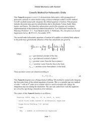
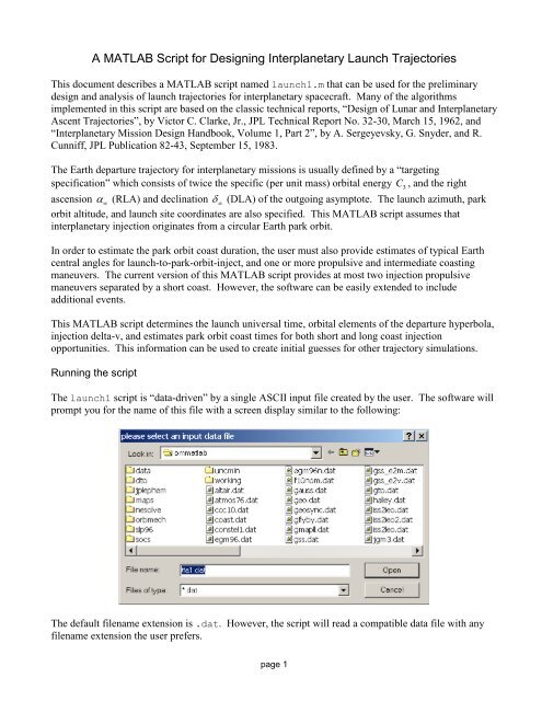
A MATLAB Script for Designing Interplanetary Launch TrajectoriesThis document describes a MATLAB script named launch1.m that can be used for the preliminarydesign and analysis of launch trajectories for interplanetary spacecraft. Many of the algorithmsimplemented in this script are based on the classic technical reports, “Design of Lunar and InterplanetaryAscent Trajectories”, by Victor C. Clarke, Jr., JPL Technical Report No. 32-30, March 15, 1962, and“Interplanetary Mission Design Handbook, Volume 1, Part 2”, by A. Sergeyevsky, G. Snyder, and R.Cunniff, JPL Publication 82-43, September 15, 1983.The Earth departure trajectory for interplanetary missions is usually defined by a “targetingspecification” which consists of twice the specific (per unit mass) orbital energy C3, and the rightascension (RLA) and declination (DLA) of the outgoing asymptote. The launch azimuth, parkorbit altitude, and launch site coordinates are also specified. This MATLAB script assumes thatinterplanetary injection originates from a circular Earth park orbit.In order to estimate the park orbit coast duration, the user must also provide estimates of typical Earthcentral angles for launch-to-park-orbit-inject, and one or more propulsive and intermediate coastingmaneuvers. The current version of this MATLAB script provides at most two injection propulsivemaneuvers separated by a short coast. However, the software can be easily extended to includeadditional events.This MATLAB script determines the launch universal time, orbital elements of the departure hyperbola,injection delta-v, and estimates park orbit coast times for both short and long coast injectionopportunities. This information can be used to create initial guesses for other trajectory simulations.Running the scriptThe launch1 script is “data-driven” by a single ASCII input file created by the user. The software willprompt you for the name of this file with a screen display similar to the following:The default filename extension is .dat. However, the script will read a compatible data file with anyfilename extension the user prefers.page 1

Input data filesThis section describes a typical input data file for the software. In the following discussion the actualinput file contents are in courier font and all explanations are in times italic font. The following is aninput data file for the Mars Exploration Rover mission. The information for this file was extracted from“Mission Design Overview for the Mars Exploration Rover Mission”, by Ralph B. Roncoli and Jan M.Ludwinski, AIAA 2002-4823.Each data item within a launch1 input file is preceded by one or more lines of annotation text. Do notdelete any of these annotation lines or increase or decrease the number of lines reserved for eachcomment. However, you may change them to reflect your own explanation. The annotation line alsoincludes the correct units and when appropriate, the valid range of the input. ASCII text input is notcase sensitive but must be spelled correctly.The first four lines of any input file are reserved for user comments. These lines are ignored by thesoftware. However the input file must begin with four and only four initial text lines.**********************************interplanetary injection data fileMER-A mission – mer-a.dat**********************************The first input item is the name of the simulation. This helps with traceability and will be displayedwith the screen display of the solution.mission name------------MER-A MissionThe next input is the launch calendar date of the simulation. Please include all 4 digits of thecalendar year.launch calendar date (month, day, year)5,30,2003The next data item is the launch azimuth in degrees.launch azimuth (degrees)93The next data item is the geodetic latitude of the launch site in degrees.launch site geodetic latitude (degrees)28.285579The next data item is the east longitude of the launch site in degrees.launch site east longitude (degrees)279.434701The next data item is the altitude of the circular park orbit.circular park orbit altitude (kilometers)185.2page 2

The next data item is the launch energy C3in the unit ofC3 (twice specific orbital energy; (km/sec)^2)9.282 2km sec .The next data item is the declination of the launch hyperbola, DLA, in degrees.DLA (declination of launch hyperbola; degrees)2.27The next data item is the right ascension of the launch hyperbola, RLA, in degrees.RLA (right ascension of launch hyperbola; degrees)352.59The next data item is an estimate of the Earth central angle from liftoff to park orbit injection, indegrees.central angle from launch to park orbit inject (degrees)24.0The next data item is an estimate of the Earth central angle of the first and perhaps onlyinterplanetary injection propulsive maneuver, in degrees.central angle for first injection maneuver (degrees)9.0The next data item is an estimate of the Earth central angle of a short coast between a first andsecond propulsive maneuver. If there is no second maneuver, set this value to 0.central angle between first and second injection maneuvers (degrees)7.0The next data item is an estimate of the Earth central angle for a second propulsive maneuver, indegrees. If there is no second maneuver, set this value to 0central angle for second injection maneuver (degrees)8.0The final data item is an estimate of the injection true anomaly on the departure hyperbola, indegrees. For an impulsive maneuver, this value is usually 0 which corresponds to perigee of thedeparture hyperbola. For a finite-burn maneuver, this value is non-zero and usually positive.injection true anomaly (degrees)8.0The injection true anomaly could also include an additional central angle increment that represents ashort coast to a target interface point (TIP) which is often part of a target specification. Some spacecraftmissions often require that C3, DLA and RLA be enforced at a TIP and not necessarily at burnout of theupper stage.page 3

Typical script simulation exampleThis section is a typical output provided by the launch1 MATLAB script. It illustrates thecharacteristics for both a short and long park orbit coast mission.-------------------------------------------------launch1.m - interplanetary launch characteristics-------------------------------------------------MER-A MissionOpportunity #1==============launch calendar date30-May-2003launch universal time 18:29:39.192launch azimuthlaunch site geodetic latitudelaunch site geocentric declinationlaunch site east longitude93.000000 degrees28.446462 degrees28.285572 degrees279.434701 degreeslaunch hyperbola characteristics--------------------------------c3asymptote declinationasymptote right ascensionsemimajor axis9.280000 (km/sec)^22.270000 degrees352.590000 degrees-42952.633782 kilometerseccentricity 1.15280406inclinationargument of perigeeraanorbital periodfirst park orbit coast timefirst park orbit coast anglerange anglerasc of launch site at 0 hrrasc of launch site at launch28.431148 degrees214.608488 degrees348.391220 degrees88.195573 minutes19.367145 minutes79.053538 degrees269.217201 degrees166.529456 degrees84.702262 degreespage 4

arglat of launch site at launchgreenwich sidereal time at 0 hrasymptote true anomalyasymptote argument of latitudeascending node to launch siteascending node to asymptotelocal circular velocityinjection velocityinjection delta-v95.554950 degrees247.094755 degrees150.163663 degrees4.772151 degrees96.311041 degrees4.198780 degrees7793.033366 meters/second11434.279080 meters/second3641.245714 meters/secondopportunity #2==============launch calendar date30-May-2003launch universal time 07:05:07.054launch azimuthlaunch site geodetic latitudelaunch site geocentric declinationlaunch site east longitude93.000000 degrees28.446462 degrees28.285572 degrees279.434701 degreeslaunch hyperbola characteristics--------------------------------c3asymptote declinationasymptote right ascensionsemimajor axis9.280000 (km/sec)^22.270000 degrees352.590000 degrees-42952.633782 kilometerseccentricity 1.15280406inclinationargument of perigeeraanorbital periodfirst park orbit coast time28.431148 degrees25.064186 degrees176.788780 degrees88.195573 minutes61.126695 minutespage 5

first park orbit coast anglerange anglerasc of launch site at 0 hrrasc of launch site at launcharglat of launch site at launchgreenwich sidereal time at 0 hrasymptote true anomalyasymptote argument of latitudeascending node to launch siteascending node to asymptotelocal circular velocityinjection velocityinjection delta-v249.509236 degrees79.672900 degrees166.529456 degrees273.099821 degrees95.554950 degrees247.094755 degrees150.163663 degrees175.227849 degrees96.311041 degrees175.801220 degrees7793.033366 meters/second11434.279080 meters/second3641.245714 meters/secondIn the launch1 solution display screens,rasc = right ascensionarglat = argument of latitude = sum of argument of perigee and true anomalyraan = right ascension of the ascending nodeThe output shown for ascending node to launch site and ascending node to asymptoteare the angles measured from the ascending node along the equator to the launch site at the launch timeand launch hyperbola asymptote, respectively. Also, since the calculations assume an initial circularpark orbit, the true anomaly on the hyperbola at injection is identically zero (injection occurs at perigee)and the argument of latitude of the maneuver is equal to the argument of perigee.Technical discussionThis section is a brief summary of the geometry and orbital mechanics involved in the design andanalysis of interplanetary injection trajectories.The following diagram, extracted from “JPL Publication 82-43, Interplanetary Mission DesignHandbook”, illustrates the basic geometry of the interplanetary launch problem. In this figure, represents inertial right ascension measured relative to the Vernal Equinox, represents geocentricdeclination measured relative to the Earth’s equator, is the launch azimuth measured positiveclockwise from true north, is the right ascension of the ascending node (RAAN), and Lis thegeocentric latitude of the launch site. Items with an “infinity” subscript refer to the hyperbolicasymptote of the outgoing or departure trajectory.Lpage 6

Departure trajectory orientationThe transfer trajectory must contain the launch site, the outgoing asymptote of the departure hyperbolaand the center of the Earth at the moment of launch. The constraining equation for this orientation ishs ˆ ˆ hˆ s ˆ hˆ s ˆ hˆs ˆ 0x x y y z zwhere ĥ is the unit angular momentum of the launch hyperbola and ŝ is a unit vector in the direction ofthe outgoing asymptote. This constraint forces the angular momentum vector of the departure trajectoryto be perpendicular to the outgoing asymptote.The departure asymptote unit vector given bycoscoss ˆ cossin sin where right ascension of departure asymptotedeclination of departure asymptoteFurthermore, the angular momentum unit vector must also satisfy the following dot product constraintˆ ˆ ˆˆ ˆ 2 2 2 h 1x hy hzhhpage 7

These two equations can be solved simultaneously to yield the following two equations for the x and ycomponents of the unit angular momentum vector.hˆxhˆsˆ hˆsˆy y z zsˆxhˆyhˆsˆ sˆ sˆ 1 sˆ hˆ2 2z y z x z z2 2sˆˆx syThe positive and negative sign in front of the square root in the second equation indicates that there aretwo possible launch time solutions. One solution corresponds to a short transfer and the other representsa long transfer mission.The z-component of the unit angular momentum vector can be determined from the orbital inclination ior the flight azimuth Land launch site geocentric declination Laccording tohˆ cosi cossin z L LNotice that it is physically impossible to have an orbit in whichh1s2 2z zIf the declination of the launch hyperbola is greater than the launch site latitude, there is a range ofazimuths (symmetric about east) at which launching is not possible.Therefore, launch azimuth is restricted such that the following constraint must be satisfied22 cos sin L2cos LFurthermore, the launch azimuth sector is symmetric about east with the following lower and upperlimits22 cos sin L LIMIT 2cos Launch timeWhen the launch site passes through the departure trajectory plane, the following two geometricconditions must be satisfiedrˆ h ˆ rˆ hˆ rˆ hˆ rˆ hˆ 0L Lx x Ly y Lzz2 2h ˆ r ˆ ˆ cos cos ˆLiz L hzLpage 8

where r ˆLis the inertial unit position vector of the launch site andˆzi is a unit vector aligned with theˆ i 0,0,1 T.Earth’s spin axis and is given by z The inertial unit position vector of the launch site can be determined fromcosLcosL r ˆL cosL sinL sinL where Lis the local sidereal time of the launch site at the time of launch t L. The local sidereal time atthe launch time can be determined from the following expressionwhere tEL g0L e Lg0ELGreenwich sidereal time at 0 hours UTeast longitude of launch site einertial rotation rate of the EarthThe local sidereal time is identical to the right ascension of a ground site.The previous two constraint equations can be solved simultaneously to yield the following equations forthe right ascension of the launch site at the launch timehˆ hˆ sinhˆ cos hˆsinLhˆ1 cos2 2y z L x L zhˆ hˆ sinhˆ cos hˆcosLhˆ1 cos2z2 2z x L y L z2zThese two equations should be evaluated with a four quadrant inverse tangent function to determine theright ascension of the launch site. The right ascension of the launch site as a function of launch azimuthis given by these next two equationshˆsinLhˆcosLsinsin hˆcos y L L x Lˆ2hz1sinsin hˆcos x L L y Lˆ2hz1LLpage 9

The three components of the unit angular momentum vector are functions of the launch azimuth and thecomponents of the outgoing asymptote unit vector. Therefore, for a given geographic launch site, thelaunch time is determined by the launch azimuth and the declination and right ascension of the outgoingasymptote.The right ascension of the launch site at the launch time is also given by tEL g0L e LFinally, this equation can be solved for the launch time to yieldtL EL g0LeLaunch azimuthFor a given launch site, launch time and outgoing asymptote, the corresponding flight azimuth can becomputed from the following two equationscosisin Lcoscos sin i cos LLLand the four quadrant inverse tangent tan sin ,cos 1 L L Lwhere is the right ascension of the descending node which can be determined from the followingexpression tan nˆ, nˆ1 y xIn this equation, ˆn is a unit vector pointing in the direction of the descending node. This vector can becomputed from the following cross productnˆhˆˆiwhere ˆzi is a unit vector aligned with the Earth’s spin axis and is given by ˆ Range angle and park orbit coast time estimatezi 0,0,1 T.The range angle is measured in the orbit plane from the launch site to the outgoing asymptote and can bedetermined fromz page 10

and the four quadrant inverse tangentsin Lcossinsin Lcos sin sin cos cos cos L L L tan 1sin ,cos The range angle is also equal to the following combination of Earth central angles and true anomalieswhere1N i2i c I1 launch-to-park orbit inject Earth central angle iEarth central angle for ic park orbit coast Earth central angle true anomaly of outgoing asymptote true anomaly at interplanetary injectionIthpropulsive or coast maneuverand N is the total number of additional propulsive or coasting maneuvers. The Earth central angle is thegeocentric angle measured along the orbit plane from the beginning to the end of an orbital event such asa coast or maneuver.The cosine of the range angle is also equal to the dot product of the unit inertial position vector of thelaunch site and the unit outgoing asymptote vector which is defined in the next section. Please seeAppendix B for additional information and a MATLAB function that computes the range angle usingthis approach.The park orbit coast Earth central angle is computed from Nc 1 i Ii21The true anomaly of the outgoing asymptote is given by cos 1 eof the departure trajectory is located relative to the outgoing asymptote. and determines where perigeeFinally, the coast time can be estimated from t c cn, where n is the two-body or Keplerian(unperturbed) mean motion of the park orbit and is equal tothe initial circular Earth park orbit.3 r poand rpois the geocentric radius ofpage 11

Departure hyperbola orbital characteristicsThis section describes the algorithm used to determine the Earth-centered-inertial (ECI) state vector of adeparture hyperbola for interplanetary missions. In the discussion that follows, interplanetary injectionis assumed to occur impulsively at perigee of the geocentric departure hyperbola. The method describedhere is based on the fundamental characteristics of the B-plane coordinate system.The departure trajectory for interplanetary missions is specified by the orbital energy C3, and the rightascension and declination of the outgoing asymptote. The perigee radius of the departurehyperbola is specified and the orbital inclination is computed from the user-defined launch azimuthand launch site geocentric latitude Lfrom the equationi cos cos Lsin L1 The algorithm used to design the departure hyperbola only works for geocentric orbit inclinations thatsatisfy the following constrainti A unit vector in the direction of the departure asymptote is given by coscosˆ S cossin sin Lwhere right ascension of departure asymptotedeclination of departure asymptoteThe T-axis direction of the B-plane coordinate system is determined from the following vector crossproduct:TˆSˆuwhere ˆ u 0 01 Tis a unit vector perpendicular to the Earth’s equator.z The following cross product operation completes the B-plane coordinate system.ˆ zRˆSˆTˆThe B-plane angle is determined from the orbital inclination of the departure hyperbola i and thedeclination of the outgoing asymptote according tocosicoscospage 12

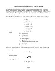
The unit angular momentum vector of the departure hyperbola is given byhˆ Tˆ sinRˆ cosThe sine and cosine of the true anomaly at infinity are given by the next two equationscosrV 22sin 1cospwhere V C 3V LV is the spacecraft’s velocity at infinity, pVLis the heliocentric departure velocitydetermined from the Lambert solution, Vpis the heliocentric velocity of the departure planet, and rpisthe user-specified perigee radius of the departure hyperbola.A unit vector in the direction of perigee of the departure hyperbola is determined fromrˆ ˆcos ˆ ˆp S h SsinThe ECI position vector at perigee isr r r ˆ .p p pThe scalar magnitude of the perigee velocity can be determined fromVp2 Vrp2A unit vector aligned with the velocity vector at perigee is v hˆ r ˆ . The ECI velocity vector atperigee of the departure hyperbola is given byv V v ˆ .p p pFinally, the classical orbital elements of the departure hyperbola can be determined from the positionand velocity vectors at perigee. The injection delta-v vector and magnitude can be determined from thevelocity difference between the park orbit and departure hyperbola at the orbital location of theimpulsive maneuver.An alternative algorithm for computing launch timeThis section describes a slightly different algorithm for computing launch time. It is based on informalnotes provided by Johnny Kwok at JPL.The equations for computing the classical orbital elements of the departure hyperbola are as follows:ˆ ppsemimajor axisaC 3page 13

orbital eccentricityr poe 1aorbital inclinationargument of perigeei cos cos Lsin L1 c for injection during the decending part of the park orbit1 sinL c sin sinifor injection during the ascending part of the park orbitright ascension of the ascending node1 sinL c 180 sin sini hwhere h is the angle from the ascending node to the launch asymptote projection on the equator,measured along the equator and determined from h tan c i c 1sin sin ,cos The launch time can be determined from this next set of calculations:The launch site sidereal time at 0 hours UTC (Universal Coordinated Time) is computed using .0 g0ELThe launch site local sidereal time at launch is given by L h g where g is the angle from theascending node to the launch site, measured along the equator and determined fromg tan sin d cos i,cos d L 1 For a launch azimuth L 90, the argument of latitude of the launch site d is given byd sin sini1 0 sin page 14

Otherwised1 sin0180 sin sini .Finally, the launch time can be determined fromtLL0eThe following diagram, also extracted from “JPL Publication 82-43, Interplanetary Mission DesignHandbook”, illustrates the important angular quantities and relative geometry involved in theinterplanetary launch problem. Please note that all angles are measured in the Earth’s equatorial plane.In this diagram, GMT should be replaced with the modern day definition, UTC.Geocentric Declination of the Launch SiteThis MATLAB script uses the following equation to calculate the geocentric declination of the launchsite given the geodetic latitude Land geodetic altitude h. sin 2L sin 2L1 1 L L f sin 4ˆ 2 2Lfh 1 2hˆ1 4hˆ1 4hˆ 1 In this equation, the geocentric distance r and geodetic altitude h have been normalized by ˆ r/ r eqandhˆ h r/ eq, respectively. reqis the equatorial radius of the Earth and f is the flattening factor.2page 15

Spherical EquationsThis section provides additional equations that may be useful for interplanetary mission design andanalysis. For example, they can be used to determine the characteristics of a launch hyperbola from theclassical orbital elements at the target interface point (TIP).The asymptote unit vector in terms of the classical orbital elements of a hyperbolic orbit is given by sin sinicoscos sin sin cosis ˆ sin cos cossin cosiIn this expression, is the right ascension of the ascending node (RAAN), is the argument ofperiapsis and is the true anomaly.The declination of the asymptote (DLA) is given by 1 1 sin sin sini sin sin usin iwhere u is the argument of latitude of the launch asymptote. In this expression is the trueanomaly of the launch hyperbola “at infinity” and is a function of the orbital eccentricity e of the1hyperbola according to cos 1 e.Finally, from the following two expressionstansin tanicosucos costhe right ascension of the asymptote (RLA) can be determined from1 tancosu tan , tanicos where the inverse tangent in this equation is a four quadrant operation.page 16

Algorithm resources(1) “Design of Lunar and Interplanetary Ascent Trajectories”, Victor C. Clarke, Jr., JPL TechnicalReport No. 32-30, March 15, 1962.(2) An Introduction to the Mathematics and Methods of Astrodynamics, Richard H. Battin, AIAAEducation Series, 1987.(3) Analytical Mechanics of Space Systems, Hanspeter Schaub and John L. Junkins, AIAA EducationSeries, 2003.(4) Spacecraft Mission Design, Charles D. Brown, AIAA Education Series, 1992.(5) Orbital Mechanics, Vladimir A. Chobotov, AIAA Education Series, 2002.(6) “A Computer Simulation of the Orbital Launch Window Problem”, Archie C. Young and Pat R.Odom, AIAA 67-615, 1967.(7) “Launch Parameters for Interplanetary Flights”, W. C. Riddell, American Rocket Society Journal,December 1960.(8) “Interplanetary Mission Design Handbook, Volume 1, Part 2”, JPL Publication 82-43, September 15,1983.(9) “Launch-on-Time Analysis for Space Missions”, JPL Technical Report No. 32-29, August 15, 1960.page 17

Appendix AGreenwich Apparent Sidereal TimeThis appendix describes the algorithm used in this MATLAB script to calculate Greenwich apparentsidereal time. This numerical method calculates the apparent Greenwich sidereal time using the firstfew terms of the IAU 1980 nutation algorithm.The Greenwich apparent sidereal time is given by the expressionwhere mis the Greenwich mean sidereal time,obliquity of the ecliptic and cos is the nutation in obliquity.The Greenwich mean sidereal time is calculated using the expressionmm is the nutation in longitude, mis the mean 2 3m 280.46061837 360.98564736629 JD 2451545.0 0.000387933 T T /38710000where T ( JD 2451545)/36525 and JD is the Julian date. The mean obliquity of the ecliptic isdetermined from0 2 3m 23 2621. 448 46. 8150T 0. 00059T 0. 001813TThe nutation in obliquity and longitude involves the following three trigonometric arguments (indegrees)L280.4665 36000.7698TL 218.3165 481267.8813T 125.04452 1934.136261TThe calculation of nutation uses the following two equationsThese corrections are in units of arc seconds. 17.20sin 1.32sin 2L 0.23sin 2L 0.21sin 2 9.20cos 0.57cos2L 0.10cos2L 0.09cos2The following is the MATLAB source code for this function.function gst = gast1 (jdate)% Greenwich apparent sidereal time% major nutation terms only% inputpage 18

% jdate = Julian date% output% gst = Greenwich apparent sidereal time (radians)% (0

Appendix BRange Angle CalculationThis appendix describes a technique for computing the range angle using unit vectors. The two unitvectors are assumed to be coplanar.The cosine of the transfer or “included” angle between two coplanar unit vectors measured relative tothe same celestial body is given bycos uˆu ˆThe sine of the transfer angle is given by1 2k ˆ 0 0 1 T.where 2uˆuˆ k ˆsin sign 1cos 1 2Finally, the transfer angle is calculated using the following expression tan sin ,coswhere the inverse tangent is a four quadrant calculation.1 The following is the MATLAB source code for this function.function rangle = range_angle(uhat1, uhat2)% range angle between two coplanar unit vectors% input% uhat1 = first unit vector% uhat2 = second unit vector% output% rangle = included angle between first and second unit vectors (radians)% NOTE: direction is from uhat1 to uhat2% Orbital Mechanics with Matlab%%%%%%%%%%%%%%%%%%%%%%%%%%%%%%%% unit "normal" vectorxkhat(1) = 0.0;xkhat(2) = 0.0;xkhat(3) = 1.0;page 20

% cosine of range anglectangle = dot(uhat1, uhat2);r1xr2 = cross(uhat1, uhat2);vdotwrk = dot(r1xr2, xkhat);% sine of range anglestangle = sign(vdotwrk) * sqrt(1.0 - ctangle^2);% range angle (radians)rangle = atan3(stangle, ctangle);page 21