Lectures on the Qualitative Theory Curves and Surfaces of ... - Unesp

PrefaceThese Lecture Notes are addressed to the reader with some familiarity with the Foundations ofOrdinary Differential Equations and Differential Geometry.The subject centers around the local geometry on a surface: Fundamental Forms, principalcurvatures, Gauss and Codazzi equations, Gauss–Bonnet Theorem. To represent a level, [9], [17],[20], [48], [50], [56], [74] and [75] can be mentioned.The authors believe that from the Introduction provided in these Lecture Notes, the reader maygo to consult the papers quoted here, where more complete treatments and details are presented,and become interested in some of the many lines of advanced study and research open in the fieldof interaction between Geometry and Analysis, outlined here.The scope of these Lecture Notes is to illustrate the penetration of ideas such as genericity andstructural stability of O.D.E’s in the development of the differential equations of classical geometry.These Lecture Notes are part of a more general work in current development.The authors are fellows of CNPq and done this work under the project CNPq 473747/2006-5.Ronaldo GarciaJorge SotomayorGoiânia, September 20083

ContentsPreface 31 Diff. Eq. of Classical Geometry 9Introduction 91.1 The First Fundamental Form . . . . . . . . . . . . . . . . . . . . . . . . . . . . . . . . . . . . 91.2 The Second Fundamental Form . . . . . . . . . . . . . . . . . . . . . . . . . . . . . . . . . . 101.3 Fundamental Equations . . . . . . . . . . . . . . . . . . . . . . . . . . . . . . . . . . . . . . . 111.4 Diff. Eq. of Curvature Lines . . . . . . . . . . . . . . . . . . . . . . . . . . . . . . . . . . . . . 121.5 Differential Equations of Asymptotic Lines . . . . . . . . . . . . . . . . . . . . . . . . . . . . 131.6 Differential Equations of Geodesics . . . . . . . . . . . . . . . . . . . . . . . . . . . . . . . . 141.7 Exercises . . . . . . . . . . . . . . . . . . . . . . . . . . . . . . . . . . . . . . . . . . . . . . . 152 Classical Results on Curvature Lines 17Introduction 172.1 Triple orthogonal systems . . . . . . . . . . . . . . . . . . . . . . . . . . . . . . . . . . . . . . 172.1.1 Ellipsoid with three different axes . . . . . . . . . . . . . . . . . . . . . . . . . . . . . 202.2 Envelopes of Regular Surfaces . . . . . . . . . . . . . . . . . . . . . . . . . . . . . . . . . . . 212.3 Examples of Umbilics on Algebraic Surfaces . . . . . . . . . . . . . . . . . . . . . . . . . . . 232.4 Exercises . . . . . . . . . . . . . . . . . . . . . . . . . . . . . . . . . . . . . . . . . . . . . . . 253 Global Principal Stability 27Introduction 273.1 Lines of curvature near Darbouxian umbilics . . . . . . . . . . . . . . . . . . . . . . . . . . . 273.1.1 Preliminaries concerning umbilic points . . . . . . . . . . . . . . . . . . . . . . . . . . 273.2 Hyperbolic Principal Cycles . . . . . . . . . . . . . . . . . . . . . . . . . . . . . . . . . . . . 313.3 A Theorem on Principal Stability . . . . . . . . . . . . . . . . . . . . . . . . . . . . . . . . . 333.4 Concluding Remarks . . . . . . . . . . . . . . . . . . . . . . . . . . . . . . . . . . . . . . . . . 333.5 Exercises . . . . . . . . . . . . . . . . . . . . . . . . . . . . . . . . . . . . . . . . . . . . . . . 344 Bifurcations of Umbilics 37Introduction 374.1 Umbilic Points of Codimension One . . . . . . . . . . . . . . . . . . . . . . . . . . . . . . . . 374.1.1 The D2,3 1 Umbilic Bifurcation Pattern . . . . . . . . . . . . . . . . . . . . . . . . . . . 404.2 Exercises . . . . . . . . . . . . . . . . . . . . . . . . . . . . . . . . . . . . . . . . . . . . . . . 435

6 CONTENTS5 Stability of Asymptotic Lines 45Introduction 455.1 Parabolic Points . . . . . . . . . . . . . . . . . . . . . . . . . . . . . . . . . . . . . . . . . . . 455.1.1 Computation of the Second Fundamental Form . . . . . . . . . . . . . . . . . . . . . 465.2 Stability of parabolic points . . . . . . . . . . . . . . . . . . . . . . . . . . . . . . . . . . . . . 505.3 Stability of Periodic Lines . . . . . . . . . . . . . . . . . . . . . . . . . . . . . . . . . . . . . . 505.3.1 Regular Periodic Asymptotic Lines. . . . . . . . . . . . . . . . . . . . . . . . . . . . . 505.3.2 Folded periodic asymptotic lines . . . . . . . . . . . . . . . . . . . . . . . . . . . . . . 525.4 Examples of Periodic Asymptotic Lines . . . . . . . . . . . . . . . . . . . . . . . . . . . . . . 545.4.1 A Hyperbolic periodic asymptotic line . . . . . . . . . . . . . . . . . . . . . . . . . . . 545.4.2 Semihyperbolic periodic asymptotic line . . . . . . . . . . . . . . . . . . . . . . . . . . 545.5 On a class of dense asymptotic lines . . . . . . . . . . . . . . . . . . . . . . . . . . . . . . . . 565.6 Further developments on asymptotic lines . . . . . . . . . . . . . . . . . . . . . . . . . . . . . 575.7 Exercises . . . . . . . . . . . . . . . . . . . . . . . . . . . . . . . . . . . . . . . . . . . . . . . 586 Closed Geodesics 61Introduction 616.0.1 Closed Geodesics . . . . . . . . . . . . . . . . . . . . . . . . . . . . . . . . . . . . . . 616.0.2 Geodesics on Surfaces of Revolution . . . . . . . . . . . . . . . . . . . . . . . . . . . . 636.0.3 Remarks on the Geodesic Flow on a Sphere . . . . . . . . . . . . . . . . . . . . . . . . 646.1 Exercises . . . . . . . . . . . . . . . . . . . . . . . . . . . . . . . . . . . . . . . . . . . . . . . 65Bibliography 66

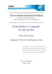
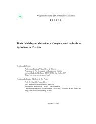
List of Figures2.1 Triple orthogonal system of quadratic surfaces . . . . . . . . . . . . . . . . . . . . . 202.2 Curvature lines of the Ellipsoid . . . . . . . . . . . . . . . . . . . . . . . . . . . . . . 212.3 Canal surface with variable radius . . . . . . . . . . . . . . . . . . . . . . . . . . . . 223.1 Darbouxian Umbilic Points, corresponding L α surface and lifted line fields. . . . . . 303.2 Lines of Curvature near Darbouxian Umbilic Points . . . . . . . . . . . . . . . . . . 314.1 Umbilic Point D2 1 and bifurcation . . . . . . . . . . . . . . . . . . . . . . . . . . . . 394.2 Lie-Cartan suspension D2,3 1 . . . . . . . . . . . . . . . . . . . . . . . . . . . . . . . . 414.3 Umbilic Point D2,3 1 and bifurcation. . . . . . . . . . . . . . . . . . . . . . . . . . . . . 435.1 Asymptotic lines near a parabolic line . . . . . . . . . . . . . . . . . . . . . . . . . . 485.2 Folded periodic asymptotic lines . . . . . . . . . . . . . . . . . . . . . . . . . . . . . 535.3 Asymptotic lines on the torus . . . . . . . . . . . . . . . . . . . . . . . . . . . . . . . 566.1 Geodesics on the surfaces of revolution . . . . . . . . . . . . . . . . . . . . . . . . . 647

8 LIST OF FIGURES

Chapter 1Differential Equations of ClassicalGeometryIntroductionIn this chapter the basic notions of differential geometry of curves and surfaces in R 3 will bereviewed. The differential equations of geodesics, principal curvature lines and asymptotic lines willbe obtained.The references for this chapter are [3], [9], [16], [17], [20], [42], [74] and [75].The principal curvature lines are the integral curves along the directions which the surfacebends extremely. It can be said that the theory of curvature lines was founded by G. Monge(1796), who determined explicitly the principal curvature lines of the ellipsoid with different axes.This is probably the first example in the literature of singular foliations.The geodesics is also a classical notion and are obtained as a critical points (local minimizers ofthe length) via the Calculus of Variations. They can be regarded, infinitesimally, as the curves ofzero geodesic curvature.The asymptotic lines are characterized geometrically as the curves where the osculating planecoincides with the tangent plane of the surface.1.1 The First Fundamental FormLet α : M 2 → R 3 be a C r , r ≥ 4, immersion of an oriented smooth surface M into R 3 .This space is oriented by a once for all fixed orientation and is endowed with the Euclideaninner product 〈, 〉. Let N be the vector field orthonormal to α defining the positive orientation ofM. This means that if (u,v) is a positive chart then {α u ,α v ,N} is a positive frame in R 3 .The induced metric on T p M is defined by 〈u,v〉 p:= 〈Dα(p)u, Dα(p)v〉, where u, v ∈ T p M.In a local chart (u,v) : M → R 2 , consider a parametric curve c(t) = (u(t),v(t)). Then it followsthat x(t) = (α ◦ c)(t) is a curve and x ′ = α u u ′ + α v v ′ is a tangent vector of T p M, where p = c(0).Therefore, 〈x ′ ,x ′ 〉 = 〈α u ,α u 〉 (u ′ ) 2 + 2 〈α u ,α v 〉u ′ v ′ + 〈α v ,α v 〉 (v ′ ) 2 and the expressionds 2 = Edu 2 + 2Fdudv + Gdv 2 (1.1)9

10 CHAPTER 1. DIFF. EQ. OF CLASSICAL GEOMETRYwhere E = 〈α u ,α u 〉, F = 〈α u ,α v 〉 and 〈α v ,α v 〉, is called the first fundamental form of α. Thisform is positive definite, i.e., E > 0, G > 0 and EG − F 2 > 0.by:The distance, in the induced metric, between two points c(t 0 ) and c(t 1 ) on the curve c is defineds =∫ t1t 0√E( dudt )2 + 2F( dudt )(dv dt ) + G(dv dt )2 dtA change of coordinates u = u(x,y) and v = v(x,y) gives du = u x dx + u y dy and dv =v x dx + v y dy.Therefore,Edu 2 + 2Fdudv + Gdv 2 =E(u x dx + u y dy) 2 + 2F(u x dx + u y dy)(v x dx + v y dy) + G(v x dx + v y dy) 2=[E(u x ) 2 + 2Fu x v x + G(v x ) 2 ]dx 2 + 2[Eu x u y + F(u x v y + u y v x ) + Gv x v y ]dxdy (1.2)+[E(u y ) 2 + 2Fu y v y + G(v y ) 2 ]dy 2=Ēdx2 + 2 ¯Fdxdy + Ḡdy2The angle between two directions, defined in a local chart by, dx = α u du + α v dv and dy =α u δu + α v δv is defined by:cos θ = 〈dx,dy〉|dx||dy|Therefore the angle between the parametric curves u = constant and v = constant is given by:Fcos θ = √EGand sin θ =√EG−F 2√EG.1.2 The Second Fundamental FormThe second fundamental form is introduced in order to define the concept of curvature of asurface. Let x(s) = α(u(s),v(s)) be the spatial curve and suppose that |x ′ | = 1, i.e. , x isparametrized by arc length. The curvature vector k(s) = dTdxdswhere T(s) =dshas the orthogonaldecomposition k = k n N + k g N ∧ T and k n is called the normal curvature and k g is called thegeodesic curvature.From 〈T,N〉 = 0 it follows that 〈 dTds ,N〉 = − 〈 T, dN 〉ds and therefore kn = − 〈dα,dN〉〈dα,dα〉 .So it is obtainedk n = edu2 + 2fdudv + gdv 2Edu 2 + 2Fdudv + Gdv 2 .Here, e = − 〈α u ,N u 〉, 2f = −(〈α u ,N v 〉 + 〈a v ,N u 〉) and g = − 〈α v ,N v 〉.Also, as 〈α u ,N〉 = 〈α v ,N〉 = 0 it follows thate = 〈α uu ,N〉 , f = 〈α uv ,N〉, g = 〈α vv ,N〉 .Using the expression of N = αu∧αv|α u∧α v|it is obtained thate = [α u,α v ,α uu ]√EG − F2 , f = [α u,α v ,α uv ]√EG − F2 , g = [α u,α v ,α vv ]√EG − F2 ,where [.,.,.] means the mixed product of three vectors in R 3 .

1.3. FUNDAMENTAL EQUATIONS 11The quadratic formis called the second fundamental form of α.II α = edu 2 + 2fdudv + gdv 2A change of coordinates u = u(x,y) and v = v(x,y) givesdu = u x dx + u y dy and dv = v x dx + v y dy.Thereforeedu 2 + 2fdudv + gdv 2 =e(u x dx + u y dy) 2 + 2f(u x dx + u y dy)(v x dx + v y dy) + g(v x dx + v y dy) 2= [e(u x ) 2 + 2fu x v x + g(v x ) 2 ]dx 2 + 2[eu x u y + f(u x v y + u y v x ) + gv x v y ]dxdy (1.3)+ [e(u y ) 2 + 2fu y v y + g(v y ) 2 ]dy 2= ēdx 2 + 2 ¯fdxdy + ḡdy 2The geodesic curvature k g is defined by the equationk g = 〈 (N ∧ T),T ′〉 = [T,T ′ ,N].The unit vector T satisfies the equation T = α u u ′ + α v v ′ , henceTherefore, the expression for k g is as follows:T ′ = α uu (u ′ ) 2 + 2α uv u ′ v ′ + α vv (v ′ ) 2 + u ′′ α u + v ′′ α v[Γ 2 11(u ′ ) 3 + (2Γ 2 12 − Γ 1 11)(u ′ ) 2 v ′ + (Γ 2 22 − 2Γ 1 12)u ′ (v ′ ) 2 − Γ 1 22(v ′ ) 3 + u ′ v ′′ − u ′′ v ′ ]√EG − F2For the parametric curves it follows that:√ √EG − F(k g ) v=c = Γ 2 2EG − F11E √ E , (k g) u=c = −Γ 1 222G √ G .In particular when the parametric curves are orthogonal (F = 0) it is obtained that:(k g )| v=v0 = − E v2E √ G = − dds 2ln √ E, (k g )| u=u0 =G u2G √ E = − dds 1ln √ G (1.4)The equation above shows that the geodesic curvature depends only of the first fundamental formand therefore is an intrinsic entity.1.3 Fundamental EquationsThe two fundamental forms, which define the length and curvature of curves on surfaces arerelated by the Fundamental Equations of Surface Theory.The first relation is obtained writing the vectors α uu , α uv , α vv , N u and N v in terms of theframe {α u ,α v ,N}.Direct calculation givesα uu = Γ 1 11 α u + Γ 2 11 α v + eNα uv = Γ 1 12 α u + Γ 2 12 α v + fNα vv = Γ 1 22 α u + Γ 2 22 α v + gN(1.5)(EG − F 2 )N v = (gF − fG)α u + (fF − gE)α v(EG − F 2 )N u = (fF − eG)α u + (eF − fE)α v

12 CHAPTER 1. DIFF. EQ. OF CLASSICAL GEOMETRYwhere the Christoffel symbols are given by:Γ 1 11Γ 1 12Γ 1 22= EuG−2FuF+EvF2(EG−F 2 )= EvG−GuF2(EG−F 2 )= 2FvG−GuG−GvF2(EG−F 2 )Γ 2 11 = 2FuE−EvE+EuF2(EG−F 2 )Γ 2 12 = GuE−EvF2(EG−F 2 )Γ 2 11 = GvE−2FvF+GuF2(EG−F 2 )(1.6)Differentiating the equations (α uu ) v = (α uv ) u and (α uv ) v = (α vv ) u the following equations ofcompatibility are obtained.−E eg−f2 = ∂Γ2 EG−F 2 12∂u − ∂Γ2 11∂v + Γ1 12 Γ2 11 − Γ1 11 Γ2 12 + Γ2 12 Γ2 12 − Γ2 11 Γ2 22−F eg−f2 = ∂Γ1 EG−F 2 12∂u − ∂Γ1 11∂v + Γ1 12 Γ2 12 − Γ2 11 Γ1 22∂e∂v − ∂fThese equations are called the Equations of Codazzi(1.7)∂u= eΓ 1 12 + f(Γ2 12 − Γ1 11 ) − gΓ2 11 ,∂f∂v − ∂g∂u= eΓ 1 22 + f(Γ2 22 − Γ1 12 ) − gΓ2 12 . (1.8)Remark 1.3.1. The method of moving frames developed by E. Cartan is also useful to present thestructure equations of Surface Theory. See [67].1.4 Differential Equations of Curvature LinesThe normal curvature in the direction [du : dv] also denoted by λ = dv/du is given by:k n = edu2 + 2fdudv + gdv 2 e + 2fλ + gλ2Edu 2 =+ 2Fdudv + Gdv2 E + 2Fλ + Gλ 2.The extremal values of k n are characterized by dkndλ = 0.Direct calculations, applying the Lagrange multipliers, it results that:k n = III = f + gλF + Gλ = e + fλE + FλTherefore the quadratic equation in λ is obtainedOr equivalently,(Fg − Gf)λ 2 + (Eg − Ge)λ + (Ef − Fe) = 0Fg − Gf)dv 2 + (Eg − Ge)dudv + (Ef − Fe)du 2 = 0 (1.9)⎛⎞dv 2 −dudv du 2⎜⎟det⎝E F G ⎠ = 0e f gAlso, the equation above can be interpreted as the annihilation of Jacobian of the map (du,dv) →(II(du,dv),I(du,dv)).∂(II,I)∂(du,dv)= 4(edu + fdv)(Fdu + Gdv) − 4(fdu + gdv)(Edu + Fdv) = 0

1.5. DIFFERENTIAL EQUATIONS OF ASYMPTOTIC LINES 13This equation defines two directions dvdu , in which k n attains the extremal values, minimal andmaximal. Its are called principal directions and the correspondent curvatures are called principalcurvatures.The normal curvature in the principal directions will be denoted by k 1 (minimal curvature) andk 2 (maximal curvature).The principal directions are well defined outside the points where the two fundamental formsare proportional, i. e. k 1 = k 2 . These points are called umbilic points and the set of umbilic pointswill be denoted by U α .Another geometrical interpretation of the differential equation of curvature lines is obtainedfrom the Rodrigues’ equationdN + kdp = 0, which defines the principal curvatures and theprincipal directions as eigenvalues and eigenvectors of the selfadjoint operator dN.Outside the umbilic set the principal directions are orthogonal and define two lines fields, calledprincipal lines fields which will be denoted by L 1 (α) and L 2 (α).In fact, it follows thatGλ 1 λ 2 + F(λ 1 + λ 2 )F + E= −1 [G(eF − fE) − F(eG − gE) − E(gF − Gf)] = 0gF − GfThe integral curves of these line fields are called principal curvature lines or simply principallines. The principal foliations formed by the principal lines will be denoted by P 1 (α) and P 2 (α).The triple P α = {P 1 (α), P 2 (α), U α } is called the principal configuration of the immersion α.The implicit differential equationH(u,v,[du : dv]) = (Fg − Gf)dv 2 + (Eg − Ge)dudv + (Ef − Fe)du 2 = 0defines in the projective bundle PM a surface H −1 (0). This surface in general is regular butcan present singularities.The line field in the chart (u,v,p), p = dvdu, defined by,∂X H = H p∂u + pH ∂p∂v − (H u + pH v ) ∂ ∂pis called a Lie-Cartan line field.In the chart (u,v,q), q = dudv, the line field is defined by,∂X H = qH q∂u + H ∂q∂v − (H v + qH u ) ∂ ∂q .The projections of the integral curves of X H by π(u,v,[du : dv]) = (u,v) are the principalcurvature lines.The projection π is a double covering outside the umbilic set U α and π −1 (p 0 ) = P 1 (R) at anumbilic point p 0 .1.5 Differential Equations of Asymptotic LinesThe normal curvature in a direction which makes an angle θ with a minimal principal directionis given, from Euler’s theorem, by:k n = k 1 cos 2 θ + k 2 sin 2 θ

14 CHAPTER 1. DIFF. EQ. OF CLASSICAL GEOMETRYThe directions where k n = 0 are called asymptotic directions and therefore are defined byII = edu 2 + 2fdudv + gdv 2 = 0.The line fields of asymptotic directions will be denoted by A 1 and A 2 . Its are called asymptoticline fields.It can be proved that the ordered pair {A 1 , A 2 } is well defined in the hyperbolic region of thesurface, where these directions are real.At the parabolic points defined by K = 0 the two asymptotic directions coincide and are welldefined when one principal curvature is not zero.The triple A α = {A 1 , A 2 , P α } is called the asymptotic configuration of the immersion α.The method of Lie-Cartan can be developed to consider the implicit differential equation ofasymptotic lines as a surface in the projective bundle PM.The asymptotic lines are the projections of the integral curves of Lie-Cartan line field. See [3].Proposition 1.5.1. Let α be in Imm k,k (M, R 3 ). Suppose that H α = {p : K(p) ≤ 0} is a regularsurface with boundary ∂H a = P α . Then the implicit surface of the asymptotic directions L(u,v,[du :dv] = edu 2 +2fdudv+gdv 2 = 0 is a regular surface in the projective bundle PM and the Lie-Cartanline field X L = L p∂∂u + pL p ∂ ∂v − (L u + pL v ) ∂ ∂p is globally defined in L−1 (0) and it is singular at thepoints where the asymptotic directions are tangent to the parabolic set P α .The asymptotic foliations of α are the integral foliations A 1α of l 1α and A 2α of l 2α ; they fill outthe hyperbolic region H α . When non-empty, the region H α is bounded by the set (generically, i.e.for most α ′ s, a regular curve [21], [47], [8], [10], P α of parabolic points of α, on which K α vanishes.On P α , the pair of asymptotic directions degenerate into a single one or into the whole tangentplane (at flat umbilic points, which generically are disjoint from the parabolic curve).1.6 Differential Equations of GeodesicsThe geodesics are the curves on the surface of zero geodesic curvature.Also the geodesics are defined as the curves of shortest distance between two points.The equation which defines the geodesic curvature k g of a curve parametrized by arc length sis given by the following expression:[Γ 2 11 (u′ ) 3 + (2Γ 2 12 − Γ1 11 )(u′ ) 2 v ′ + (Γ 2 22 − 2Γ1 12 )u′ (v ′ ) 2 − Γ 1 22 (v′ ) 3 + u ′ v ′′ − u ′′ v ′ ]√EG − F 2where u ′ = duds and v′ = dvds .Differentiating the equations 〈T ′ ,α u 〉 = 0 and 〈T ′ ,α v 〉 = 0 with respect to s the followingsystem is obtained.d 2 u+ Γ 1 ds 2 11 (du ds )2 + 2Γ 1 12 dudsd 2 v+ Γ 2 ds 2 11 (du ds )2 + 2Γ 2 12 dudsdvds + Γ1 22 (dvds )2 = 0dvds + Γ2 22 (dv ds )2 = 0Eliminating ds 2 = Edu 2 + 2Fdudv + Gdv 2 from the system above it follows that:(1.10)

1.7. EXERCISES 15d 2 vdu 2 = Γ1 22( dvdu )3 + (2Γ 1 12 − Γ 1 22)( dvdu )2 + (Γ 1 11 − 2Γ 2 12) dvdu − Γ2 11Or equivalently,d 2 udv 2 = Γ2 11( dudv )3 − (Γ 1 11 − 2Γ 2 12)( dudv )2 − (2Γ 1 12 − Γ 2 22) dudv − Γ1 22Proposition 1.6.1. Let M be a regular surface of class C k , k ≥ 2. Then for every p ∈ M andv ∈ T p M, v ≠ 0, there exist ǫ > 0 and an unique geodesic γ : (−ǫ,ǫ) → M such that γ(0) = p andγ ′ (0) = v.Proof. This follows from the theorem of existence and uniqueness for ordinary differential equationapplied to the vector field defined by:u ′ = 1v ′ = w(1.11)w ′ = Γ 1 22 w3 + (2Γ 1 12 − Γ1 22 )w2 + (Γ 1 11 − 2Γ2 12 )w − Γ2 111.7 Exercises1) Let p be a non umbilic point of S. Show that a neighborhood of p can be parametrized by principalcurvature lines. Write the Codazzi equations in a principal chart which is chacterized by f = F = 0.2) Let p be a hyperbolic point of S. Show that a neighborhood of p can be parametrized by asymptoticlines. Write the Codazzi equations in an asymptotic chart which is chacterized by e = g = 0.3) [ Bonnet coordinates on a convex surface ] Suppose M be a smooth surface in the euclidian spaceR 3 . Let p ∈ M such that K ≠ 0. and N : M → S 2 the normal Gauss map. Suppose an orthonormalreferential such that N(p) = (0, 0, −1).Let also π : S 2 \ {(0, 0, 1)} → R 2 be the stereographic projection.Consider the map β : U ⊂ R 2 → M defined by β = (π ◦ N) −1 .Introduce the support function f(u, v) = (1+u 2 + v 2 )D(u, v) where D is the distance (with signal) ofT β(u,v) M and the origin 0 ∈ R 3 . So it follows that β(u, v) = x(u, v), y(u, v), z(u, v)) is given by:x(u, v) = 1 2 f u − u uf u + vf v − fu 2 + v 2 + 1y(u, v) = 1 2 f v − v uf u + vf v − fu 2 + v 2 + 1z(u, v) = uf u + vf v − fu 2 + v 2 + 1(1.12)i) Show that in the coordinates of Bonnet above the differential equation of curvature lines is given by:f uv (du 2 − dv 2 ) + (f vv − f uu )dudv = 0 (1.13)ii) Let z = u+iv and ∂ ∂¯z = ∂∂u +i ∂∂vthe conjugate operator. Then show that equation (1.13) is equivalentto Im(f¯z¯z d¯z 2 ) = Im(f zz dz 2 ) = 0. See also [11].

16 CHAPTER 1. DIFF. EQ. OF CLASSICAL GEOMETRY4) Show that the differential equation of geodesics on an implicit surface F(x, y, z) = 0 is given by:F x F y F zdx dy dz= 0, F x dx + F y dy + F z dz = 0.∣d 2 x d 2 y d 2 z∣5) Show that the differential equation of principal curvature lines on an implicit surface F(x, y, z) = 0 isgiven by:∣ dx dy dz ∣∣∣∣∣∣ F x F y F z = 0, F x dx + F y dy + F z dz = 0.∣dF x dF y dF z6) Let (u, v) be a local positive principal chart on a surface S. Express the geodesic curvatures (seeequation (1.4)) of the coordinates lines in function of the principal curvatures k 1 and k 2 and theirderivatives, i.e., show thatk g | v=v0 (u, v 0 ) = −(k 2) uk 2 − k 1(u, v 0 ),k g | u=u0 (u 0 , v) = −(k 1) vk 2 − k 1(u, v 0 ),7) Given a parametric smooth surface α : U → R 3 define the square distance function D : U ×R 3 → R bythe equation D(u, v, p) = |p −α(u, v)| 2 . Geometrically D is a measure of contact between the surfacesand spheres in R 3 .In terms of singularities of D define the focal set of α and study its singularities. For a guide see [58].This subject is still a fecund source of current research.8) Show that the theory of principal curvature lines on surfaces of R 3 and that of the unitary sphereS 3 ⊂ R 4 is the same. More precisely, consider the stereographic projection π : S 3 \ {N} → R 3 .Write the expression of pi in coordinates and show that π is a conformal map. Conclude that π is aconjugaction between the principal configuration of the surface S ⊂ R 3 and that of ¯S = π −1 (S) ⊂ S 3 .See [51] for a geometric proof of the conformality of π.9) Show that an oriented connected surface having both principal curvatures constant, or, equivalently,those such that the Mean and Gauss curvatures are constant, is an open set of the plane, of a sphere,or of a circular right cylinder. See [66].10) Let S be a surface of revolution parametrized byα(s, v) = (r(s)cos v, r(s)sin v, z(s)).Consider a geodesic line γ(t) of S making an angle α(t) with the meridians and let r(t) the radiusof the correspondent parallel. Write the diffeential equation of the geodesic lines and show thatr(t)sin α(t) = cte.11) Let c be a closed principal line of a surface S. Show that a tubular neighoborhood of c can beparametrized such that the coordinates curves orthogonal to c are principal lines of S.

Chapter 2Classical Results on Curvature LinesIntroductionIn this chapter it will be considered triple orthogonal systems of surfaces in R 3 , envelope ofsurfaces and also some examples of umbilic points on algebraic surfaces.The basic references for this chapter are [16], [20], [44], [48], [50], [74], [75] and [79].For beautiful illustrations of sculptures of surfaces see [22] and [43].2.1 Triple orthogonal systemsTheorem 2.1.1 (Joachimsthal Theorem). Let two surfaces M 1 and M 2 intersecting along a curveγ on which their normals N 1 and N 2 make constant angle, i.e. 〈N 1 ,N 2 〉 |γ is constant, and suchthat DN 1 γ ′ ∧ γ ′ = 0. Then also it is verified that DN 2 γ ′ ∧ γ ′ = 0. In other words, if two surfacesintersect with constant angle along a curve which is the union of principal lines and umbilic pointsof the first one, this is also the case for the second one.Conversely, if DN 1 γ ′ ∧ γ ′ = 0 and DN 2 γ ′ ∧ γ ′ = 0 along a curve γ of intersection of M 1 andM 2 , then the angle between the surfaces, i.e., 〈N 1 ,N 2 〉 | γ is constant.Proof. By hypothesis the mixed product [N 1 ,N 2 ,γ ′ ] is not zero. So, differentiating the equation〈N 1 ,N 2 〉 = c it follows that [N 1 ,DN 2 (γ)γ ′ ,γ ′ ] = −[DN 1 (γ)γ ′ ,N 2 ,γ ′ ] = 0. This implies thatDN 2 (γ)γ ′ = λγ ′ . By Rodrigues formula it follows that γ is a cuvature line of M 2 . The reciprocalis direct. This ends the proof.From this follows directly that the principal configurations for surfaces of revolution are given bythe umbilic points which are at the poles and eventually on some parallels; the principal foliationsare given by arcs of non umbilical meridians and parallels.For a non spherical ellipsoid of revolution, however, the unique umbilic points occur at theirpoles, as follows from a direct calculation.Definition 2.1.2. A diffeomorphism preserving the orientation H : U ⊂ R 3 → R 3 , where U is anopen set and such that〈H u ,H v 〉 = 〈H u ,H w 〉 = 〈H v ,H w 〉 = 0, H u = ∂H∂u17

18 CHAPTER 2. CLASSICAL RESULTS ON CURVATURE LINESis called a triple orthogonal system..The simple examples of triple orthogonal systems are the cylindrical and spherical coordinatesin 3-space.In cylindrical coordinates, two families are formed of planes and the other consists of circularcylinders.In spherical coordinates, the first family is formed of concentric spheres with center at 0, thesecond is formed of planes containing one coordinate axis and the third is formed by cones.For each coordinate fixed, for example, w the map (u,v) → H w (u,v) = H(u,v,w) is aparametrization of a surface.Lemma 2.1.1. Let p = |H u |, q = |H v | and r = |H w | The following relations holds,H u ∧ H w = qrp H uH w ∧ H u = prq H v〈H u ,H vw 〉 = 0 〈H v ,H uw 〉 = 0 〈H w ,H uv 〉 = 0〈H u ,H v ∧ H w 〉 = pqrH u ∧ H v = pqr H w(2.1)Proof. Consider the unitary vector fields N 1 = H u /|H u |, N 2 = H v /|H v | and N 3 = H w /|H w |.By the hypothesis it follows that N 1 ∧N 2 = N 3 , N 2 ∧N 3 = N 1 , N 3 ∧N 1 = N 2 and 〈N 1 ,N 2 ∧ N 3 〉 =1. Then H u ∧ H v = pN 1 ∧ qN 2 = pqN 3 = pqr H w. The same for the other relations.Differentiating the equation 〈H u ,H v 〉 = 0 in relation to w it follows that 〈H uw ,H v 〉+〈H u ,H vw 〉 =0. Also it holds that 〈H uv ,H w 〉 + 〈H u ,H vw 〉 = 0 and 〈H uv ,H w 〉 + 〈H v ,H uw 〉 = 0.So, 〈H uw ,H v 〉 = − 〈H u ,H vw 〉 = −(− 〈H uv ,H w 〉) = − 〈H v ,H uw 〉. The same for the otherrelations. This ends the proof.Proposition 2.1.1. Consider the parametrized surfaces S 1 : (u,v) → H w (u,v) = H(u,v,w),S 2 : (w,u) → H v (w,u) = H(u,v,w) and S 3 : (v,w) → H u (v,w) = H(u,v,w).Then the coefficients of the first fundamental E i , F i and G i and of the second fundamental forme i , f i and g i of the surfaces S i , i = 1,2,3 are given by:I 1 = p 2 du 2 + q 2 dv 2I 2 = r 2 dw 2 + p 2 du 2I 3 = q 2 dv 2 + r 2 dw 2II 1 = − pp wr du2 − qq wr dv2II 2 = − rr vq dw2 − pp vq du2II 3 = − qq up dv2 − rr up dw2 (2.2)Proof. By the lemma 2.1.1 it follows that F i = f i = 0 for the three parametrized surfaces.The positive normal vector field to the surface S 1 is given by N 3 , for S 2 is N 2 and for S 3 is N 1 .Consider the surface S 2 : (w,u) → H v (w,u). Then it follows that〈 〉Hve 2 = 〈N 2 , H ww 〉 =|H v | , H ww〈 〉Hvg 2 = 〈N 2 , H uu 〉 =|H v | , H uuThe same for the other two surfaces.= − 〈H vw , H w 〉/|H v | = − |H w| 2 v2q= − 〈H uv , H u 〉/|H v | = − |H u| 2 v2q= − rr vq= − pp vq .

2.1. TRIPLE ORTHOGONAL SYSTEMS 19Remark 2.1.3. The local inverse G of the diffeomorphism H = (h 1 ,h 2 ,h 3 ) is called an orthogonalcoordinate system in the space. That is (for G i = ∂G∂c i),〈G i ,G j 〉 = 0, for i ≠ j (2.3)as follows from a direct calculation that gives G i = ∇h i /|∇h i | 2 .Theorem 2.1.4 (Dupin). The intersection of the level surface foliations M 2 (c 2 ) = {h 2 = c 2 } andM 3 (c 3 ) = {h 3 = c 3 } with a surface M 1 (a 1 ) = {h 1 = a 1 } produce on it a net of curves, along eachof which, say γ, holds that DN 1 γ ′ ∧ γ′ = 0; that is, γ is the union of principal curves and umbilicpoints of M 1 .Proof. Direct consequence of the proposition 2.1.1.Remark 2.1.5. Notice that it has been proved that the coordinate surfaces of any orthogonal coordinatesystem G in the space meet along common principal curves. A fact that is actually equivalentto the previous formulation of Dupin’s Theorem.Remark 2.1.6. By taking the ruled surfaces generated by the normal lines to a surface M alongprincipal lines, two families N 1v , based on minimal principal lines (say, v =constant), and N 2u ,based on maximal principal ones (say u = constant), are produced. These families of surfaces,together with the family M r given by parallel translation, are triply orthogonal. This shows that atnon umbilic points, any surface can be embedded in a family of surfaces which is part of a triplyorthogonal system.To prove that inversions I(p) = p/|p| 2 preserve lines of curvature, use the fact that these mapsare conformal (i.e. preserve angles). Apply Dupin’s Theorem to the image of the triple orthogonalsystem of surfaces just defined.Remark 2.1.7. A family of surfaces given by h(u,v,w) = c, may be part of a triple orthogonalsystem if the function h satisfy the differential equationSee [81].( ) ∂div∂n rot(n) = 0, n = ∇h|∇h| .Theorem 2.1.8 (Darboux). Suppose that two families of orthogonal surfaces intercept along linesof curvature. Then there exists a third family of surfaces orthogonal to the first two families.Proof. Consider two distribuitions ∆ 1 and ∆ 2 of tangent planes to the two families of orthogonalsurfaces. Define the distribuition ∆ 3 orthogonal to both ∆ 1 and ∆ 2 .Take unit vector fields X, Y such that X ∈ ∆ 1 ∩ ∆ 3 and Y ∈ ∆ 2 ∩ ∆ 3 .By hypothesis, as the intersection between the two families are curvature lines, it follows that∇ X Y = fX and ∇ Y X = gY . So, the Lie bracket [X,Y ] = ∇ X Y − ∇ Y X = fX − gY ∈ ∆ 3 .Therefore ∆ 3 is integrable and by Frobenius theorem, see [13] and [74], the third family of surfacesexists.

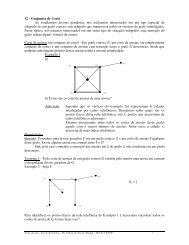
2.2. ENVELOPES OF REGULAR SURFACES 21M(u,v,w) = w 2 (u + w 2 )(v + w 2 ), W(a,b,c) = (a 2 − b 2 )(a 2 − c 2 ),u ∈ (−b 2 , −c 2 ) and v ∈ (−a 2 , −b 2 ).The first fundamental form of α is given by:I = ds 2 = Edu 2 + Gdv 2 = 1 4The second fundamental form of α is given by:II = edu 2 + gdv 2 =(u − v)udu 2 + 1 h(u) 4(v − u)vdv 2h(v)abc(u − v)4 √ abc(v − u)uvh(u) du2 +4 √ uvh(v) dv2 ,where h(x) = (x + a 2 )(x + b 2 )(x + c 2 ). The √ four umbilic √ points (Darbouxian of type D 1 , seeaproposition 2.3.1) are: (±x 0 ,0, ±z 0 ) = (±a2 −b 2 c,0, ±c2 −b 2).a 2 −c 2 c 2 −a 2Figure 2.2: Curvature lines of the Ellipsoid2.2 Envelopes of Regular SurfacesAn one parameter family of regular surfaces in R 3 can be defined by F(p,λ) = 0 where F :R 3 × R → R such that for each λ, ∇F λ ≠ 0, where F λ (.) = F(.,λ).The variation of this family with respect to the parameter can be defined as F λ = ∂F∂λ. The setdefined byC = {(p,λ) |F(p,λ) = ∂F∂λ = 0}is called the characteristic set of the family.The projection π 1 (C) = E is called the envelope of the family. Here π 1 : R 3 × R → R 3 ,π 1 (p,λ) = p.Example 2.2.1. Consider the family the one parameter of spheres defined byF(x,y,z,λ) = (x − λ) 2 + y 2 + z 2 − r 2 = 0Therefore, F λ = −2(x − λ) = 0 and so the characteristic set is the hyperplane {x = λ} and theenvelope is the cylinder y 2 + z 2 = r 2 .

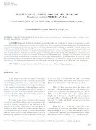
22 CHAPTER 2. CLASSICAL RESULTS ON CURVATURE LINESExample 2.2.2. Consider the family the one parameter of spheres defined byF(x,y,z,λ) = (x − λ) 2 + y 2 + z 2 − r 2 + λTherefore, F λ = −2(x − λ) + 1 = 0 and so the characteristic set is the hyperplane {x = 1/2 − λ}and the envelope is the paraboloid x = −(y 2 + z 2 ) + r 2 + 1/4.Example 2.2.3. Consider an one parameter family of spheres of constant radius r with centersin a curve c(s). So the family can be represented by F(p,s) = ‖p − c(s)‖ 2 − r 2 = 0. Therefore itfollows that F s = −2 〈p − c(s),c ′ (s)〉. The envelope of this family is called a canal surface.When c(s) = (R cos s,Rsins,0) the envelope is a torus of revolution that can be parametrizedby α(s,θ) = c(s) + r cos θ(cos s,sins,0) + r sin θ(0,0,1).Intuitively the envelope E is tangent to the family of surface defined F λ (p) = 0. More preciselythe following holdsProposition 2.2.1. Suppose that E is a regular surface and p ∈ E ∩ F −1λ(0). Then the tangentplane T p E coincides with the tangent plane of the surface F(p,λ) = 0.Proof. We leave to the reader.Proposition 2.2.2 (Vessiot). Consider the one parameter family of spheres with center c(s) andvariable radius r(s) > 0. Suppose that the envelope of this family is a regular surface. Then theenvelope can be parametrized byα(s,ϕ) = c(s) + r cos θ(s)T(s) + r(s)sin θ(s)[cos ϕN + sin ϕB]where cos θ(s) = −r ′ (s) and {T,N,B} is the Frenet frame of c. Moreover one family of linesof curvature are circles of radius r(s)sinθ(s) and the other is defined by the Riccati differentialequationdϕds= −τ(s) − k(s)cotg θ(s)sin ϕFigure 2.3: Canal surface with variable radiusProof. The family of spheres is defined byF(s,p) = |p − c(s)| 2 − r(s) 2 = 0

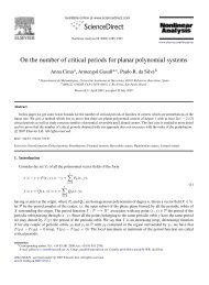
26 CHAPTER 2. CLASSICAL RESULTS ON CURVATURE LINES10) Show that a family of quadricsx 2a(u) + y2b(u) + z2c(u) − 1 = 0,where a, b and c are smooth functions, belongs to a triply orthogonal system of surfaces if and only ifthe following differential equation holdsa(b − c)a ′ + b(c − a)b ′ + c(a − b)c ′ = 0.(∗)Find special solutions of the differential equation above.Suggestion: Show that the solutions of the systemaa ′ = ah + g, bb ′ = bh + g, cc ′ = ch + g,where h = h(u) and g = g(u) are arbitrary smooth funcionts, are solutions of (*). See [23].11) Show that the system given byx 2 + y 2 + z 2 = ux, z = vy, (x 2 + y 2 + z 2 ) 2 = w(y 2 + z 2 )defines a triply orthogonal system of surfaces. Visualize the shape of the surfaces.12) Show that a triply orthogonal system is given by:i) the hyperbolic paraboloids yz = ux,ii) the closed sheets of the surface(y 2 − z 2 ) 2 − 2a(2x 2 + y 2 + z 2 ) + a 2 = 0,iii) the open sheets of the same surface.13) Consider the surface S parametrized by (u, v, h(u, v) where,h(u, v) = 1 2 (au2 + bv 2 ) + 1 6 (Au3 + 3Bu 2 v + 3Cuv 2 + Dv 3 )+ 124 (αu4 + 4βu 3 v + 6γu 2 v 2 + 4εuv 3 + δv 4 ) + · · ·(∗∗)Let c = c(s) be a principal curvature line of S passing through 0 and tangent to axis u. Let k and τbe, respectively, the curvature and the torsion of c at 0. Show thatk 2 τ =(3a − b)AB − 3aBC(a − b) 2 − αβa − b .Find the correspondent relation for the other principal curvature line and also determine the geodesiccurvatures of both principal lines at 0.14) Let S be the surface parametrized equation (**) above. Write the series of Taylor of the principalcurvatures k 1 = k 1 (u, v) and k 2 = k 2 (u, v) at 0 up to order two and analyse the level sets of bothfunctions near 0, imposing generic conditions on the coefficients (a, b, . . .,ε, δ).

Chapter 3Global Principal StabilityIntroductionIn this chapter we formulate and discuss the Global Principal Stability result for principalconfigurations of curvature lines.The results of this chapter are due to C. Gutierrez and J. Sotomayor, [38], [39] and [42].For a history about the theory of qualitative theory of principal lines see [72, 73] and for arecent survey see [34].3.1 Lines of curvature near Darbouxian umbilicsIn this section it will be reviewed the behavior of curvature lines near Darbouxian umbilics.3.1.1 Preliminaries concerning umbilic pointsDenote by PM 2 the projective tangent bundle over M 2 , with projection Π. For any chart (u,v)on an open set U of M 2 there are defined two charts (u,v;p = dv/du) and (u,v;q = du/dv) whichcover Π −1 (U).The differential equation (1.9) of principal lines, being quadratic, is well defined in the projectivebundle. Thus, for every α in I r ,L α = {τ g,α = 0, }defines a variety on PM 2 , which is regular and of class C r−2 over M 2 \ U α . It doubly covers M 2 \ U αand contains a projective line Π −1 (p) over each point p ∈ U α .Definition 3.1.1. A point p ∈ U α is Darbouxian if the following two conditions hold:T : The variety L α is regular also over Π −1 (p). In other words, the derivative of τ g,α does notvanish on the points of projective line Π −1 (p). This means that the derivative in directionstransversal to Π −1 (p) must not vanish.27

28 CHAPTER 3. GLOBAL PRINCIPAL STABILITYD : The principal line fields L i,α , i = 1,2 lift to a single line field L α of class C r−3 , tangent to L α ,which extends to a unique one along Π −1 (p), and there it has only hyperbolic singularities,which must be eitherD 1 : a unique saddleD 2 : a unique node between two saddles, orD 3 : three saddles.For calculations it will be essential to express the Darbouxian conditions in a Monge local chart(u,v): (M 2 ,p) → (R 2 ,0) on M 2 , p ∈ U α , as follows.Take an isometry Γ of R 3 with Γ(α(p)) = 0 such that Γ(α(u,v)) = (u,v,h(u,v)), withh(u,v) = k 2 (u2 + v 2 ) + (a/6)u 3 + (b/2)uv 2 + (b ′ /2)u 2 v+(c/6)v 3 + (A/24)u 4 + (B/6)u 3 v(3.1)+(C/4)u 2 v 2 + (D/6)uv 3 + (E/24)v 4 + O((u 2 + v 2 ) 5/2 ).To obtain simpler expressions assume that the coefficient b ′ vanishes.This is achieved by means of a suitable rotation in the (u,v)-plane.In the affine chart (u,v; p = dv/du) on P(M 2 ) around Π −1 (p), the variety L α is given by thefollowing equation.T (u,v,p) = L(u,v)p 2 + M(u,v)p + N(u,v) = 0, p = dv/du. (3.2)The functions L, M and N are obtained from equation (1.9) and (3.1) as follows:L = h u h v h vv − (1 + h 2 v)h uvM = (1 + h 2 u )h vv − (1 + h 2 v )h uuN = (1 + h 2 u )h uv − h u h v h uu .Calculation taking into account the coefficients in equation 3.1, with b ′ = 0, gives:L(u,v) = − bv − (B/2)u 2 − (C − k 3 )uv − (D/2)v 2 + M 3 1 (u,v)M(u,v) =(b − a)u + cv + [(C − A)/2 + k 3 ]u 2 + (D − B)uv(3.3)+[(E − C)/2 − k 3 ]v 2 + M2(u,v)3N(u,v) =bv + (B/2)u 2 + (C − k 3 )uv + (D/2)v 2 + M3 3 (u,v),with M 3 i (u,v) = O((u2 + v 2 ) 3/2 ), i = 1, 2, 3.These expressions are obtained from the calculation of the coefficients of the first and secondfundamental forms in the chart (u,v). See also [16, 38, 42]. With longer calculations, Darboux [16]gives the full expressions for any value of b ′ .Remark 3.1.2. The regularity condition T in definition 3.1.1 is equivalent to impose that b(b −a) ≠ 0. In fact, this inequality also implies regularity at p = ∞. This can be seen in the chart(u,v; q = du/dv), at q = 0.Also this condition is equivalent to the transversality of the curves M = 0, N = 0

3.1. LINES OF CURVATURE NEAR DARBOUXIAN UMBILICS 29The line field L α is expressed in the chart (u,v; p) as being generated by the vector field X = X α ,called the Lie-Cartan vector field of equation (1.9), which is tangent to L α and is given by:˙u =∂T /∂p˙v =p∂T /∂p(3.4)ṗ = − (∂T /∂u + p∂T /∂v)Similar expressions hold for the chart (u,v;q = du/dv) and the pertinent vector field Y = Y α .The function T is a first integral of X = X α . The projections of the integral curves of X α byΠ(u,v,p) = (u,v) are the lines of curvature. The singularities of X α are given by (0,0,p i ) wherep i is a root of the equation p(bp 2 − cp + a − 2b) = 0.Assume that b ≠ 0, which occurs under the regularity condition T, then the singularities of X αon the surface L α are located on the p-axis at the points with coordinates p 0 , p 1 , p 2p 0 =0,p 1 =c/2b − √ (c/2b) 2 − (a/b) + 2,p 2 =c/2b + √ (c/2b) 2 − (a/b) + 2(3.5)Remark 3.1.3. [38] Assume the notation established in equation (3.1). Suppose that the transversalitycondition T : b(b − a) ≠ 0 of definition 3.1.1 and remark 3.1.2 holds. Let ∆ = −[(c/2b) 2 −(a/b)+2]. Calculation of the hyperbolicity conditions for singularities (3.5) of the vector field (3.4)–see [38]– have led to establish the following equivalences:D 1 ) ≡ ∆ > 0D 2 ) ≡ ∆ < 0 and 1 < a b ≠ 2D 3 ) ≡ a b < 1.See Figs. 3.2 and 3.1 for an illustration of the three possible types of Darbouxian umbilics. Thedistinction between them is expressed in terms of the coefficients of the 3-jet of equation (3.1), aswell as in the lifting of singularities to the surface L α . See remarks 3.1.2 and 3.1.3.The subscript i = 1,2,3 of D i denotes the number of umbilic separatrices of p. These areprincipal lines which tend to the umbilic point p and separate regions of different patterns ofapproach to it. For Darbouxian points, the umbilic separatrices are the projection into M 2 of thesaddle separatrices transversal to the projective line over the umbilic point.It can be proved that the only umbilic points for which α ∈ I r is locally C s -structurally stable,r > s ≥ 3, are the Darbouxian ones. See [45, 42].The implicit surface T (u,v,p) = 0 is regular in a neighborhood of the projective line if andonly if b(b − a) ≠ 0. Near the singular point p 0 = (0,0,0) of X α it follows that T v (p 0 ) = b ≠ 0 andtherefore, by the Implicit Function Theorem, there exists a function v such that T (u,v(u,p),p) = 0.The function v = v(u,p) has the following Taylor expansionv(u,p) = − B 2b u2 + a − b up + O(3).b

30 CHAPTER 3. GLOBAL PRINCIPAL STABILITYFigure 3.1: Darbouxian Umbilic Points, corresponding L α surface and lifted line fields.For future reference we record the expression the vector field X α in the chart (u,p).˙u =T p (u,v(u,p),p)[b(C − A + 2k 3 ) − cB]u 2 +b=(b − a)u + 1 2ṗ = − (T u + pT v )(u,v(u,p),p) =−Bu + (a − 2b)p − cp 2 + 1 [B(C − k 3 ) − a 41 b]u 22 b+ [b(A − C − 2k3 ) + a(k 3 − C)]up + O(3),bc(a − b)up + O(3)bwhere a 41 is ∂5 h∂u 4 ∂v , evaluated at (0,0). However, a 41 will have no influence in the qualitative analysisthat follows.Theorem 3.1.4 (Gutierrez, Sotomayor, 1982). Let p an umbilic point of an immersion α given ina Monge chart (u,v) by:Suppose the following conditions:T) b(b − a) ≠ 0α(u,v) = (u,v, k 2 (u2 + v 2 ) + a 6 u3 + b 2 u2 v + c 6 v3 + o(4))D 1 ) ( c 2b )2 − a b + 2 < 0D 2 ) ( c2b )2 + 2 > a b > 1, a ≠ 2baD 3 )b < 1Then the behavior of lines of curvature near the umbilic point p, in the cases D 1 , D 2 and D 3 ,called Darbouxian Umbilics, is as in the Fig. 3.2An immersion α ∈ M r , r ≥ 4, is C 3 − principally structurally stable at a point p ∈ U α if only if pis a Darbouxian umbilic point.(3.6)Remark 3.1.5. The description of the curvature lines near umbilic points of analytic surfaces wasperformed by G. Darboux, [16]. He used the techniques of ordinary differential equations developedby H. Poincaré. For C k ,k ≥ 4, surfaces this analysis was done by Gutierrez and Sotomayor [38]and also by Bruce and Fidal [45].

3.2. HYPERBOLIC PRINCIPAL CYCLES 31Figure 3.2: Lines of Curvature near Darbouxian Umbilic Points3.2 Hyperbolic Principal CyclesA closed line of principal curvature is called a principal cycle.A principal cycle called hyperbolic if the first derivative of the Poincaré map associated to it isdifferent from one.Lemma 3.2.1. Given a biregular closed curve c : [0,l] → R 3 parametrized by arc length s. Let kand τ the curvature and the torsion of c. Then there exists a surface containing c as a principalcycle if and only if ∫ l0τ(s)ds = 2kπProof. Let {t,n,b} the Frenet frame associated to c. Write the normal vector of the surface in theform N = cos θ(s)n(s) + sin θ(s)b(s).Therefore N ′ (s) ∧ t = 0 ( Rodrigues equation of curvature lines) if and only if θ ′ + τ(s) = 0. Soθ(s) = θ 0 + ∫ s0 τ(u)du and N(θ(l)) = N(θ 0) if and only if ∫ l0τ(u)du = 2kπ, k ∈ Z.Lemma 3.2.2. Let c : [0,l] → M 2 be a principal cycle parametrized by arc length u and length l.Then the expression:α(u,v) = (α ◦ c)(u) + v(N ∧ t)(u) + [ k 22 v2 + A(u,v)v 2 ]N(c(u)) (3.7)where A(u,0) = 0 and k 2 is the principal curvature of α, defines a local chart of class C ∞ aroundc.Proof. Similar to lemma 5.1.1. The coefficient of v 2 stated in the lemma is given by k n (c(u),N ∧t) =k 2 (u).Proposition 3.2.1. Letc : [0,l] → M 2 be a principal cycle l parametrized by arc length u andof length l. Then the derivative of the Poincaré map Π, associated to it is given by:∫ llnΠ ′ −k 2′ (0) = du = 1 ∫dH√k 2 − k 1 2 H 2 − K0where H = k 1+k 22and K = k 1 k 2 are respectively the Mean Curvature and the Gaussian Curvature.Proof. The Darboux equations for the positive frame {t,N ∧ t,N} are:ct ′ (u) = k g (u)(N ∧ t)(u) + k 1 N(u)(N ∧ t) ′ (u) = −k g (u)t(u)N ′ (u) = −k 1 (u)t(u)(3.8)

32 CHAPTER 3. GLOBAL PRINCIPAL STABILITYby:Direct calculations gives that:e(u,0) = k 1 , f(u,0) = 0, g(u,0) = k 2 ,f v (u,0) = k ′ 2, F v (u,0) = 0, G(u,0) = E(u,0) = 1.The differential equation of the curvature lines in the neighborhood of the line {v = 0} is givenEf − Fe + (Eg − Ge) dv + (Fg − Gf)(dvdu du )2 = 0 (3.10)Denote by v(u,r) the solution of the 3.10 with initial condition v(0,r) = r. Therefore the returnmap Π is clearly given by Π(r) = v(L,r).Differentiating equation (3.10) with respect to r, and evaluating at v = 0, it results that:(3.9)[Eg − Ge](u,0)v ur (u,0) + [Ef − Fe] v (u,0)v r (u,0) = 0 (3.11)Therefore, using the expressions for [Ef − Fe] v (u,0) calculated in equation (3.9), integrationof equation (3.11) it is obtained:So,This ends the proof.lnΠ ′ (0) =∫ l02ln Π ′ (0) =−k 2′ ∫ l[du = − k′ 2 − ]k′ 1du − k′ 1duk 2 − k 1 0 k 2 − k 1 k 2 − k 1∫ l0− k′ 1 + k′ 2k 2 − k 1du =∫ l0H ′−√ H 2 − K duProposition 3.2.2. Let c : [0,l] → M 2 be a principal cycle parametrized by arc length u and lengthl. Suppose that dk 1 |c ≠ 0. Consider the deformationα ǫ (u,v) = α(u,v) + ǫ k′ 12 v2 δ(v)N(c(u)) (3.12)where δ is a smooth function with small support and δ|V 0 = 1. Then for all ǫ ≠ 0 small c is ahyperbolic principal cycle of α ǫ .Proof. Direct calculation shows that c is a principal cycle and thatTherefore,This ends the proof.Π ′ ǫ(0) = exp∫ l0k ′ 1− du.k 2 + ǫ − k 1dΠ ′ ∫ lǫ(0)(k 1 ′ | ǫ=0 = exp)2dǫ0 (k 2 − k 1 ) 2du ≠ 0.Proposition 3.2.3. Let c be a hyperbolic principal cycle of length l. Then there exists a principalchart (u,v), l−periodic in u such that differential equation of curvature lines in a neighborhood ofc is given bydu(dv − λdu) = 0,Rcλ = e− dk 2k 2 −k 1

3.3. A THEOREM ON PRINCIPAL STABILITY 33Proof. See [25] and [26].An immersion α ∈ M r is C s −Principally Structurally Stable at a principal cycle c if for everyneighborhood V c of c in M there must be a neighborhood V α of α in M k,s such that for every mapβ ∈ V α there must be a principal cycle c β in V c and a local homeomorphism h β on the domain suchthat h β : W c → W cβ between neighborhoods of c and c β , which maps c to c β and maps P 1,α |W cand P 2,α |W c respectively onto P 1,β |W cβ and P 2,β |W cβ .From the discussion above we have the following.Proposition 3.2.4 (Gutierrez, Sotomayor, 1982). An immersion α ∈ M r , r ≥ 4, is C 3 − principallystructurally stable at a principal cycle c provided one of the following equivalent conditions,H 1 or H 2 , is satisfied:∫dkH 1 ) 1c k 2 −k 1= ∫ dk 2c k 2 −k 1≠ 0H 2 ) The cycle is a hyperbolic principal cycle of the principal foliation which it belongs. That is, thePoincaré return map h associated to a transversal section to c at a point q is such that h ′ (q) ≠ 1.Remark 3.2.1. The higher derivatives of the Poincaré map Π near principal cycles was studiedin [40] and [25].3.3 A Theorem on Principal StabilityNext we will define the set S r (M) ⊂ M r such that:1. All the umbilic points, U α , of α are Darbouxian,2. All principal cycles of α are hyperbolic,3. The limit set of every principal line of α is the union of umbilic points and principal cycles,4. There is no umbilic or singular separatrix of α which is separatrix of two umbilic or twice aseparatrix of the same umbilic or singular point (i.e. homoclinic loops are not allowed).An immersion α ∈ M r is said to be C s −Principally Structurally Stable if there is a neighborhoodV α of α in M such that for every immersion β ∈ V α there exist a homeomorphism h β on the domainsuch that h β (U α ) = U β and h β maps lines of P 1,α , (resp. P 2,α ) on those of P 1,β ( resp. P 2,β .)Theorem 3.3.1 (Gutierrez, Sotomayor, 1982). Let r ≥ 4 and M be a compact oriented two manifold.Thena) The set S r (M) is open in M r,3 and every α ∈ S r (M) is C 3 -principally structurally stable.b) The set S r (M) is dense in M r,2 .A self sufficient presentation of this theorem was given in [42].3.4 Concluding RemarksAn open problem concerning the theorem 3.3.1 above is to prove (or disprove) that the setS r (M) is dense in M r,3 . The main point here is also related with the Closing-Lemma for PrincipalCurvature Lines.

34 CHAPTER 3. GLOBAL PRINCIPAL STABILITY3.5 Exercises1) Consider the singular cubic surface defined byf(x, y, z) = x2a 2 + y2b 2 − z2 + rxyz = 0, (a − b)r ≠ 0.i) Perform an analysis of the qualitative behavior of the principal foliations near the point (0, 0, 0).ii) Perform an analysis of the principal foliations near the ends of f −1 (0).Suggestion: Read the papers [27, 28].2) Give an explicit example of an algebraic surface having a hyperbolic principal cycle for each principalfoliation. Suggestion: See [28].3) Consider the cubic surfacef(x, y, z) = x2a 2 + y2b 2 + z2 + rxyz − 1 = 0, (a − 1)(b − 1)(a − b)r ≠ 0.i) For r ≠ 0 small make an analysis of the umbilic points of S = f −1 (0).ii) Make simulations (conjectures) about the possible global behavior of principal foliations of S.4) Consider the algebraic surfacef(x, y, z) = z 2 − [(x − 2a) 2 + y 2 − a 2 ][(x + 2a) 2 + y 2 − a 2 ][r 2 − x 2 − y 2 ] = 0, r > 4a.i) Determine the umbilic set of S = f −1 (0).ii) Determine all planar principal lines of S.iii) Using the symmetry of S try to obtain the global principal configuration of S.iv) Visualize the shape of S.5) Consider the space of quadrics Q in R 3 with the topology of coefficients. Define the concept ofstrucutural principal stability in this space.i) Determine the dimension of Q.ii) Characterize the quadrics which are principally stable.iii) Show that the set of quadrics structurally stable S 0 is open and dense in Q.iv) Characterize the connect components of S 0 .6) In the space of quadrics Q define the concept of first order structural principal stability. See [71, 69]to see the analogy with vector fields on surfaces.i) Characterize the quadrics which are first order principally stable.ii) Characterize the connect components of S 0 .iii) Characterize the set Q \ (S 0 ∪ S 1 ). Here S 1 is the set of quadrics which are first order principallystable.

3.5. EXERCISES 357) Consider the implicit differential equation(g − HG)dv 2 + 2(f − HF)dudv + (e − HE)du 2 = 0.Here H = (k 1 +k 2 )/2 is the arithmetic mean curvature. The integral curves of the equation above arecalled arithmetic curvature lines.i) Make a study of arithmetic curvature lines on the quadrics of R 3 .ii) Make an analysis of the arithmetic curvature lines near umbilic points and closed arithmetic curvaturelines. See [31, 32].

36 CHAPTER 3. GLOBAL PRINCIPAL STABILITY

Chapter 4Bifurcations of Umbilic Points andPrincipal Curvature LinesIntroductionThe local study of principal configurations around an umbilic point received considerable attentionin the classical works of Monge [24], Cayley [14], Darboux [16] and Gullstrand [1], amongothers.The study of the global features of principal configurations P α which remain topologically undisturbedunder small perturbations of the immersion α –principal structural stability– was initiatedby Gutierrez and Sotomayor in [38, 39, 42].Two generic patterns of bifurcations of umbilic points appear in codimension one. The firstone occurs due to the violation of the Darbouxian condition D, while T is preserved, leading tothe pattern called D2 1 . The second one happens due to the violation of condition T, leading to thepattern denominated D2,3 1 .This chapter is based in [61] and is restricted only to the simplest bifurcations of umbilic points.4.1 Umbilic Points of Codimension OneHere will be studied the qualitative changes - bifurcations - of the principal configurations aroundnon Darbouxian umbilic points such that the regularity (or transversality) condition T : b(a−b) ≠ 0,which implies their isolatedness, is preserved and only the condition D is violated in the mildestpossible way.Definition 4.1.1. A point p ∈ U α is said to be of type D 1 2if the following holds:T : The variety L α is regular also over Π −1 (p). In other words, the derivative of τ g,α does notvanish on the points of projective line Π −1 (p). This means that the derivative in directionstransversal to Π −1 (p) must not vanish.D2 1 : The principal line fields L i,α, i = 1,2 lift to a single line field L α of class C r−3 , tangent to L α ,which extends to a unique one along Π −1 (p), and there it has a hyperbolic saddle singularityand a saddle-node whose central manifold is located along the projective line over p.37

38 CHAPTER 4. BIFURCATIONS OF UMBILICSIn coordinates (u,v), as in the notation above, this means thatT : b(a − b) > 0 and either1) a/b = (c/2b) 2 + 2, or2) a/b = 2.We point out that due to the particular representation of the 3-jets taken here, with b ′ = 0, thespace a,b,c in the case 2) is not transversal, but tangent, to the manifold of jets with D 1 2 umbilics.Remark 4.1.2. The D2 1 umbilic point has two separatrices.The isolated one is characterized by the fact that no other principal line which approaches theumbilic point is tangent to it.The other separatrix, called non-isolated, has the property that every principal line distinct fromthe isolated one, that approaches the point does so tangent to it.These separatrices bound the parabolic sector of lines of curvature approaching the point; theyalso constitute the boundary of the hyperbolic sector of the umbilic point.The bifurcation illustrated in Fig. 4.1 shows that the non-isolated separatrix disappears whenthe point D 1 2 changes to D 1 and that it turns into an isolated D 2 separatrix when it changes intoD 2 . It can be said that D 1 2 represents the simplest transition between D 1 and D 2 Darbouxianumbilic points, which occurs through the annihilation of an umbilic separatrix – the non-isolatedone –.The coefficients of the differential equation of principal curvature lines (1.9) are given by:with M 3 i (u,v) = O((u2 + v 2 ) 3 2).L(u,v) = − bv − (B/2)u 2 − (C − k 3 )uv − (D/2)v 2 + M 3 1 (u,v)M(u,v) =(b − a)u + cv + [(C − A)/2 + k 3 ]u 2 + (D − B)uv(4.1)+[(E − C)/2 − k 3 ]v 2 + M2(u,v)3N(u,v) =bv + (B/2)u 2 + (C − k 3 )uv + (D/2)v 2 + M3 3 (u,v),Condition D 1 2 is equivalent to the existence of a non zero double root for bp2 − cp + a − 2b = 0,which amounts to b ≠ 0 and p 1 = p 2 ≠ p 0 .Assuming b(b − a) ≠ 0, the curves L = 0 and M = 0 meet transversally at (0,0) if and only ifb ≠ a. It was shown in [38] that D 1 is satisfied if and only if the roots of bp 2 − cp + a − 2b = 0 arenon vanishing and purely imaginary.Also, D 2 is satisfied if and only if bt 2 − ct + a − 2b = 0 has two distinct non zero real roots,p 1 , p 2 which verify p 1 p 2 > −1.This means that the rays tangent to the separatrices are pairwise distinct and contained in anopen right angular sector.The local configuration of D2 1 is established now.Proposition 4.1.1. Suppose that α ∈ I r ,r ≥ 5, satisfies condition D2 1 at an umbilic point p. Thenthe local principal configuration of α around p is that of Fig. 4.1 center.Proof. Consider the Lie-Cartan lifting X α as in equation (3.4), which is of class C r−3 . If a = 2b ≠ 0and c ≠ 0, it follows that p 0 = (0,0,0) is an isolated singular point of quadratic saddle node type

4.1. UMBILIC POINTS OF CODIMENSION ONE 39with a center manifold contained in the projective line –the p axis–. In fact, the eigenvalues ofDX α (0) are λ 1 = −b ≠ 0 and λ 2 = 0 and the p axis is invariant; there X α , according to equation(3.6) is given by ṗ = −cp 2 + o(2).The other singular point of X α is given by p 1 = (0,0, c b). It follows that⎡ ⎤−b −c 0⎢ ⎥DX α (0,0,p 1 ) = ⎣−c − c2 b0 ⎦where,A 1 A 2c 2 bA 1 = b2 c(A − k 3 − 2C) + bc 2 (2B − D) + c 3 (C − k 3 ) − b 3 Db 3A 2 = b2 c(B − 2D) + bc 2 (2C + k 3 − E) + b 3 (k 3 − C) + Dc 3b 3The non zero eigenvalues of DX(0,0,p 1 ) are λ 1 = c2 b , λ 2 = − c2 +b 2b. In fact, p 1 is a hyperbolicsaddle point of X α having eigenvalues given by λ 1 and λ 2 .Similar analysis can be done when ( c2b )2 − a b + 1 = 0. In this case X α and p 1 = (0,0, c b ) is aquadratic saddle node, with a local center manifold contained in the projective line. The pointp 0 = (0,0,0) is a hyperbolic saddle of X α . This case is equivalent to the previous one, after arotation in (u,v) that sends de saddle-node to p = 0.Proposition 4.1.2. Suppose that α ∈ I r ,r ≥ 5, satisfies condition D2 1 at an umbilic point p. Thenthere is a function B of class C r−3 on a neighborhood V of α and a neighborhood V of p such thatevery β ∈ V has a unique umbilic point p β in V .i) dB(α) ≠ 0ii) B(β) > 0 if and only if p β is Darbouxian of type D 1iii) B(β) < 0 if and only if p β is Darbouxian of type D 2iv) B(β) = 0 if and only if p β is of type D 1 2The principal configurations of β around p is that of Fig. 4.1, left, right and center, respectively.Figure 4.1: Umbilic Point D 1 2and bifurcationProof. Since p is a transversal umbilic point of α, the existence of the neighborhoods V and V ofp β follow from the Implicit Function Theorem. So we assume that after an isometry Γ β of R 3 , with

40 CHAPTER 4. BIFURCATIONS OF UMBILICSΓ β β(0) = 0, in the neighborhood V are defined coordinates (u,v), also depending on β, on whichit is represented as:h β (u,v) = k β2 (u2 + v 2 ) + a β6 u3 + b β2 uv2 + c β6 v3 + O(β;(u 2 + v 2 ) 4 ).Define the functionB(β) = [ c β] 2 − a β+ 2,2b β b βwhose zeros define locally the manifold of immersions with a D 1 2 point.The derivative of this function in the direction of the coordinate a is clearly non-zero.4.1.1 The D 1 2,3Umbilic Bifurcation PatternThe second case of non-Darbouxian umbilic point studied here, called D2,3 1 , happens when theregularity condition T is violated.Definition 4.1.3. An umbilic point is said of type D2,3 1 if the transversality condition T fails attwo points over the umbilic point, at which L α is non-degenerate of Morse type.Proposition 4.1.3. Suppose that α ∈ I r , r ≥ 5, and p be an umbilic point. Assume the notationin equation (3.1) with b ′ = 0, b = a ≠ 0 and b(C − A + 2k 3 ) − cB ≠ 0.right.Then p is of type D 1 2,3and the local principal configuration of α around p is that of Fig. 2,Proof. Consider the Lie-Cartan lifting X α as in equation (3.4), which is of class C r−3 . Imposinga = b ≠ 0, by equations (3.5) and (3.6), the singular points of X α are p 0 , p 1 and p 2 , roots of theequation p(bp 2 − cp − b) = 0.In fact, if a = b ≠ 0, it follows that p 0 is a quadratic saddle node with center manifold transversalto the projective line.From equation (3.6) the eigenvalues are λ 1 = 0 and λ 2 = −b and all the center manifolds W care tangent to the line p = − B b u. By invariant manifold theory it follows that X|W c is locallytopologically equivalent towhere,It follows that˙u = 1 2[b(C − A + 2k 3 ) − cB]u 2 + o(2) := − χ b2b u2 + o(2). (4.2)⎡⎤0 −2bp i + c 0⎢⎥DX α (0,0,p i ) = ⎣ 0 −p i (2bp i − c) 0 ⎦B 1 B 2 3bp 2 i − 2cp i − bB 1 =(C − k 3 )p 3 i + (2B − D)p 2 i + (A − 2C − k 3 )p i − BB 2 =Dp 3 i + (2C + k3 − E)p 2 i + (B − 2D)p i + k 3 − C.The nonzero eigenvalues of DX α (0,0,p i ) are λ 1 = −2bp 2 i + cp i = −b(p 2 i + 1) and λ 2 = 3bp 2 i −2cp i − b = b(p 2 i + 1).

4.1. UMBILIC POINTS OF CODIMENSION ONE 41Figure 4.2: Lie-Cartan suspension D 1 2,3By invariant manifold theory, (0,0,p i ) are saddles of X α . The phase portrait of X α near thesesingularities are as shown in Fig. 4.2.The two critical points p 1 and p 2 are of conic type on the variety L α over the umbilic point.These points are non-degenerate or of Morse type, according to the analysis below. At thepoints (0,0,p i ) the variety T (u,v,p) = 0 is not regular. In fact:∇T (0,0,p) = [(b − a)p, −bp 2 + cp + b,0].Therefore, for a = b ≠ 0, at the two roots of the equation −bp 2 + cp + b = 0 it follows that∇T (0,0,p i ) = (0,0,0),i = 1,2.The Hessian of T at p i = (0,0,p i ) isHess(T )(p i ) =⎡⎢⎣p i (−cB+b(C+2k 3 −A))bp i (c(k 3 −C)+b(D−B)b− p i(cD+b(C−E+2k 3 ))bp i (c(k 3 −C)+b(D−B))b0⎥c − 2bp i ⎦ .0 c − 2bp i 0Direct calculation, using the notation defined in equation (4.2), givesdet(Hess(T )(0,0,p i )) = p i(−2bp i + c) 2 χb= p ib (4b2 + c 2 )χ ≠ 0.Therefore, (0,0,p i ) is a non degenerate critical point of T of Morse type and index 1 or 2 –acone–, since T −1 (0) contains the projective line.Remark 4.1.4. Our analysis has shown the equivalence between the conditions a) and b) thatfollow:a) The non-vanishing on the Hessian of T on the critical points p 1 and p 2 over the umbilic.b) The presence of a saddle-node at p 0 on the regular portion of the surface L α , with centralseparatrix transversal to the projective line over the umbilic.⎤

42 CHAPTER 4. BIFURCATIONS OF UMBILICSFurther direct calculation with equation 4.1 gives that these two conditions are equivalent toc) The quadratic contact at the umbilic between the curves M = 0 and N = 0.In fact, from equation (4.1) it follows that M(u,v(u)) = 0 for v = −(B/2b)u 2 + o(2) of classC r−2 . Therefore n(u) = N(u,v(u)) is of class C r−2 and n(u) = −(χ/2b)u 2 + o(2).Notice also that, unlike the other umbilic points discussed here, the two principal foliationsaround D2,3 1 are topologically distinct.One of them, located on the parallel sheet, has two umbilic separatrices and two hyperbolicsectorsThe other, located on the saddle-node sheet, has three umbilic separatrices, one parabolic andtwo hyperbolic sectors.The separatrix which is the common boundary of the hyperbolic sectors will be called hyperbolicseparatrix. See Figs. 3.1, 4.1 and Fig. 4.2 for illustrations.The bifurcation analysis describes the elimination of two umbilic points D 2 and D 3 which, undera deformation of the immersion, collapse into a single umbilic point D2,3 1 , and then, after a furthersuitable arbitrarily small perturbation, the umbilic point is annihilated.Proposition 4.1.4. Suppose that α ∈ I r ,r ≥ 5, satisfies condition D2,3 1 at an umbilic point p.Then there is a function B of class C r−3 on a neighborhood V of α and a neighborhood V of p suchthati) dB(α) ≠ 0ii) B(β) > 0 if and only if β has no umbilic points in V ,iii) B(β) < 0 if and only if β has two Darbouxian umbilic points of types D 2 and D 3 ,iv) B(β) = 0 if and only if β has only one umbilic point in V , which is of type D 1 2,3 .The principal configurations of β around p are illustrated in Fig. 4.3, right, left and center,respectively.Proof. Similar to that given in [69], page 15, for the saddle-node of vector fields, using the equivalencec) of remark 4.1.4. We define B as follows. An immersion β in a neighborhood V of α anda neighborhood V of p can be written in a Monge chart as a graph of a function h β (u,v). Theumbilic points of β are defined by the equationM β = (1 + ((h β ) u ) 2 )(h β ) vv − (1 + ((h β ) v ) 2 )(h β ) uu = 0N β = (1 + ((h β ) u ) 2 )(h β ) uv − (h β ) u (h β ) v (h β ) uu = 0.For β in a neighborhood of α it follows that M β (u,v β (u)) = 0.Define B(β) = n β (u β ), where u β is the only critical point of n β (u) = N β (u,v β (u)).Taking h β (u,v) = h(u,v) + λuv, where h is as in equation (3.1) it follows by direct calculationthat dB(β)dλ | λ=0 ≠ 0.The bifurcation of the point D2,3 1 can be regarded as the simplest transition between umbilicsD 2 and D 3 and non umbilic points. See the illustration in Fig. 4.3.(4.3)

4.2. EXERCISES 43Figure 4.3: Umbilic Point D 1 2,3and bifurcation.4.2 Exercises1) Define suitable deformations of the surface f(x, y, z) = x 4 + y 4 + z 4 − 1 = 0 such that the resultantsurface has exactly 20 Darbouxian umbilics, 8 of type D 3 and 12 of type D 1 .2) Consider the cubic surface defined byi) Write the equation of umbilic points of f −1 (0).ii) Determine the Darbouxian umbilics of f −1 (0).f(x, y, z) = x 2 + y 2 + z 2 + rxyz − 1 = 0, r ≠ 0.3) Make a study of principal curvature lines near non hyperbolic principal cycles and give an example ofa surface having a semihyperbolic principal cycle. See [40] and [25].4) Determine the principal configuration of the map α(u, v) = (u, uv, v 2 ) near the Whitney singular point(0, 0). See [60].5) Give examples of smooth surfaces having separatrix connections (homoclinic and heteroclinic) betweenDarbouxian umbilic points. For example in the ellipsoid we have connections between separatrices ofDarbouxian umbilics of type D 1 . See [41].6) Give examples of smooth surfaces having lines of umbilic points and analyse the behavior of principallines near these lines. See [33].7) Give an example of a surface,homeomorphic to S 2 , having exactly one singular and no umbilic points.8) Give an example of a canal surface, homeomorphic to the torus, having no umbilic points, one prinipalfoliation having all principal lines closed and other principal foliation having all principal lines dense.8) Consider the surfacesf(x, y, z) = x2a 2 + y2b 2 + z2x2− 1 = 0, g(x, y, z) =c2 A 2 + y2B 2 − z2C 2 − 1 = 0.Suppose that f −1 (0) ∩ g −1 (0) is the union of principal curvature lines on both surfaces.Analyse the behavior of the principal foliations of the surface defined by h ǫ (x, y, z) = f(x, y, z)g(x, y, z)−ǫ = 0 for ǫ ≠ 0 small. Visualise the shape of h ǫ −1(0).Make simulations in a free software disponible in the homepage of A. Montesinos (Univ. Valencia,Espanha), http://www.uv.es/montesin

44 CHAPTER 4. BIFURCATIONS OF UMBILICS

Chapter 5Structural Stability of AsymptoticLinesIntroductionIn this chapter it will be considered the simplest qualitative properties of the nets defined bythe asymptotic lines of a surface immersed in Euclidean space.Asymptotic lines are defined only in the hyperbolic part of the surface, where two real asymptoticdirections are defined. In the elliptic region the asymptotic directions are complex. At aparabolic point, if not planar, we have only one asymptotic direction with multiplicity two.Conditions for local structural stability around parabolic points and periodic asymptotic linesare established. This chapter is based mainly in [26] and [59]. The global theory of structuralstability of the nets of asymptotic lines was developed in [59].5.1 Asymptotic Nets near Parabolic pointsIn this section it will be established the behavior of the asymptotic nets near parabolic points,in terms of geometric invariants of the immersion α.Let c : [0,L] → M 2 be a regular arc of parabolic points, parametrized by arc length u. Tofix the notation, suppose that k 2|c = 0 and k 1|c < 0, where k 1 and k 2 are the principal curvaturesof the immersion α. Let ϕ(u) the angle between c ′ (u) = t(u) and the principal direction L 2 (α),corresponding to k 2 , at the point c(u). Denote by k g (u) the geodesic curvature of c at the pointc(u).The following lemma will be useful in what follows.Lemma 5.1.1. Let c : [0,L] → M 2 be a regular arc of parabolic points, parametrized by arclength u. Then the expression:α(u,v) = (α ◦ c)(u) + v(N ∧ t)(u) + [k ⊥ n (u)v 2 /2 + v 2 A(u,v)]N(c(u)) (5.1)where, A(u,0) = 0 and k ⊥ n (u) = k n (c(u),N ∧ t(u)), defines a local chart of class C ∞ around c.45

46 CHAPTER 5. STABILITY OF ASYMPTOTIC LINESProof. The map α(u,v,w) = (α ◦c)(u)+v(N ∧t)(u)+wN(u) is a local diffeomorphism. Therefore,solving the equation 〈α(u,v,w(u,v)),N(u)〉 = 0 and using the Hadamard lemma it follows theresult asserted.5.1.1 Computation of the Second Fundamental FormIn what follows it will be calculated the coefficients and the derivatives of the second fundamentalform of α in the chart introduced in 5.1.1.Calculations in the chart (u,v)The Darboux equations for the positive frame {t,N ∧ t,N} are:⎧t ⎪⎨′ (u) = k g (u)(N ∧ t)(u) + k n (u)N(u)(N ∧ t) ′ (u) = −k g (u)t(u) + τ g (u)N(u)⎪⎩(N) ′ (u) = −τ g (u)(N ∧ t)(u) − k n (u)t(u)(5.2)with τg 2 (u) = kn ⊥ (u)k n (u). This is because c is a parabolic curve.Also, using Euler’s formula, [75], [17], it follows that, kn ⊥ = k 1 cos 2 ϕ, k n = k 1 sin 2 ϕ , kn ⊥ +k n =2H and τ g = k 1 sin ϕcos ϕ.For the sake of simplicity in the expressions that follow, writeA = A(u,v),N = (N ◦ c)(u),kn ⊥ = k (u),k g = k g (u)Moreover the following notation will be used:E = 〈α u ,α u 〉 e = 〈α u ∧ α v ,α u 〉F = 〈α u ,α v 〉 f = 〈α u ∧ α v ,α v 〉G = 〈α v ,α v 〉 g = 〈α u ∧ α v ,α v 〉Here E,F,G and e/ | α u ∧ α v |, f/ | α u ∧ α v | and g/ | α u ∧ α v | are respectively thecoefficients of the first and second fundamental forms of α, expressed in the chart(u,v).Differentiating equation (5.1) and using equation (5.2), obtain:α u = [1 − k g v − k n (k ⊥ n+ [τ g v + (k ⊥ n )′v22 + v2 A u ]Nv 22 + v2 A)]t − τ g (kn⊥ v 22 + v2 A)N ∧ t(5.3)α v = N ∧ t + (k ⊥ n v + 2vA + v 2 A v )N (5.4)α u ∧ α v = −[τ g v + (k ⊥ n )′ v 2 + v 2 A u + τ g (k ⊥ n− [(1 − k g v − k n (k ⊥ n[1 − k g v − k n (k ⊥ nv 22 + v2 A)(k ⊥ n v + 2vA + v2 A v )]tv 22 + v2 A))(k ⊥ n v + 2vA + v 2 A v )]N ∧ tv 22 + v2 A)]N(5.5)

5.1. PARABOLIC POINTS 47α uu = [−k g ′ v − k n((kn ⊥ )′v22 + v2 A u ) − k n ′ v 2(k⊥ n2 + v2 A)− k n (τ g v + (k ⊥ n )′v22 + v2 A u ) + k g τ g (k ⊥ n+ [k g (1 − k g v − k n (k ⊥ nv 22 + v2 A)]tv 22 + v2 A)) − τ g (τ g v + (k ⊥ n ) ′v22 + v2 A u )− τ ′ g((k ⊥ n ) v22 + v2 A) − τ g ((k ⊥ n ) ′v22 + v2 A u )]N ∧ t+ [k n (1 − k g v − k n (k ⊥ n+ τ ′ gv + (k ⊥ n ) ′′v22 + v2 A uu ]Nv 22 + v2 A)) − τ 2 g (k ⊥ nα uv = −[k g + k n (k ⊥ n v + 2vA + v 2 A v )]t+ [τ g + (k ⊥ n )′ v + 2vA u + v 2 A uv )]N− τ g (k ⊥ n v + 2vA + v2 A v )N ∧ tv 22 + v2 A)(5.6)(5.7)From equations (5.3) to (5.8) it results thatα vv = [k ⊥ n + 2A + 4vA + v2 A vv ]N (5.8)e(u,0) = k n (u) = k 1 sin 2 ϕf(u,0) = τ g (u) = k 1 sinϕcos ϕg(u,0) = k ⊥ n (u) = k 1 cos 2 ϕe v (u,0) = −k g (2k n + k ⊥ n ) + τ ′ gf v (u,0) = (k ⊥ n ) ′(5.9)g v (u,0) = −k g k ⊥ n + 6A vE v (u,0) = −2k g , F v (u,0) = 0, G v (u,0) = 0From the relation, 2H(EG − F 2 ) 3 2 = eG − 2fF + gE and equation (5.9) it follows that,6A v (u,0) = 2H v − 6k g H + k g (2k n + 4kn ⊥ ) − τ g ′ (5.10)Also, from K(EG − F 2 ) 2 = eg − f, and equations (5.9) and (5.10), it is obtained that,K v (u,0) = k g [k1 2 cos 2ϕ − 2τg 2 ] + k 1 τ g ′ − 2τ g (kn ⊥ ) ′ − 2H v k n ≠ 0,which expresses the condition of regularity of the parabolic set in section 5.1.The main result of this section is formulated by the following,Proposition 5.1.1. Let c be a curve of parabolic points as above. Then the following holds:i) If ϕ(u) ≠ 0 the asymptotic net, near c(u), is as shown in 5.1 (cuspidal type).ii ) If ϕ(u) = 0 and ϕ ′ (u) ≠ 0 there are three cases:1. k g (u)/ϕ ′ (u) < 1,2. 1 < k g (u)/ϕ ′ (u) < 9

48 CHAPTER 5. STABILITY OF ASYMPTOTIC LINES3. 9 < k g (u)/ϕ ′ (u).In cases 1), 2) and 3) above the asymptotic net is as shown in the figure 5.1 and correspondrespectively to the folded saddle, node and focus types parabolic points.Figure 5.1: Asymptotic lines near a parabolic lineProof. The cuspidal case: transversal crossingSuppose that the principal foliation P 2 (α) is transversal to the parabolic line at the point u 0 ,this means that ϕ(u 0 ) ≠ 0.Using Hadamard lemma, write:e(u,v) = k n (u) + v[−k g (2k n + k ⊥ n ) + τ ′ g ] + vA 1(u,v),f(u,v) = τ g (u) + v(k ⊥ n ) ′ + v 2 A 2 (u,v),g(u,v) = k ⊥ n (u) + v[2H v − 6k g H + k g (2k n + 3k ⊥ n ) − τ ′ g ] + v2 A 3 (u,v),Then,with, k n (u) = k 1 sin 2 ϕ, k ⊥ n (u) = k 1 cos 2 ϕ, τ g (u) = k 1 sinϕcos ϕ.The differential equation of the asymptotic lines are given by:Let v = w 2 . So, it follows that,⎧⎪⎨edu 2 + 2fdudv + gdv 2 = 0du/dv = −f ± [f2 − eg] 1 2edudv = −2wf e ± 2w2 W(u,v)e⎪⎩ u(u 0 ,0) = u 0.where W(u,0) = [K v (u,0)] 1 20 by transversality conditions.Solving the Cauchy problem above it results that:u(u 0 ,v) = u 0 − cotgϕ(u 0 )v ± W(u 0 ,0)v 3 2 + ...Therefore near a cuspidal parabolic point the net of asymptotic lines is as shown in the Fig.5.1.

5.1. PARABOLIC POINTS 49Remark 5.1.1. It follows from [3] that there exist a system of coordinates (U,V ) near a cuspidalparabolic point such that the differential equation of the asymptotic lines is given by (dV/dU) 2 = U.The singular case: point of quadratic tangency.Now suppose that τ g (u 0 ) = 0,u 0 = 0. This means that the parabolic line is tangent to theprincipal foliation F 2 (α) at u 0 . In fact, at a parabolic point the principal direction corresponding tothe zero principal curvature is an asymptotic direction. Suppose also that at the point of tangencyu 0 the contact above is quadratic, which is expressed by the conditions τ g (0) = 0 and τ g ′ (0) ≠ 0.Consider the implicit differential equation,F(u,v,p) = e + 2fp + gp 2 = 0,and the line field given locally by the vector field X,⎧u ⎪⎨′ = F pX : v ′ = pF p⎪⎩p ′ = −(F u + pF v )p = dvduThe projections of the integral curves of X by Π(u,v,p) = (u,v) are the asymptotic lines of α.The singularities of X in F −1 (0) are given by: (u 0 ,0,0), where τ g (u 0 ) = 0. Suppose u 0 = 0.It results that the Jacobian matrix of DX(0) is given by:⎛2f u 2f v 2g⎜DX(0) = ⎝ 0 0 0−e uu −e uv −(2f u + e v )⎞⎟⎠ (5.11)Using equations (5.9) and (5.11) it results that the eigenvalues of DX(0) are given by:λ 1 ,The eigenspace associated to λ i is given by:λ 2 = ( k⊥ n2 ){(k g − ϕ ′ ) ± [(k g − ϕ ′ )(k g − 9ϕ ′ )] 1 2 }E i = (1,0, ϕ′4 [(a − 1) ± √ (a − 1)(a − 9) − 4])where a = kgϕ ′ .The tangent space of Π −1 (P ) ∩ F −1 (0) at the point (u 0 ,0,0) is generated by (1,0,0).Therefore E i is transversal to the singular set Π −1 (P α ) ∩ {F = 0}.In the case of the saddle point (λ 1 λ 2 < 0), although the eigenspaces have inclinations of samesign, that is, (λ 1 − 2k ⊥ n ϕ ′ )(λ 2 − 2k ⊥ n ϕ ′ ) > 0, the vector (1,0,0) bisects the acute angle formed byE 1 and E 2 . This implies that the net of asymptotic lines near a saddle folded parabolic point is asshown in Fig. 5.1.In the case of a focus singularity (λ 1 = ¯λ 2 , Re(λ 1 ) ≠ 0) the net of asymptotic lines is as shownin Fig. 5.1.In the case of a nodal singularity (λ 1 λ 2 > 0) the two eigenspaces also have inclinations of thesame sign, but here (1,0,0) bisects the obtuse angle formed by E 1 and E 2 . Also E 2 bisects the angleformed by (1,0,0) and E 1 (the tangent space to the strong separatrice). Therefore near a nodalfolded parabolic point the net of asymptotic lines is as shown in Fig. 5.1.

50 CHAPTER 5. STABILITY OF ASYMPTOTIC LINES5.2 Structural stability at parabolic pointsAn immersion α in I, is said to be C s -local asymptotic structurally stable, at p if it has aneighborhood N in the space I s such that for each β in N there is a smooth diffeomorphism k β of{M, NE α } to {M, NE } such that β ◦ k β is local asymptotic topologically equivalent to α at k β (p).Theorem 5.2.1. For an open and dense set W of immersions in I s ,s ≥ 5, the asymptotic netnear a parabolic point as described in proposition 5.1.1 are locally asymptotic stables.Proof. Follows from proposition 5.1.1 and by the main results of Bleeker and Wilson [10] andFeldman [21]. The construction of the topological equivalence, using the method of canonicalregions, can be done in the same way as in [59].5.3 Stability of Periodic Asymptotic LinesIn this section will be established an integral expression for the derivative of the first returnmap of a regular periodic asymptotic line in terms of curvature functions of the immersion α.Also, it will be shown how to deform the immersion in order to hyperbolize a regular or a foldedperiodic asymptotic line.5.3.1 Regular Periodic Asymptotic Lines.Recall that a regular periodic asymptotic line is a closed asymptotic line which is disjoint fromthe parabolic points.Lemma 5.3.1. Let c : [0,L] → M 2 be a periodic asymptotic line parametrized by arc length u andlength L. Then the expression:α(u,v) = (α ◦ c)(u) + v(N ∧ t)(u) + [H(u)v 2 + A(u,v)v 2 ]N(c(u)) (5.12)where A(u,0) = 0 and H is the Mean Curvature of α, defines a local chart of class C ∞ around c.Proof. Similar to lemma 5.1.1. The coefficient of v 2 stated in the lemma is given by k ⊥ n .Using that k n (u) = k n (c(u),t(u)) = 0 for an asymptotic line and applying Euler’s formulafollows that, k ⊥ n + k n = 2H.Proposition 5.3.1. Let c : [0,L] → M 2 be a regular periodic asymptotic line parametrized byarc length u and of length L. Then the derivative of the Poincaré map Π, associated to it is givenby:[∫ LΠ ′ (0) = exp0τ ′ g − 2k g (u)H(u)2τ g (u)where k g is the geodesic curvature of c and τ g = (−K) 1 2 is the geodesic torsion of c.]duProof. The Darboux equations for the positive frame {t,N ∧ t,N} are:

5.3. STABILITY OF PERIODIC LINES 51t ′ (u) = k g (u)(N ∧ t)(u)(N ∧ t) ′ (u) = −k g (u)t(u) + τ g (u)N(u)N ′ (u) = −τ g (u)(N ∧ t)(u)The same procedure of calculation used in the lemma 5.1.1 gives that:(5.13)e(u,0) = 0, e v (u,0) = τ g ′ − 2H(u)k g(u)(5.14)f(u,0) = τ g (u) g(u,0) = 2H(u)The differential equation of the asymptotic lines in the neighborhood of the line {v = 0} isgiven by:e + 2f dvdu + g(dv du )2 = 0 (5.15)Denote by v(u,r) the solution of the 5.15 with initial condition v(0,r) = r. Therefore the returnmap Π is clearly given by Π(r) = v(L,r).Differentiating 5.15 with respect to r, it results that:g r v r (dv/du) 2 + (2gv ur + 2f v v r )(dv/du) + e v v r = 0Evaluating at v = 0, it follows that:2f(u,0)v ur (u,0) + e v (u,0)v r (u,0) = 0 (5.16)Therefore, using the expressions for f an e v found in equation (5.14), integration of (5.16) it isobtained:This ends the proof.ln Π′(0) =∫ L0−τ g ′ + 2Hk gdu2τ gRemark 5.3.1. From [74, pp. 282] it follows thatis a 1-form evaluated along an asymptotic line.ω = τ ′ g − 2k g (u)H(u)2τ gProposition 5.3.2. Let c : [0,L] → M 2 be a regular periodic asymptotic line of length L, parametrizedby arc length u, of the immersion α.Consider the following one parameter deformation of α:α ǫ (u,v) = α(u,v) + ǫw(u)δ(v)v 2 N(u)where δ | c = 1 and has small support. Then c is a regular periodic asymptotic line of α ǫ for all ǫsmall and the derivative of the Poincaré map Π αǫ , associated to it is given by:[∫ LΠ ′ α ǫ= exp0]k g (u)[H(u) + ǫw(u)]du .τ g (u)

52 CHAPTER 5. STABILITY OF ASYMPTOTIC LINESMoreover, taking w(u) = k g (u) holds that:d (Π′dǫαǫ(0) ) ∫ Lk g (u) 2| ǫ=0 =0 τ g (u) du ≠ 0In particular c is a hyperbolic periodic asymptotic line for α ǫ ,ǫ ≠ 0.Proof. Performing the calculation as in Lemma 5.3.1 it follows that:e(ǫ,u,0) = 0, f(ǫ,u,0) = τ g (u),g(ǫ,u,0) = 2(H(u) + ǫw(u)),e v (ǫ,u,0) = −2[H(u) + ǫw(u)]k g (u) + τ ′ g (u).Therefore {v = 0} is a closed asymptotic line for α ǫ . So applying Proposition 5.3.1 to α ǫ anddifferentiating under the integration sign gives the result stated.Remark 5.3.2. In order see that k g | c is not identically zero for a periodic asymptotic line, weobserve that for an asymptotic line c, the geodesic curvature coincides with the ordinary curvatureof c, considered as a curve in E 3 . Therefore, if k g | c = 0, it follows that c must be a straight line.5.3.2 Folded periodic asymptotic linesHere will be established an integral expression for the derivative of the first return map of afolded periodic asymptotic line in terms of the curvature functions of the immersion α.A folded periodic asymptotic line is a closed asymptotic curve c : [0,L] → M regular by parts,that is, there exist a finite sequence of numbers a i ,0 = a 0 < a 1 < ... < a l = L, such thatc i = c | (ai ,a i+1: (a i ,a i+1 ) → IntH is an asymptotic line of α and p i = c(a i ) ∈ P α for i = 1,... ,l − 1.In other words, a folded periodic asymptotic line is the projection of a closed integral curve of thesingle line field L α defined on A, which intersects P α .Let c be a folded periodic asymptotic line. Near each point p i , consider two transversal sectionsto c,Σ 1,i and Σ 2,i , and the Poincaré map σ i : Σ 1,i → Σ 2,i . Denote by u j i = c i(a i ,a i+1 )∩Σ j,i ,j = 1,2.Denote by π i+1,i : Σ 2,i → Σ 1,i+1 the Poincaré map associated to c i . It follows that the Poincarémap associated to c,Π : Σ 1,1 → Σ 1,1 is given by:Π = π l−1,1 ◦ σ l−1 ... ◦ π i+1,i ◦ ... ◦ π 2,1 ◦ σ 1 .Proposition 5.3.3. Let c : [0,L] → M 2 be a folded periodic asymptotic line of length L parametrizedby arc length u. Assume the notation above. Then the derivative of the Poincaré map π i+1,iassociated to c i is given by:[ ∫ ]u 1i+1 −τ g(u) ′ + 2k g (u)H(u)π i+1,i (0) = expdu2τ g (u)u 2 iwhere k g is the geodesic curvature of c i and τ g = (−K) 1 2 is the geodesic torsion of c i . Moreover thefunctions σ i are differentiable.Proof. Near the point p i take a system of coordinates (U,V ) such that the asymptotic lines aregiven by the differential equation (dU/dV ) 2 = U. See [3], [6] and Remark 5.1.1.In this system of coordinates σ i : {V = ǫ} → {V = ǫ} is clearly a translation σ i (u,ǫ) = (u+c,ǫ).Therefore σ i is differentiable.

5.3. STABILITY OF PERIODIC LINES 53Figure 5.2: Folded periodic asymptotic lines5.3.1The expression for the derivative of π i+1,i can be obtained in the same way as in the PropositionProposition 5.3.4. Let c : [0,L] → M 2 be a folded periodic asymptotic line parametrized by arclength u and of length L. Assume the notation above.Consider the following one parameter deformation of α:α ǫ (u,v) = α(u,v) + ǫw(u)δ(v)vN(u)where δ | c = 1 and has small support and supp (δ) ∩ c(a i ,a i+1 ) ≠ ∅.Then c is a folded asymptotic line of α ǫ for all ǫ small and the derivative of the Poincaré mapπ αǫ,i+1,i associated to it is given by:[ ∫ ]u 1Π ′ α = exp i+1 −τ g(u) ′ + 2k g (u)[H(u) + ǫw(u)]ǫ,i+1,i du .2τ g (u)Moreover, taking w(u) = k g (u) holds that:u 1 iddǫ (π α ǫ,i+1,i(0)) | ǫ=0 =∫ u 1i+1u 2 ik g (u) 2τ g (u) du ≠ 0In particular c is a hyperbolic periodic asymptotic folded line for α ǫ , ǫ ≠ 0.Proof. Similar to the proof of proposition 5.3.2. Here one must take an arc which is not a straigthline.From the considerations above we have the following.Theorem 5.3.3. Given a regular or folded asymptotic periodic line c of the immersion α, thenthere exist a smooth one parameter family of immersions α t such that for t > 0 small, c is ahyperbolic asymptotic line of α t which is structurally stable.

54 CHAPTER 5. STABILITY OF ASYMPTOTIC LINES5.4 Examples of Periodic Asymptotic LinesIn this section it will be given geometric constructions of regular surfaces having periodic asymptoticlines.5.4.1 A Hyperbolic periodic asymptotic lineIn this subsection it will be considered a surface having a hyperbolic asymptotic line containedin interior of the region of negative Gaussian curvature.Proposition 5.4.1. Let c : [0,L] → R 3 be a closed biregular curve, parametrized by arc length,such that the curvature k(s) and the torsion τ(s) of c are different from zero for all s ∈ [0,L].Consider the surfaceα(s,v) = c(s) + vN(s) + τ(s) v22 B(s)Here {T,N,B} is Frenet’s orthonormal frame associated to c.Then c is a regular hyperbolic periodic asymptotic line.Proof. Direct calculation gives thate(s,0) = 0, f(s,0) = τ(s), e v (s,0) = τ ′ (s) − k(s)τ(s) g(s,0) = τ(s).The Poincaré map given by π(v 0 ) = v(L,v 0 ), where v is the solution of the differential equationeds 2 + 2fdsdv + gdv 2 = 0with v(0,v 0 ) = v 0 , has the first derivative at 0 given by:This ends the proof.π ′ (0) = exp∫ L0− e v2f (s,0)ds = exp ∫ L0k(s)2 ds ≠ 1Remark 5.4.1. Curves with the above propertied are, for example, the toroidal helices, [9]. Forappropriate pairs (m,n), the closed curve c m,n defined below has non zero torsion.c m,n (t) = ((R + r cos nt)cos mt,(R + r cos nt)sinmt,r sin nt)5.4.2 Semihyperbolic periodic asymptotic lineIn this section it will be considered a ruled surface having a non hyperbolic asymptotic linecontained in interior of the region of negative Gaussian curvature. Under an integral condition itwill be proved the semi hyperbolicity of a closed asymptotic line.Proposition 5.4.2. Let c : [0,L] → R 3 be a closed biregular curve, parametrized by arc length,such that the curvature k(s) and the torsion τ(s) of c are different from zero for all s ∈ [0,L].Consider the ruled surfaceα(s,v) = c(s) + vN(s)

5.4. EXAMPLES OF PERIODIC ASYMPTOTIC LINES 55Then c is a regular semi hyperbolic periodic asymptotic line provided∫τ −1/2 dk ≠ 0.Proof. Direct calculation gives thatα s ∧ α v = −τvT + (1 − vk)Bcα ss = −k ′ vT + [k − (k 2 + τ 2 )v]N + τ ′ Bα sv = −kT + τBα vv = 0Therefore e = [α ss ,α s ,α v ], f = [α sv ,α s ,α v ] and g = [α vv ,α s ,α v ] are given by.e(s,v) = τ ′ (s)v + ( k τ )′ (s)τ 2 v 2f(s,v) = τ(s)g(s,v) = 0Therefore one family of asymptotic lines is given by the straight lines s = cte and c is an asymptoticline of the other foliation. The Poincaré map associated to c is defined by π(v 0 ) = v(L,v 0 ), wherev = v(s,v 0 ) is the solution of the differential equationdvds = (s)v + ( k−τ′ τ )′ (s)τ 2 v 22τv(0,v 0 ) = v 0Direct integration of the first variational equationevaluated at v = 0 gives,Therefore,dds ( dvdv 0) = − τ ′2τdvdv 0√ √dv τ(0) τ0(s) = √ = √dv 0 τ(s) τπ ′ (0) = ∂v∂v 0(0,L) = 1Also, the integration of the second variational equation,d vds (d2 dv02 ) = − τ ′ d 2 v2τ dv02 − ( dv ) 2 ( k dv 0 τ )′ τleads toThis ends the proof.d 2 vdv 2 0∫ L √τ0= −0= − √ ∫τ 0 kd(τ −1/2 ) = √ ∫τ 0√ τ( k τ )′ τ(s)ds = − √ τ 0∫ Lcc0τ −1/2 dk√ τ(kτ )′ ds

56 CHAPTER 5. STABILITY OF ASYMPTOTIC LINES5.5 On a class of dense asymptotic linesThe goal of this section is to present examples of folded recurrent asymptotic lines.The goal of this section is to present examples of folded recurrent asymptotic lines.Proposition 5.5.1. Let T 2 be the torus of revolution, obtained by the rotation of the circle (x −R) 2 + z 2 = r 2 ,r < R, around the z axis. Then the qualitative behavior of the asymptotic lines is asshown in the figure 5.3 Moreover the return map Π : S(R) → S(R), where S(R) = {(x,y,z) :x 2 + y 2 = R 2 ,z = −r}, is a rotation by an angle equal to 4RT(r/R), whereT( r R ) = ∞ ∑n=02a nn! ( r 1 × 3 × . . . × (2n − 1) Γ( 1R )n 2, with a n = )Γ(2n + 1 4 )2 n Γ(2n + 3 4 ) .Figure 5.3: Asymptotic lines on the torusProof. Consider the following parametrization of the torus of revolution:(u,v) → (cos v(R + r cos u),sin v(R + r cos u),r sin u)Performing the calculation of the second fundamental form, it is obtained that,e(u,v) = R 2 , f(u,v) = 0, g(u,v) = R(R + r cos u)cos u.Therefore the differential equation of the asymptotic lines is:F(u,v,du/dv) = R(du/dv) 2 + cos u(R + r cos u) = 0.Writing p = du/dv, consider the vector field X defined by the differential equation(u ′ ,v ′ ,p ′ ) = (F p ,pF p , −(F u + pF v )).After multiplying X by 1/p it results that:(u ′ ,v ′ ,p ′ ) = (2Rp2R,Rsin u + r sin 2u).Consider also the projected vector field,{u ′ = 2RpY :p ′ = R sinu + r sin 2u

5.6. FURTHER DEVELOPMENTS ON ASYMPTOTIC LINES 57Notice that the orbit of Y through ( π 2 ,0) reaches (3π 2 ,0).In fact, from the first integral of Y ,G(u,p) = Rp 2 + R cos u + r cos 2u,2it follows that ( π 2 ,0) and (3π 2 ,0) are in the same connected component of G−1 ( −r2 ).The time spent by an orbit that starts at ( π 2 ,0) to reach the point (3π 2,0) can be calculated asfollows:As dudtFrom G(u,p) = r 2= 2Rp, it follows that:it results that:p = {[−r(1 + cos 2u) − 2R cos u]} 1 2 .2RT = R 1 2∫ 3π2π2du[− cos u(r cos u + R)] 1 2∫ π2= 20du[sin u(1 − r R sin .u)]1 2It follows from [36, pp. 369 –950], that the analytic function T( r R) has the following expansionin seriesT( r R ) = ∞ ∑n=02a nn! ( r 1 × 3 × . . . × (2n − 1) Γ( 1R )n 2, where a n = )Γ(2n + 1 4 )2 n Γ(2n + 3 4 ) .Therefore, from dv/dt = 2R, it follows that an arc of the asymptotic line that starts at the point( π 2 ,v 0) ends at the point ( 3π 2 ,v 1), where v 1 is given by v 1 = 2RT ∓ v.So the return map Π : {v = − π 2 } → {v = −π 2} is given byΠ(v 0 ) = v 0 + 4RT( r R ).As T is clearly non constant, it is possible to select r and R such that the rotation number ,see [54] and [53], of Π is irrational.5.6 Further developments on asymptotic linesThe geometric form described above was taken from [29].The local analysis of asymptotic lines near parabolic points was also studied in [7], [8] and [47].A global theorem of stability of nets of asymptotic lines was obtained in [59].The dynamical aspects of asymptotic lines is a source of many difficult problems.One is the “Closing Lemma”, i.e. the elimination of recurrent asymptotic lines disjoint fromthe parabolic set and of folded recurrent asymptotic lines.The second kind of recurrences was given by torus of revolution, see section 5.5.The first kind of recurrences was studied by R. Garcia and J. Sotomayor [35] in embedded torusof S 3 with suitable deformations of the Clifford torus.Another problem is about the existence of isolated regular closed asymptotic lines in tubes andalso a continuum of closed asymptotic lines. This kind of question is important in the open problemof rigidity of compact surfaces of genus different from zero and also in the study of complete surfaceswith negative Gaussian curvature.

58 CHAPTER 5. STABILITY OF ASYMPTOTIC LINESAnother kind of question is about the structure of the parabolic set of a surface, for example,in surfaces which are graph (x,y,p(x,y) of a polynomial p ∈ R[x,y].A concrete question is the following: Given a function K which local and global conditionsthis function must satisfies in order that K −1 = 0 is the parabolic set of a surface with Gaussiancurvature K? This question was considered by V. Arnold,[5].For compact surfaces, the function K must satisfy preliminarily the equation established by theGauss-Bonnet Theorem5.7 Exercises1) Consider the embedded tube defined by∫SKdS = 2πχ(S).α(s, v) = c(s) + r cosvn(s) + r sin vb(s), r > 0.Here c is a closed Frenet curve with k > 0 and torsion τ.i) Show that the hyperbolic region of α is diffeomorphic to a cylinder and the parabolic set is union oftwo regular curves.ii) Characterize the parabolic points (regular, folded saddle, etc.) in terms of (k, τ) and their derivatives.iii) Examine the possible global behavior of asymptotic foliations in the tube.iv) Let c be a connected component of f −1 (0)∩g −1 (0), where f(x, y, z) = x 2 +y 2 +z 2 −1 and g(x, y, z) =x 2a+ y22 b− 1. Classify the parabolic points of the tube with center c.22) Consider the surface S defined by the graph of the polynomial p(x, y) = k 2 (x2 + y 2 ) + x 3 − 3xy 2 .i) Determine the parabolic set of S.ii) Classify the parabolic points of S.iii) Examine the global behavior of asymptotic foliations on S, including the behavior near the infinity.3) Give examples of surfaces (try algebraic) such that:i) The parabolic set is the union of two regular curves and the hyperbolic region is diffeomorphic to acylinder.ii) The parabolic set is the union of three regular curves and the hyperbolic region is diffeomorphic to anoriented boundary surface S with Euler characteristic equal to ψ(S) = −1.iii) The parabolic set is a regular curve and the hyperbolic region is diffeomorphic to a disk.4) Show that the quartic algebraic surface defined byp(x, y, z) = 3z 4 + 2(1 + 4xy)z 2 − 2(x 2 + y 2 ) 2 + 8xy − 1 = 0,determines a smooth negatively curved surface S ⊂ R 3 homeomorphic to the doubly punctured torus,which has Euler characteristic equal to −2.i) Perform a qualitative analysis of the asymptotic foliations near the ends of p −1 (0).ii) Visualize the shape of p −1 (0).

5.7. EXERCISES 59Suggestion: See [15].5) Analyze the behavior of asymptotic lines near the Whitney singularities of an immersion of a surfacein R 3 . Suggestion: See [78].6) Let N : S → S 2 be the normal map associated to a surface S ⊂ R 3 . Classify the parabolic points ofS in terms of the singularities (folds and cusps) of N. See [7] and [8].7) Let α : S → S 3 be a smooth immersion of a surface S.. Define the first and second fundamentalforms of α with respect to the metric of S 3 induced by the canonical metric of R 4 and to the normalN α = (α u ∧ α v ∧ α)/|α u ∧ α v ∧ α|.A curve c : I → S is called an asymptotic line if II α (c(s))(c ′ (s), c ′ (s)) = 0i) Let α : S 1 × S 1 → S 3 defined byThe surface α(S 1 × S 1 ) is the Clifford torus..α(u, v) = 1 √2(cosu, sin u, cosv, sin v).i) Write the differential equation of asymptotic lines of α.ii) Show that the asymptotic lines of the Clifford torus are defined globally and are circles.8) Let α : S → R 4 be a smooth immersion of a compact two dimensional surface S and suppose thatthere exists a unitary normal vector field N α along α.Define the second fundamental form of α relative to N α by the equationII α (u, v)(du, dv) = 〈 D 2 α(u, v)(du, dv) 2 , N α〉= 〈α vv , N α 〉dv 2 + 2 〈α uv , N α 〉dudv + 〈α uu , N α 〉du 2=edu 2 + 2fdudv + gdv 2 .Make a study of the asymptotic lines of α relative to N α defined by the equation edu 2 +2fdudv+gdv 2 =0.9) Give an example of a ruled surface in R 3 having two hyperbolic asymptotic lines.10) Consider the parametric surface defined byx(u, v) = 12A [(a + u)3 + (a + v) 3 ]y(u, v) = 12B [(b + u)3 + (b + v) 3 ]z(u, v) = 12C [(a + c)3 + (a + c) 3 ]Obtain the differential equation of asymptotic lines and show that the solutions are given by11) Consider the parametric surface defined byu + ±v = c.x(u, v) =A(u − a) m (v − a) my(u, v) =B(u − b) m (v − b) mz(u, v) =C(u − c) m (v − c) m , m ∈ N.Obtain the differential equation of the asymptotic lines and find the solutions.

60 CHAPTER 5. STABILITY OF ASYMPTOTIC LINES12) Show that there is no triple system of surfaces cutting mutually in the asymptotic lines of thesesurfaces. See [19].13) Consider the ”osculator” tube defined byα(s, v) = c(s) + r cosvt(s) + r sin vn(s), r > 0.Here c is a Frenet curve with k > 0 and torsion τ and {t, n, b} is the Frenet frame.i) Characterize the curves c such that the ”osculator” tube defined above is a regular surface.ii) Analyse the geometry of the tube, classifying the elliptic, parabolic and hyperbolic points and alsothe singular points.ii) Analyse the principal and asymptotic lines of the tube.14) Make a study of extrinsic geometry of surfaces of codimension two in R 4 . In particular analyse theasymptotic lines, mean directionally curved lines and axial curvature lines. See [12], [30], [52], [63]and [64].

Chapter 6Closed Geodesics on SurfacesIntroductionGeometrical and dynamical aspects of geodesics on surfaces is a classical subject of differentialgeometry. See for example, [2], [4], [9], [16], [46], [49], [56], [57], [76], [77].In this chapter the derivative of the Poincaré map associated to a closed geodesic line will beobtained in a elementary way.6.0.1 Closed GeodesicsLemma 6.0.1. Let c : I → M 2 be a closed geodesic line parametrized by arc length. Then theDarboux frame is given by:T ′= k n N(N ∧ T) ′ = τ g NN ′ = −k n T − τ g N ∧ T(6.1)Moreover, τ g = (k 2 −k 1 )sin θ cos θ and k n = k 1 cos 2 θ+k 2 sin 2 θ, where k 1 and k 2 are the principalcurvatures and θ is the angle between c ′ (u) = T(u) and the principal direction corresponding to theprincipal curvature k 1 .Proof. From the Euler equation k n = k 1 cos 2 θ + k 2 sin 2 θ. Also the geodesic torsion given by τ g =(k 2 − k 1 )sin θ cos θ.Lemma 6.0.2. Let α : M → R 3 be an immersion of class C k , k ≥ 4, and c be a closed geodesiccurve of α, parametrized by arc length and of length l. Then the expression,α(u,v) = c(u) + v(N ∧ T)(u) + [k ⊥ n (u)v2 2 + A(u,v)v3 6 ]N(u),defines a local chart (u,v) of class C k−5 in a neighborhood of c.Proof. The curve c is of class C k−1 and the map α(u,v,w) = c(u)+v(N ∧T)(u)+wN(u) is of classC k−2 and is a local diffeomorphism in a neighborhood of the axis u. In fact [α u ,α v ,α w ](u,0,0) = 1.Therefore there is a function W(u,v) of class C k−2 such that α(u,v,W(u,v)) is a parametrizationof a tubular neighborhood of α ◦ c. Now for each u, W(u,v) is just a parametrization of the curve61

62 CHAPTER 6. CLOSED GEODESICSof intersection between α(M) and the normal plane generated by {(N ∧ T)(u),N(u)}. This curveof intersection is tangent to (N ∧ T)(u) at v = 0 and notice that kn ⊥ = k n(N ∧ T)(u). Therefore,α(u,v,W(u,v)) = c(u) + v(N ∧ T)(u) + [ k⊥ n2v 2 + A(u,v) v3 6 ]N(u),where A is of class C k−5 . This ends the proof.In the chart (u,v) constructed above it is obtained:E(u,v) = 1 + (τ 2 g − k nk ⊥ n )v2 + h.o.tF(u,v) = k ⊥ n τ v22 + h.o.tG(u,v) = 1 + (k ⊥ n )2 v 2 + h.o.te(u,v) = k n + h.o.tf(u,v) = τ g (u) + h.o.tg(u,v) = k ⊥ n + h.o.t(6.2)where in the expressions above, E = 〈α u ,α u 〉, F = 〈α u ,α v 〉, G = 〈α v ,α v 〉, e = 〈α u ∧ α v ,α uu 〉,f = 〈α u ∧ α v ,α uv 〉 and g = 〈α u ∧ α v ,α vv 〉.Therefore the Christoffel symbols are given by:Γ 1 11 = o(v 2 ), Γ 1 12 = v(τ2 g − k n k ⊥ n ) + o(v 2 ), Γ 1 22 = k⊥ n τ g v + o(v 2 )Γ 2 12 = o(v 2 ), Γ 2 11 = v(k nk ⊥ n − τ2 g ) + o(v2 ), Γ 2 22 = (k⊥ n )2 v + o(v 2 )(6.3)So the differential equation of geodesic lines is given by:dvdu= wdwdu= [k n τ g w 3 − k 2 n w2 + (τ 2 g − k nk ⊥ n )]v + o(v2 )(6.4)Proposition 6.0.1. Let α : M → R 3 be an immersion of class C k , k ≥ 4, and c be a closedgeodesic curve of α, parametrized by arc length and of length l. Then the derivative of the Poincarémap π(v 0 ,w 0 ) = (v(l,v 0 ,w 0 ),w(l,v 0 ,w 0 )) at (v 0 ,w 0 ) = (0,0) associated to equation (6.4) satisfiesthe following linear system:∂∂uMoreover det(π ′ (0)) = 1.(∂v∂v 0∂w∂v 0)∂v∂w 0∂w∂w 0=(0 1−K(u) 0)(∂v∂v 0∂w∂v 0)∂v∂w 0∂w∂w 0Proof. Direct calculation shows that K = k n kn ⊥−τ2 g . Therefore differentiating 6.4 the result follows.The assertion that det(π ′ (0)) = 1 it follows from Liouville formula for flows, [70].Proposition 6.0.2. Let α : M → R 3 be an immersion of class C k , k ≥ 4, and c be a closed geodesiccurve of α, parametrized by arc length and of length l. Suppose that K| c = k 0 . Then detπ ′ (0) = 1and the eigenvalues of π ′ (0) are given by λ 1 = − √ −k 0 and λ 2 = √ −k 0 . Therefore if k 0 < 0 theperiodic geodesic line c is hyperbolic and if k 0 > 0 the closed geodesic is simple.Proof. The result follows from the direct integration of linear system with constant coefficients6.5.(6.5)

636.0.2 Geodesics on Surfaces of RevolutionLet c : R → R 3 , c(u) = (r(u),0,z(u)), be a regular curve parametrized by arc length andconsider the surface of revolutionα(u,v) = (r(u)cos v,r(u)sin v,z(u)).The first fundamental form is given by: I α = ds 2 = du 2 + r(u) 2 dv 2 .The Christoffel symbols are given by:Γ 1 11 = 0 Γ 2 11 = 0Γ 1 12 = 0 Γ 2 12 = Gu2G = r′rΓ 2 11 = 0 Γ 1 22 = −G u = −2r ′ r(6.6)Therefore the differential equation of the geodesic lines is given by:d 2 uds 2d 2 vds 2−G u ( dvds )2 = 0+ Gu du dvG ds ds = 0ds 2 = du 2 + r(u) 2 dv 2 .From the second equation above it follows that:(6.7)d 2 vds 2ds = − G u dudvG ds dsdsTherefore integrating the equation above it results that,G dvds = cWriting the unitary tangent vector to the geodesic c(s) = (u(s),v(s)) in the form c ′ (s) =(cos β(s),sin β(s)), where β is the angle of the geodesic c with the meridians it follows that:flow.G dvds = r(u(s))2 sin β(s) = cThis relation is called Clairaut formula and it corresponds to a first integral of the geodesicSubstituting the Clairaut’s formula in the equation for ds 2 it results,c 2 du 2 + G(c 2 − G)dv 2 = 0 (6.8)The solutions of the binary equation above are the geodesics contained in the level set of the firstintegral G dvds = c.Proposition 6.0.3. Let u 0 be a parallel such that G(u 0 ) = c 2 . Then the following holds:1. If u = u 0 is not a geodesic then the behavior of equation (6.8) near u = u 0 is as shown in thepicture 6.1 a).2. The parallel u = u 0 is a geodesic if and only if u 0 is a critical point of r(u). Moreover, u = u 0is a minimum of r the behavior of the differential equation 6.8 near the parallel {u = u 0 } isas shown in the picture 6.1 b) below.

64 CHAPTER 6. CLOSED GEODESICSFigure 6.1: Geodesics on the surfaces of revolutionProof. Consider the implicit surfaceF(v,u,p) = c 2 p 2 + r(u) 2 (c 2 − r(u) 2 ) = 0,p = dudvThe Lie-Cartan vector field X = (F p ,pF p , −(F v + pF u )) is equivalent (modulus division by p)to the vector field Y given by:v ′ = 2c 2u ′ = 2c 2 pp ′ = −r ′ (u)r(u)(2c 2 − 4r(u) 2 )If r(u 0 ) = c and r ′ (u 0 ) = 0 it follows that curve ϕ(t) = (2c 2 t + v 0 ,u 0 ,0) is an integral solutionof the equation above with initial condition (v 0 ,u 0 ,0).If r(u 0 ) = c and r ′ (u 0 ) ≠ 0 it follows that curve ϕ(t) = (u 0 + 2c 2 t + · · · ,v 0 + 2r ′ (u 0 )c 5 t 2 +· · · ,2r ′ (u 0 )c 3 t + · · · ) is an integral solution of Y , with initial condition (v 0 ,u 0 ,0). Therefore theprojection of this integral curve on the plane vu has quadratic contact with the parallel {u = u 0 }.This ends the proof.6.0.3 Remarks on the Geodesic Flow on a SphereThe geodesic flow on a sphere S n is described by a second order differential equationu ′′ = λuAs 〈u,u ′ 〉 = 0 it follows that 〈u ′′ ,u〉+〈u ′ ,u ′ 〉 = 0 and that λ = −|u ′ | 2 . Therefore the differentialequation of the geodesic flow on a sphere is given by:u ′′ = −|u ′ | 2 u (6.9)Considering the function H(u,v) = 1 2 |u|2 |v| 2 , restricted to the tangent bundle given by {(u,v) :|u| = 1, 〈u,v〉 = 0}, the equation (6.9) is given by the Hamiltonian vector field˙u = ∂H∂v˙v = − ∂H∂uDirect analysis shows that all the geodesic lines of equation (6.9) are closed.The dynamics of the geodesic flow in convex hypersurfaces close to the unitary sphere is extremelyrich and it is an important area of research.For an analysis of the geodesic flow near closed geodesics on Riemannian manifolds see [80].

6.1. EXERCISES 656.1 Exercises1) Show that the ellipsoidx 2a 2 + y2b 2 + z2c 2 − 1 = 0, 0 < a < b < chas three closed planar geodesics. Discuss the type of each closed planar geodesic (elliptic or hyperbolic).ii) Show that there are closed geodesics of arbitrary length in the ellipsoid of revolution a = b < c.iii) Show that there are closed geodesics of arbitrary length in the ellipsoid of three different axes 0 < a

66 CHAPTER 6. CLOSED GEODESICS15) Consider the semi-plane R 2 + = {(u, v) : v > 0} with the metric ds 2 = du 2 + 1vdv 2 . Determine the2geodesics of R 2 + with respect to this metric.16) Make a study of various geometrical variational problems. For example, consider the following functional∫F(c) = k(s) 2 ds, s is the arc lengthin the space of regular curves with positive curvature kwith end points fixed.Determine the critical points of F.cC = {c : [a, b] → R 3 , c(a) = c a , c ′ (a) = c 1 a , c(b) = c b, c ′ (b) = c 1 b }17) Give an example of a real analytic Moebius band with Gauss curvature negative in R 3 and havingclosed geodesics.18) Give an example of a real analytic developable Moebius band in R 3 and having closed geodesics.

Bibliography[1] Gullstrand A. Zur kenntiss der kreispunkte. Acta Math, 29, 1905.[2] D. Anosov. Geodesic flows on closed riemmannian manifolds of negative curvature. Proc. SketlovInstitute of Mathematics. Amer. Math Soc. Transl. 1969., 90:209 pp., 1967.[3] V. Arnold. Geometrical Methods in the Theory of Ordinary Differential Equations. Springer-Verlag,1983.[4] V. Arnold. Mathematical Methods of Classical Mechanics. Springer-Verlag, 1989.[5] V. Arnold. On the problem of realization of a given gaussian curvature function. Topol. MethodsNonlinear Analysis, 11:199–206, 1998.[6] V. Arnold and Eds. Y. Iliashenko. Soviet Encyclopedia of Dynamical Systems, volume 01. Springer-Verlag.[7] T. Banchoff, T. Gaffney, and C. McCroy. Cusps of Gauss Maps, volume 55. Pitman Res. Notes inMath, 1982.[8] T. Banchoff and R. Thom. Sur les points paraboliques d’une surface: erratum et complements. C.R.Acad. Sc.Paris, Serie A, 291:503–505, 1981.[9] M. Berger and B. Gostiaux. Introduction to Differential Geometry. Springer-Verlag, 1987.[10] D. Bleeker and L. Wilson. Stability of gauss maps. Illinois J. Math., 22:279 – 289, 1978.[11] F. Mercuri C. Gutierrez and S. Bringas. On a conjecture of carathéodory: Analyticity versus smoothness.Experimental Mathematics, 5:33–37, 1996.[12] R. Tribuzy V. Guíñez C. Gutierrez, I. Guadalupe. Lines of curvature on surfaces immersed in R 4 . Bol.Soc. Brasil. Mat., 28:233–251, 1997.[13] C. Camacho and A. L. Neto. Introdução a Teoria Geométrica das Folheações. Projeto Euclides, CNPq,IMPA, 1981.[14] A. Cayley. On differential equations and umbilici. Philos. Mag., Coll. Works, Vol. VI, 26:373 – 379,441 – 452, 1863.[15] Chris Connel and Mohammad Ghomi. Topology of negatively curved real affine algebraic surfaces.www.math.gatech.edu/ ghomi/Papers/, page 27 pages, 2007.[16] G. Darboux. Leçons sur la théorie générale des surfaces, volume I, IV. Gauthiers-Villars, Paris, 1896.[17] M. do Carmo. Differential Geometry of curves and surfaces. Prentice Hall, New Jersey, 1976.[18] M. do Carmo. Geometria Riemanniana. Projeto Euclides, IMPA, 1988.[19] L. P. Eisenhart. A demonstration of the impossibility of a triply asymptotic system of surfaces. Bull.Amer. Math. Soc., 07:184–186, 1901.67

68 BIBLIOGRAPHY[20] L. P. Eisenhart. A Treatise on Differential Geometry of Curves and Surfaces. Dover Publications, Inc.,1950.[21] E. Feldman. On parabolic and umbilic points on hypersurfaces. Trans. Amer. Math. Soc., 127:1–28.[22] G. Fischer. Mathematical Models. Vieweg, 1986.[23] A. R. Forsyth. <strong>Lectures</strong> on the Differential Geometry of Curves and Surfaces. Cambridge Univ. Press,1920.[24] Monge G. Sur les lignes de courbure de la surface de l’ellipsoide. Journ. Ecole Polytech., II cah.[25] R. Garcia and J. Sotomayor. Lines of curvature near principal cycles. Annals of Global Analysis andGeometry, 10:199–218, 1992.[26] R. Garcia and J. Sotomayor. Lines of curvature near hyperbolic principal cycles. Pitman ResearchNotes in Mathematics Series, Edited by R. Bamon, R. Labarca, J. Lewowicz and J. Palis, 285:255–262,1993.[27] R. Garcia and J. Sotomayor. Lines of curvature near singular points of implicit surfaces. Bulletin deSciences Mathematiques, 117:313–331, 1993.[28] R. Garcia and J. Sotomayor. Lines of curvature on algebraic surfaces. Bulletin des Sciences Mathematiques,120:367–395, 1996.[29] R. Garcia and J. Sotomayor. Structural stability of parabolic points and periodic asymptotic lines.Matemática Contemporânea, Soc. Bras. Matemática, 12:83–102, 1997.[30] R. Garcia and J. Sotomayor. Lines of axial curvature on surfaces immersed in R 4 . Differential Geometryand its Applications, 12:253–269, 2000.[31] R. Garcia and J. Sotomayor. Structurally stable configurations of lines of mean curvature and umbilicpoints on surfaces immersed in R 3 . Publ. Matemátiques, 45:431–466, 2001.[32] R. Garcia and J. Sotomayor. Lines of mean curvature on surfaces immersed in R 3 . Qualit. Theory ofDyn. Syst., 5:137–183, 2004.[33] R. Garcia and J. Sotomayor. On the patterns of principal curvature lines around a curve of umbilicpoints. Anais da Acad. Brasileira de Ciências, 77:13–24, 2005.[34] R. Garcia and J. Sotomayor. Lines of curvature on surfaces, historical comments and recent developments.São Paulo Journal of Math. Sciences, 2:40, 2008.[35] R. Garcia and J. Sotomayor. Tori embedded in S 3 with dense asymptotic lines. Preprint, page 7, 2008.[36] I. Gradshteyn and I. Ryzhik. Table of Integrals, Series and Products. Academic Press, 1965.[37] W. Guilfoyle B., Klingenberg. On the space of oriented affine lines in R 3 . Archiv Math., 82:81–84, 2004.[38] C. Gutierrez and J. Sotomayor. Structurally stable configurations of lines of principal curvature. Asterisque,98-99:195–215, 1982.[39] C. Gutierrez and J. Sotomayor. An approximation theorem for immersions with structurally stableconfigurations of lines of principal curvature. Springer Lect. Notes in Math, 1007:332 – 368, 1983.[40] C. Gutierrez and J. Sotomayor. Closed lines of curvature and bifurcation. Bol. Soc. Bras. Mat., 17:1–19,1986.[41] C. Gutierrez and J. Sotomayor. Periodic lines of curvature bifurcating from darbouxian umbilicalconnections. Lect. Notes in Math., 1455:196–229, 1990.

BIBLIOGRAPHY 69[42] C. Gutierrez and J. Sotomayor. Lines of Curvature and Umbilic Points on Surfaces, Brazilian 18 thMath. Coll., IMPA, 1991, Reprinted as Structurally Configurations of Lines of Curvature and UmbilicPoints on Surfaces, Monografias del IMCA. Monografias del IMCA, Lima, Peru, 1998.[43] D. Hilbert and S. Cohn Vossen. Geometry and the Imagination. Chelsea, 1952.[44] H. Hopf. Differential Geometry in the Large, volume 1000. <strong>Lectures</strong> Notes in Math. Springer Verlag,1979.[45] J. Bruce J. and D. Fidal. On binary differential equations and umbilics. Proc. Royal Soc. Edinburgh,111A:147–168, 1989.[46] A. Katok and B. Hasselblatt. Introduction to the Modern Theory of Dynamical Systems, volume 54.Cambridge Univ. Press, 1995.[47] Y. Kergosian and R. Thom. Sur les points paraboliques des surfaces. Compt. Rendus Acad. Scien.Paris, 290,A:705–710, 1980.[48] W. Klingenberg. A Course in Differential Geometry, volume 51. Springer-Verlag, Graduate Texts,1978.[49] W. Klingenberg. Riemannian Geometry. Walter de Gruyter, 1982.[50] M. Fernández L. Cordero and A. Gray. Geometria diferencial de curvas y superficies. Addison-WesleyIberoamericana, 1995.[51] R. Langevin. Set of Spheres and Applications. XIII Escola de Geometria Diferencial, USP, 2004.[52] L. F. Mello. Mean directionally curved lines on surfaces immersed in R 4 . Publ. Mat., 47:415–440.[53] W. Melo and J. Palis. Introdução aos Sistemas Dinâmicos. Projeto Euclides, CNPq, IMPA, 1977.[54] W. Melo and S. van Strien. One Dimensional Dyanamics. Springer Verlag, 1993.[55] G. Monge. Journ. de l’Ecole Polytech, II e , 1796, Applications de l’Algebre a la Geometrie. Paris, 1850.[56] V. Ovskienko and T. Tabachnikov. Projective Differential Geometry Old and New. Cambridge UniversityPress, 2005.[57] H. Poincaré. Sur les lignes géodésiques sur les surfaces convexes. Trans. of Amer. Math. Society,06:237–274, 1905.[58] Porteous I. R. Geometric Differentiation. Cambridge University Press, 1994.[59] C. Gutierrez R. Garcia and J. Sotomayor. Structural stability of asymptotic lines on surfaces immersedin R 3 . Bulletin des Sciences Mathématiques, 123:599–622, 1999.[60] C. Gutierrez R. Garcia and J. Sotomayor. Lines of principal curvature around umbilics pand whitneyumbrellas. Tôhoku Mathematical Journal, 52:163–172, 2000.[61] C. Gutierrez R. Garcia and J. Sotomayor. Bifurcations of umbilic points and related principal cycles.Journ. Dyn. and Diff. Eq., 16:321–346, 2004.[62] J. Llibre R. Garcia and J. Sotomayor. Lines of principal curvature on canal surfaces in R 3 . Anais daAcad. Brasileira de Ciências, 78:405–415, 2006.[63] L. F. Mello R. Garcia and J. Sotomayor. Principal mean curvature foliations on surfaces immersed inR 4 . EQUADIFF 2003 World Sci. Publ., Hackensack, NJ, pages 939–950, 2006.[64] Maria A. S. Ruas R. Garcia, D.K H. Mochida; M. El Carmem R Fuster. Inflection points and topologyof surfaces in 4-space. Trans of Amer. Math. Society, 352:3029–3043, 2000.

70 BIBLIOGRAPHY[65] N. George R. Garcia and R. Langevin. Holonomy of a foliation by principal curvature lines. Bull. ofBraz. Math. Soc., 39:to appear, 2008.[66] A. Ros and S. Montiel. Curves and Surfaces. Grad. Studies in Math. 69, Amer.. Math. Society, 2005.[67] W. Chen S. Chern and K. Lam. <strong>Lectures</strong> on Differential Geometry, volume 01. World Scientific, 1999.[68] M. Salvai. On the geometry of the space of oriented lines in euclidean space. Manuscripta Math.,118:181–189.[69] J. Sotomayor. Generic one parameter families of vector fields on two dimensional manifolds. Publ.Math. I.H.E.S, 43:5–46.[70] J. Sotomayor. Lições de Equações Diferenciais Ordinárias. Projeto Euclides, CNPq, IMPA, 1979.[71] J. Sotomayor. Curvas Definidas por Equações Diferenciais no Plano. Brazilian 13 th Math. Coll., IMPA,1981.[72] J. Sotomayor. O elipsóide de monge. Matemática Universitária, 15:33–47, 1993.[73] J. Sotomayor. El elipsoide de monge y las líneas de curvatura. Materials Matematics, Jornal Eletrônico,Universitat Aut. de Barcelona, 1:1–25, 2007.[74] M. Spivak. A Comprehensive Introduction to Differential Geometry, volume III. Publish of Perish,Berkeley, 1979.[75] D. Struik. <strong>Lectures</strong> on Classical Differential Geometry. Addison Wesley, 1950, Reprinted by Dover,New York, 1988.[76] T. Tabachnikov. Projectively equivalent metrics, exact transverse line fields and the geodesic flow onthe ellipsoid. Comment. Math. Helv., 74:306–321.[77] F. Takens. Hamiltonian systems: Generic propeties of closed orbits and local perturbations. Math.Ann., 188:304–312, 1970.[78] F. Tari. On pairs of geometric foliations on a cross-cap. Tohoku Math. Journal, 59:233–258, 2007.[79] E. Vessiot. Leçons de Géometrie Supérieure. Librarie Scientifique J. Hermann, Paris, 1919.[80] F.Takens W. Klingenberg. Generic properties of geodesic flows. Comm. Math. Helvetica, 197:323–334,1972.[81] C. E. Weatherburn. On lamé families of surfaces. Ann. of Math., 28:301–308, 1926/27.

Indexasymptoticconfiguration, 14directions, 14folded line, 52foliations, 14line fields, 14nets, 45asymptotic linehyperbolic , 54semi hyperbolic , 54folded, 52dense, 56periodic, 50Bonnet coordinates, 15Clairaut formula, 63Closing-Lemma, 33curvaturesgeodesic, 11maximal, 13minimal, 13Darboux equationsasymptotic line, 46geodesic, 61principal lines, 31Differential EquationsAsymptotic Lines, 13Codazzi , 12Curvature Lines, 12Geodesics, 14Ricatti , 23Rodrigues, 13fundamental formfirst, 9second, 10Gauss map, 15geodesicflow , 64lines, 14principally stable, 33parabolic points, 45principalconfiguration, 13curvature lines, 13cycle, 31directions, 13rotation number, 57software, 43stereographic projection, 16Structural stabilityparabolic point, 50surfaceenvelope of, 21canal, 22ellispoid, 21rigid, 57ruled , 54Weingarten, 25TheoremDarboux, 19Dupin, 19Gutierrez and Sotomayor, 33Joachimsthal, 17Vessiot, 22torusof revolution, 56Clifford , 59triple orthogonal system, 18umbilicbifurcations, 42Darbouxian , 27points, 13type D2,3, 1 40type D2, 1 37immersion71