Cavity-backed Cylindrical Wraparound Antennas

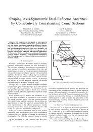
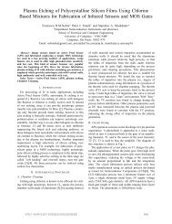
A. Internal RegionThe fields within the cavity are written as the sumof TE z and TM z components, with the aid of vectorpotential components Fz d and A d z, respectively. Each vectorpotential component is expressed in a double-Fourier seriesalready satisfying the boundary conditions at the wallsz = z 1c and z = z 2c :A d z(ρ,φ,z) =F d z (ρ,φ,z) =∞∑∞∑n=−∞ q=0n=−∞ q=0à ecz (ρ,n,q)e −jnφ[ ] qπcos (z − z 1c ) , (1)L zc∞∑ ∞∑˜F z es (ρ,n,q)e −jnφsin[ qπL zc(z − z 1c )], (2)Fig. 2.Example of feeding network with 6 probes.where L zc = (z 2c − z 1c ), the first superscript in Ãec z or˜F zes refers to an exponential Fourier series in φ, and thesecond superscript refers to a sine or cosine Fourier seriesin z.The vector potentials in spectral domain (Ãec z (ρ,n,q)esand ˜F z (ρ,n,q)) are a combination of Bessel functionsof order n. For an equivalent surface magnetic current¯M s (φ,z) = M φ (φ,z)â φ + M z (φ,z)â z at ρ = b, and afterimposing the boundary conditions at the metallic walls atρ = a and ρ = b, the potentials are given by:à ecz (ρ,n,q) =˜F z es (ρ,n,q) =˜GAdMφ(ρ,n,q)˜GFd˜Mecφ (n,q), (3)˜MecMφ(ρ,n,q) φ (n,q) +˜G Fd esMz(ρ,n,q) ˜M z (n,q), (4)Adwhere ˜GMφ(ρ,n,q) corresponds to the transform of theGreen’s function for the potential A d z(ρ,φ,z) due to a φ-directed magnetic surface current at ρ = b. And similarlyfor the other terms.B. External RegionThe external electromagnetic fields can be expanded inTE z and TM z components [14], with vector potentialsexpanded in cylindrical waves, satisfying the radiationcondition:A o z(ρ,φ,z) =F o z (ρ,φ,z) =∞∑n=−∞∞∑n=−∞∫ ∞−∞∫ ∞−∞à efz (ρ,n,k z )e −jkzz e −jnφ dk z(5)˜F efz (ρ,n,k z )e −jkzz e −jnφ dk zwhere the superscripts ef refer to an exponential series inφ and a Fourier transform in z, respectively. Imposing the(6)boundary conditions at the cylinder surface the potentialsare given by:à efz (ρ,n,k z ) =˜F z ef (ρ,n,k z ) =˜GAo˜GAoMφ(ρ,n,k z )˜GFo˜Mefφ (n,k z), (7)˜MefMφ(ρ,n,k z )φ (n,k z) +˜G FoefMz(ρ,n,k z ) ˜M z (n,k z ), (8)whereMφ(ρ,n,q) corresponds to the transform of theGreen’s function for the potential A o z(ρ,φ,z) due to a φ-directed magnetic surface current at ρ = b. And similarlyfor the other terms.C. FeedingThe wraparound antenna is fed by a parallel network atequally spaced N p coaxial cables along a circumference(z = z f , ρ = b) of the antenna. Each probe of the coaxialcables is modeled as a strip of width W f . An example ofthe feeding network, with 6 coaxial cables is shown in Fig.2. If the spacing between the feed points is smaller thanone wavelength in the dielectric substrate, the electric fieldis nearly uniform in φ, resulting a close to omnidirectionalpattern [15]. If each feed point carries a current I o , the totalcurrent in the network is N p I o .D. Method of MomentsThe boundary conditions at the dielectric-air interfacerequire the continuity of the tangential magnetic fields,which are obtained from the vector potentials (1-2) forthe internal region, and (7-8) for the external one. Theseconditions lead to integral equations solved by the methodof moments. The equivalence surface magnetic current is2009 SBMO/IEEE MTT-S International Microwave & Optoelectronics Conference (IMOC 2009) 58

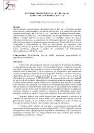
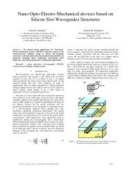
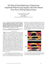
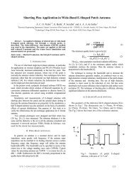
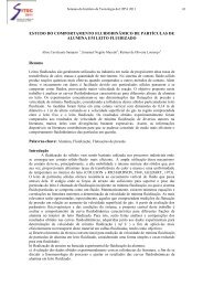
expanded in a set of basis functions:0M z (φ,z) =M φ (φ,z) =Umax∑u=−UmaxUmax∑u=−UmaxTzmax∑t=1Tφmax∑t=1M zut (φ,z) (9)M φut (φ,z) (10)60300.4300.80.6160The z-directed basis functions used (M zut (φ,z)) haveexponential variation in φ and rooftop in z, leading to apiecewise linear approximation in z. The φ-directed basisfunctions used (M φut (φ,z))have exponential variation inφ, but constant in z, leading to a piecewise constantapproximation in z. The integral equations are then testedby the same set of functions. Such procedure transformsthe integral equations in a set of linear equations, whichunknowns ([I]) are the coefficients of the basis functions:901201500.215012090[Z][I] = [V ] (11)180Once the equivalent surface magnetic current is known, theradiation pattern is obtained from far field approximationsof the fields at external region, followed by saddle-pointapproximation of radiation integrals [14]. And the inputimpedance is given by the stationary formula:∫ ∫1Z in = −(N p I o )∫V2 Ē( ¯M s ) · ¯J f dv (12)where J f is the total network current.III. RESULTSA comparison of the radiation pattern for the cavitybackedwraparound antenna, obtained with this formulation,and that of a microstrip wraparound antenna, obtainedwith cavity method [1],[3], is presented in Fig. 3. Thecylinder has radius of 26 mm, and a cavity of thicknessequal to 1 mm is filled with a dielectric of relativepermitivitty of 2.1. A wraparound antenna of 34.5 mm isprinted over the dielectric surface, and fed with 4 probesat z f = 8.625 mm, modeled as strips of 2 mm of width.It was observed that 4 probes were enough to radiate anomnidirectional pattern. The antenna is centered at a 50mm cavity, and evaluated at f = 3 GHz. Despite thedifferences in the geometry and methods of analysis, theradiation patterns show similar behavior.Figure 4 shows the input impedance of a wraparoundantenna of length L zc = 20 mm. The perfect cylindricalconductor has radius b = 21 mm, and the thickness ofthe cavity values (b − a) = 1 mm. It is filled with adielectric of relative permitivitty equal to 9.6. No dielectriclosses were considered. Four probes of coaxial cables wereused to reach an omnidirectional pattern. They were placedat z f = 5 mm, and modeled by a strip of width equalto 2 mm. The results were plotted around the frequencyFig. 3. Radiation pattern |E| × θ. ____ this formulation for acavity-backed wraparound antenna, - - - cavity method for a microstripwraparound antenna. f = 3 GHz, a = 25 mm, h = 1 mm, z 1c = −25mm, z 2c = 25 mm, z 1a = −17.25 mm, z 2a = 17.25 mm, z f =z.2a /2, W f = 2 mm, ε r=2.1, 4 probes at φ = 0, 90 o , 180 o , 270 o .2.3 GHz, which corresponds to the first omnidirectionalmode. Figure 4 also shows results from [10], for the casewhen there is no cavity, and the dielectric layer extendsto infinity in −z and +z-directions. The results from [10]were scaled by a factor of 7, as already shown in [4]. Theresults for the cavity-backed antenna of this formulationwere compared to those from a cylindrical microstrip one([10]) due to the lack of results for this specific geometry inthe literature. Despite the geometrical differences the inputimpedance of both geometries are very close. The cavityeffect can be observed in Fig. 5, where input impedancesare shown for cavities of 30 mm, 40 mm, and 50 mm. Asthe cavity size increases the effect of the perfect electricwalls at z = z 1c and z = z 2c diminishes. And nosignificant variation of the input resistance is observed forcavities of 40 mm or larger. But it also shows that for acavity of 40 mm there is a cavity resonance around 2.41GHz. Cavity design should avoid these resonances, thatcan endanger the impedance matching.IV. CONCLUSIONThis paper presented a method of moments solution fora cavity-backed cylindrical wraparound antenna. Resultsfor radiation pattern and input impedance were obtainedand compared to similar geometries in which the dielectricextends to infinity in z-direction. It was shown thatthe cavity-backed wraparound presents similar characteristicsas the microstrip one. The sensitivity of the input2009 SBMO/IEEE MTT-S International Microwave & Optoelectronics Conference (IMOC 2009) 59

(Ω)151050−5this formulation[10] microstrip wraparoundR inX in−102.1 2.15 2.2 2.25 2.3 2.35 2.4 2.45 2.5f (GHz)Fig. 4. Input impedance for a cavity-backed wraparound antenna. b =21 mm, a = 20 mm, z 1c = −25 mm, z 2c = 25 mm, z 1a = −10mm, z 2a = 10 mm, z f = 5 mm, W f = 2 mm, ε r=9.6, 4 probes atφ = 0, 90 o , 180 o , 270 o.1510R in[6] J. Ashkenazy, S. Shrikman, and D. Treeves, "Electric surface currentmodel for the analysis of microstrip antennas on cylindrical bodies",IEEE Trans. Antennas Propagat., vol. AP-33, pp. 295-300, Mar. 1985.[7] R. F. Harrington, Field Computation by Moment Method, New York:Macmillian, 1968.[8] L. C. Kempel, and J. L. Volakis, "Radiation by cavity-backedantennas on a circular cylinder", IEE Proceedings on Microwaves,Antennas and Propagation, vol. 142, No. 3, 1995, pp. 233-239.[9] S. M. Ali, T. M. Habashy, J. F. Kiang, and J. A. Kong, "Resonancein cylindrical-rectangular and wraparound structures", IEEE Trans.Microwave Theory Tech., vol. 37, No. 11, pp. 1773-1783, Nov. 1989.[10] T. M. Habashy, S. M. Ali, and J. A. Kong, "Input impedance and radiationpattern of cylindrical-rectangular and wraparound microstripantennas", IEEE Trans. Antennas and Propagat., vol. 38, No. 5, pp.722-731, May 1990.[11] F. C. Franklin, S. B. A. Fonseca, J. M. Soares, and A. J. Giarola,"Analysis of microstrip antennas on circular-cylindrical substrateswith a dielectric overlay", IEEE Trans. Antennas Propagat., vol. 39,No. 9, pp. 1398-1403, Sep. 1991.[12] C. C. Silva, Redes de antenas de microlinha moldadas sobre superfíciescilíndricas com interface optoeletrônica, PhD Thesis (inportuguese), Instituto Tecnológico da Aeronáutica, 1992.[13] O. M. C. Pereira Filho, "Flush-mounted Cylindrical-rectangularMicrostrip Antennas", IET Microwaves, Antennas & Propagation,Vol. 3, No. 1, pp. 1-13, 2009.[14] R. F. Harrington, Time-Harmonic Electromagnetic Fields, McGrawHill, 1961.[15] R. E Munson, "Conformal microstrip antennas and microstripphased arrays", IEEE Trans. Antennas and Propagation, vol. 22, pp.74-78, Jan. 1974.5(Ω)0−5X in−10L zc= 30 mmL zc= 40 mmL zc= 50 mm−152.1 2.15 2.2 2.25 2.3 2.35 2.4 2.45 2.5f (GHz)Fig. 5. Input impedance for a cavity-backed wraparound antenna. − −−L zc = 30 mm, ___L zc = 40 mm, ...L zc = 50 mm.impedance with the cavity size is also presented.REFERENCES[1] K-L. Wong, Design of Nonplanar Microstrip Antennas and TransmissionLines, Wiley Interscience, 1999.[2] C. C. Krowne, "Cylindrical-rectangular microstrip antennas", IEEETrans. Antennas Propagat., vol. AP-31, No. 1, pp. 194-199, Jan.1983.[3] C. Yang and Y. Z. Ruan, "Radiation Characteristics of WraparoundMicrostrip Antenna on Cylindrical Body", Electronic Letters, vol.29, No. 6, pp. 512-14.[4] K.-L. Wong and S.-Y. Ke, "Characteristics of the CylindricalWraparound Microstrip Patch Antenna", Proc. Natl. Sci. Counc.ROC(A), vol. 17, No. 6, pp438-42.[5] S. B. A. Fonseca and A. J. Giarola, "Analysis of MicrostripWraparound Antennas using Dyadic Green’s Functions", IEEETrans. Antennas and Propagation, vol. AP-31, No. 2, March 1983,pp. 248-53.2009 SBMO/IEEE MTT-S International Microwave & Optoelectronics Conference (IMOC 2009) 60