The Boundary Element Method for the Helmholtz Equation ... - FEI VÅ B

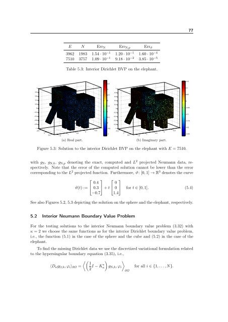
77E N Err N Err N,p Err ϑ3962 1983 1.54 · 10 −1 1.20 · 10 −1 1.60 · 10 −47510 3757 1.09 · 10 −1 9.18 · 10 −2 3.85 · 10 −5Table 5.3: Interior Dirichlet BVP on the elephant.3.50.151310.10.80.62.50.80.60.050.420.400.201.50.20−0.05−0.2−0.410.5−0.2−0.4−0.1−0.6−0.80−0.6−0.8−0.15−1−0.500.50.511.5(a) Real part.0−0.5−1−0.5−1−1−0.500.500.511.5(b) Imaginary part.−0.5−1−0.2−0.25Figure 5.3: Solution to the interior Dirichlet BVP on the elephant with E = 7510.with g N , g N,h , g N,p denoting the exact, computed and L 2 projected Neumann data, respectively.Note that the error of the computed solution cannot be lower than the errorcorresponding to the L 2 projected function. Furthermore, ϑ: [0, 1] → R 3 denotes the curve⎡ ⎤ ⎡ ⎤0.4 0ϑ(t) := ⎣ 0.3 ⎦ + t ⎣ 0 ⎦ for t ∈ [0, 1]. (5.4)−0.7 1.4See also Figures 5.2, 5.3 depicting the solution on the sphere and the elephant, respectively.5.2 Interior Neumann Boundary Value ProblemFor the testing solutions to the interior Neumann boundary value problem (3.32) withκ = 2 we choose the same functions as for the interior Dirichlet boundary value problem,i.e., the function (5.1) in the case of the sphere and the cube and (5.2) in the case of theelephant.To find the missing Dirichlet data we use the discretized variational formulation relatedto the hypersingular boundary equation (3.35), i.e.,⟨D κ g D,h , ϕ i ⟩ ∂Ω = 12 I − K∗ κg N,h , ϕ i∂Ωfor all i ∈ {1, . . . , N}.