The Boundary Element Method for the Helmholtz Equation ... - FEI VÅ B

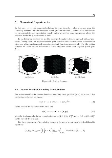
755 Numerical ExperimentsIn this part we provide numerical solutions to some boundary value problems using theboundary element method described in the previous sections. Although we concentrateon the computation of the missing Cauchy data, we provide some information about thesolution inside the given domain as well.In the following sections we use the Galerkin boundary element method with L 2 projectedCauchy data. We approximate the given Dirichlet and Neumann data by continuouspiecewise affine functions and piecewise constant functions, respectively. For the testingdomains we take a sphere, a cube and a rather simplified model of an elephant (see Figure5.1).110.80.80.60.610.40.20.40.20.80.60.4000.2−0.2−0.20−0.4−0.4−0.2−0.6−0.6−0.4−0.8−0.8−0.6−1−1−0.500.500.51 1(a) Sphere.−0.5−1−1−1−0.500.50.51 1(b) Cube.0−0.5−1−0.8−1−0.500.500.511.5(c) Elephant.−0.5−1Figure 5.1: Testing domains.5.1 Interior Dirichlet Boundary Value ProblemLet us first consider the interior Dirichlet boundary value problem (3.24) with κ = 2. Forthe testing solutions we choosein the case of the sphere and the cube andu(x) := (5i + 17x 1 )(11 + 7ix 2 )e iκx 3(5.1)u(x) := v κ (x, y 1 ) + v κ (x, y 2 ) (5.2)with the fundamental solution v κ and points y 1 := [1.2, 0.25, 0.7] T , y 2 := [1.2, −0.25, 0.7] Tin the case of the elephant.For the computation of the missing Neumann data g N,h we use the discretized Galerkinequations 1⟨V κ g N,h , ψ k ⟩ ∂Ω =2 I + K κ g D,h , ψ k for all k ∈ {1, . . . , E}∂Ω