The Boundary Element Method for the Helmholtz Equation ... - FEI VÅ B

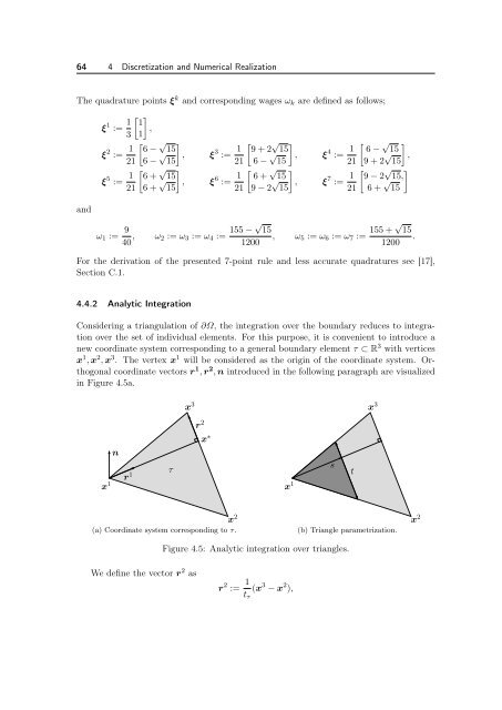
64 4 Discretization and Numerical RealizationThe quadrature points ξ k and corresponding wages ω k are defined as follows;and 11,ξ 1 := 1 3ξ 2 := 1 √ 6 − 1521 6 − √ , ξ 3 := 1 √9 + 2 151521 6 − √ 15ξ 5 := 1 √ 6 + 1521 6 + √ , ξ 6 := 1 √ 6 + 151521 9 − 2 √ 15ω 1 := 9 40 , ω 2 := ω 3 := ω 4 := 155 − √ 151200, ξ 4 := 121, ξ 7 := 121 √ 6 − 159 + 2 √ ,15 √ 9 − 2 15,6 + √ 15, ω 5 := ω 6 := ω 7 := 155 + √ 15.1200For the derivation of the presented 7-point rule and less accurate quadratures see [17],Section C.1.4.4.2 Analytic IntegrationConsidering a triangulation of ∂Ω, the integration over the boundary reduces to integrationover the set of individual elements. For this purpose, it is convenient to introduce anew coordinate system corresponding to a general boundary element τ ⊂ R 3 with verticesx 1 , x 2 , x 3 . The vertex x 1 will be considered as the origin of the coordinate system. Orthogonalcoordinate vectors r 1 , r 2 , n introduced in the following paragraph are visualizedin Figure 4.5a.x 3 r 2x 3nr 1τx ∗x 1 x 2sx 1 x 2t(a) Coordinate system corresponding to τ.(b) Triangle parametrization.Figure 4.5: Analytic integration over triangles.We define the vector r 2 asr 2 := 1 t τ(x 3 − x 2 ),