The Boundary Element Method for the Helmholtz Equation ... - FEI VÅ B

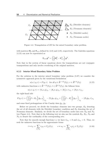
58 4 Discretization and Numerical RealizationΓ DE D (Dirichlet elements)E N (Neumann elements)Γ NN D (Dirichlet nodes)N N (Neumann nodes)Figure 4.4: Triangulation of ∂Ω for the mixed boundary value problem.with matrices M h and K κ,h defined by (4.8) and (4.9), respectively. The Galerkin equations(4.13) can now be represented as 1D κ,h g D =2 MT h − KT κ,h g N .Note that in the system of linear equations above the transpositions are not conjugatetranspositions and only involve reordering of the original matrices.4.3.3 Interior Mixed Boundary Value ProblemFor the solution to the interior mixed boundary value problem (3.37) we consider thesymmetric approach given by the variational formulationa(s, t, q, r) = F (q, r) for all q ∈ H −1/2 (Γ D ), r ∈ H 1/2 (Γ N ) (4.15)with unknown functions s ∈ H −1/2 (Γ D ), t ∈ H 1/2 (Γ N ), the bilinear formthe right-hand sideF (q, r) := 12 I + K κa(s, t, q, r) := ⟨V κ s, q⟩ ΓD − ⟨K κ t, q⟩ ΓD + ⟨K ∗ κs, r⟩ ΓN + ⟨D κ t, r⟩ ΓN , 1˜g D , q − ⟨V κ˜g N , q⟩ ΓD +Γ D2κI − K∗ ˜g N , r − ⟨D κ˜g D , r⟩ ΓNΓ Nand some fixed prolongations of the Cauchy data ˜g D , ˜g N .Before we proceed, we divide the boundary elements into two groups, E D denotingthe set of all elements with the Dirichlet boundary condition and E N denoting the set ofNeumann elements. Similarly, we divide the set of boundary nodes into sets N D and N N(see Figure 4.4). Note that in the following text we also use the symbols E D , E N , N D andN N to denote the cardinality of the corresponding sets.Note that for smooth enough functions t, s we have t| ΓD = 0 and s| ΓN = 0. Thus, weseek the unknown functions in the approximate formst ≈ t h := t i ϕ i ∈ T ϕ (Γ N ), s ≈ s h := s j ψ j ∈ T ψ (Γ D ) (4.16)i∈N N j∈E D