The Boundary Element Method for the Helmholtz Equation ... - FEI VÅ B

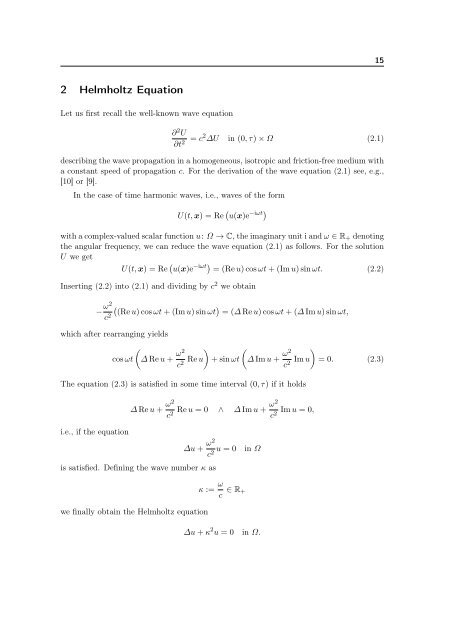
152 Helmholtz EquationLet us first recall the well-known wave equation∂ 2 U∂t 2 = c2 ∆U in (0, τ) × Ω (2.1)describing the wave propagation in a homogeneous, isotropic and friction-free medium witha constant speed of propagation c. For the derivation of the wave equation (2.1) see, e.g.,[10] or [9].In the case of time harmonic waves, i.e., waves of the formU(t, x) = Re u(x)e −iωtwith a complex-valued scalar function u: Ω → C, the imaginary unit i and ω ∈ R + denotingthe angular frequency, we can reduce the wave equation (2.1) as follows. For the solutionU we getU(t, x) = Re u(x)e −iωt = (Re u) cos ωt + (Im u) sin ωt. (2.2)Inserting (2.2) into (2.1) and dividing by c 2 we obtain− ω2c 2 (Re u) cos ωt + (Im u) sin ωt= (∆ Re u) cos ωt + (∆ Im u) sin ωt,which after rearranging yieldscos ωt∆ Re u + ω2c 2 Re u + sin ωt∆ Im u + ω2c 2 Im u = 0. (2.3)The equation (2.3) is satisfied in some time interval (0, τ) if it holdsi.e., if the equation∆ Re u + ω2ω2Re u = 0 ∧ ∆ Im u + Im u = 0,c2 c2 ∆u + ω2c 2 u = 0in Ωis satisfied. Defining the wave number κ asκ := ω c ∈ R +we finally obtain the Helmholtz equation∆u + κ 2 u = 0 in Ω.