Constitutive Equations

Constitutive EquationsDavid RoylanceDepartment of Materials Science and EngineeringMassachusetts Institute of TechnologyCambridge, MA 02139October 4, 2000IntroductionThe modules on kinematics (Module 8), equilibrium (Module 9), and tensor transformations(Module 10) contain concepts vital to Mechanics of Materials, but they do not provide insight onthe role of the material itself. The kinematic equations relate strains to displacement gradients,and the equilibrium equations relate stress to the applied tractions on loaded boundaries and alsogovern the relations among stress gradients within the material. In three dimensions there aresix kinematic equations and three equilibrum equations, for a total of nine. However, there arefifteen variables: three displacements, six strains, and six stresses. We need six more equations,and these are provided by the material’s consitutive relations: six expressions relating the stressesto the strains. These are a sort of mechanical equation of state, and describe how the materialis constituted mechanically.With these constitutive relations, the vital role of the material is reasserted: The elasticconstants that appear in this module are material properties, subject to control by processingand microstructural modification as outlined in Module 2. This is an important tool for theengineer, and points up the necessity of considering design of the material as well as with thematerial.Isotropic elastic materialsIn the general case of a linear relation between components of the strain and stress tensors, wemight propose a statement of the formɛ ij = S ijkl σ klwhere the S ijkl is a fourth-rank tensor. This constitutes a sequence of nine equations, since eachcomponent of ɛ ij is a linear combination of all the components of σ ij . For instance:ɛ 23 = S 2311 σ 11 + S 2312 σ 12 + ···+S 2333 ɛ 33Based on each of the indices of S ijkl taking on values from 1 to 3, we might expect a total of 81independent components in S. However, both ɛ ij and σ ij are symmetric, with six rather thannine independent components each. This reduces the number of S components to 36, as can beseen from a linear relation between the pseudovector forms of the strain and stress:1

⎧⎧ɛ x ⎡⎤ɛ yS 11 S 12 ··· S 16⎪⎨⎫⎪ɛ ⎬ zS 21 S 22 ··· S 26⎪⎨=γ ⎢. yz ⎣ . . .. ⎥ . ⎦γ xz ⎪⎩ ⎪ ⎭ S 61 S 26 ··· S 66 ⎪⎩γ xyσ xσ yσ zτ yzτxzτ xy⎫⎪ ⎬⎪ ⎭(1)It can be shown 1 that the S matrix in this form is also symmetric. It therefore it contains only21 independent elements, as can be seen by counting the elements in the upper right triangle ofthe matrix, including the diagonal elements (1 + 2 + 3 + 4 + 5 + 6 = 21).If the material exhibits symmetry in its elastic response, the number of independent elementsin the S matrix can be reduced still further. In the simplest case of an isotropic material, whosestiffnesses are the same in all directions, only two elements are independent. We have earliershown that in two dimensions the relations between strains and stresses in isotropic materialscan be written asɛ x = 1 E (σ x − νσ y )ɛ y = 1 E (σ y − νσ x )γ xy = 1 G τ xy(2)along with the relationEG =2(1 + ν)Extending this to three dimensions, the pseudovector-matrix form of Eqn. 1 for isotropic materialsis⎧⎪⎨⎪⎩ɛ xɛ y⎫⎪ɛ ⎬ z=γ yzγ xz ⎪ ⎭γ xy⎡⎢⎣1E−νE−νE−νE1E−νE−νE0 0 0−νE0 0 01E0 0 010 0 0G 0 010 0 0 0G 010 0 0 0 0G⎤⎧⎪⎨⎥⎦⎪⎩σ xσ yσ zτ yzτxzτ xy⎫⎪ ⎬⎪ ⎭(3)The quantity in brackets is called the compliance matrix of the material, denoted S or S ij . Itis important to grasp the physical significance of its various terms. Directly from the rules ofmatrix multiplication, the element in the i th row and j th column of S ij is the contribution of thej th stress to the i th strain. For instance the component in the 1,2 position is the contributionof the y-direction stress to the x-direction strain: multiplying σ y by 1/E gives the y-directionstrain generated by σ y , and then multiplying this by −ν gives the Poisson strain induced inthe x direction. The zero elements show the lack of coupling between the normal and shearingcomponents.The isotropic constitutive law can also be written using index notation as (see Prob. 1)ɛ ij = 1+νE σ ij − ν E δ ijσ kk (4)where here the indicial form of strain is used and G has been eliminated using G = E/2(1 + ν)The symbol δ ij is the Kroenecker delta, described in the Module on Matrix and Index Notation.1 G.M. Mase, Schaum’s Outline of Theory and Problems of Continuum Mechanics, McGraw-Hill, 1970.2

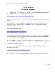
If we wish to write the stresses in terms of the strains, Eqns. 3 can be inverted. In cases ofplane stress (σ z = τ xz = τ yz = 0), this yields⎧⎪⎨⎪⎩σ xσ yτ xy⎫⎪⎬⎪ ⎭=⎡E ⎢1 − ν 2 ⎣1 ν 0ν 1 00 0 (1−ν)/2⎤⎧⎪⎨⎥⎦⎪⎩where again G has been replaced by E/2(1 + ν). Or, in abbreviated notation:where D = S −1 is the stiffness matrix.Hydrostatic and distortional componentsɛ xɛ yγ xy⎫⎪⎬⎪ ⎭(5)σ = Dɛ (6)Figure 1: Hydrostatic compression.A state of hydrostatic compression, depicted in Fig. 1, is one in which no shear stresses existand where all the normal stresses are equal to the hydrostatic pressure:σ x = σ y = σ z = −pwhere the minus sign indicates that compression is conventionally positive for pressure butnegative for stress. For this stress state it is obviously true that13 (σ x + σ y + σ z )= 1 3 σ kk = −pso that the hydrostatic pressure is the negative mean normal stress. This quantity is just onethird of the stress invariant I 1 , which is a reflection of hydrostatic pressure being the same inall directions, not varying with axis rotations.In many cases other than direct hydrostatic compression, it is still convenient to “dissociate”the hydrostatic (or “dilatational”) component from the stress tensor:σ ij = 1 3 σ kkδ ij +Σ ij (7)Here Σ ij is what is left over from σ ij after the hydrostatic component is subtracted. The Σ ijtensor can be shown to represent a state of pure shear, i.e. there exists an axis transformationsuch that all normal stresses vanish (see Prob. 5). The Σ ij is called the distortional, or deviatoric,3

where the factor 2 is needed because tensor descriptions of strain are half the classical strainsfor which values of G have been tabulated. Writing the constitutive equations in the form ofEqns. 8 and 9 produces a simple form without the coupling terms in the conventional E-ν form.Example 2Using the stress state of the previous example along with the elastic constants for steel (E = 207 GPa,ν =0.3,K = E/3(1 − 2ν) = 173 GPa,G = E/2(1 + ν) = 79.6 Gpa), the dilatational and distortionalcomponents of strain are⎡δ ij ɛ kk = δ ijσ kk3K= ⎣ 0.0289 0 0 ⎤0 0.0289 0 ⎦0 0 0.0289⎡⎤e ij = Σ 0 0.0378 0.0441ij2G = ⎣ 0.0378 0.0189 0.0567 ⎦0.0441 0.0567 −0.0189The total strain is then⎡ɛ ij = 1 3 ɛ kkδ ij + e ij = ⎣0.00960 0.0378 0.04410.0378 0.0285 0.05670.0441 0.0567 −0.00930If we evaluate the total strain using Eqn. 4, we have⎡ɛ ij = 1+νE σ ij − ν 0.00965 0.0377 0.0440E δ ijσ kk = ⎣ 0.0377 0.0285 0.05650.0440 0.0565 −0.00915These results are the same, differing only by roundoff error.⎤⎦⎤⎦Finite strain modelWhen deformations become large, geometrical as well as material nonlinearities can arise thatare important in many practical problems. In these cases the analyst must employ not only adifferent strain measure, such as the Lagrangian strain described in Module 8, but also differentstress measures (the “Second Piola-Kirchoff stress” replaces the Cauchy stress when Lagrangianstrain is used) and different stress-strain constitutive laws as well. A treatment of these formulationsis beyond the scope of these modules, but a simple nonlinear stress-strain modelfor rubbery materials will be outlined here to illustrate some aspects of finite strain analysis.The text by Bathe 2 provides a more extensive discussion of this area, including finite elementimplementations.In the case of small displacements, the strain ɛ x is given by the expression:ɛ x = 1 E [σ x − ν(σ y + σ z )]For the case of elastomers with ν =0.5, this can be rewritten in terms of the mean stressσ m =(σ x +σ y +σ z )/3as:2ɛ x = 3 E (σ x−σ m )2 K.-J. Bathe, Finite Element Procedures in Engineering Analysis, Prentice-Hall, 1982.5

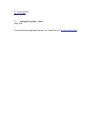
For the large-strain case, the following analogous stress-strain relation has been proposed:λ 2 x =1+2ɛ x= 3 E (σ x−σ ∗ m ) (10)where here ɛ x is the Lagrangian strain and σ ∗ m is a parameter not necessarily equal to σ m .The σ ∗ m parameter can be found for the case of uniaxial tension by considering the transversecontractions λ y = λ z :λ 2 y = 3 E (σ y − σ ∗ m)Since for rubber λ x λ y λ z =1,λ 2 y =1/λ x. Making this substitution and solving for σ ∗ m :Substituting this back into Eqn. 10,Solving for σ x ,σ ∗ m = −Eλ2 y3λ 2 x = 3 E= −E3λ x[σ x − E3λ x](λ 2 x − 1 λ x)σ x = E 3Here the stress σ x = F/A is the “true” stress based on the actual (contracted) cross-sectionalarea. The “engineering” stress σ e = F/A 0 based on the original area A 0 = Aλ x is:σ e = σ (x= G λ x − 1 )λ x λ 2 xwhere G = E/2(1 + ν) =E/3 forν=1/2. This result is the same as that obtained in Module2 by considering the force arising from the reduced entropy as molecular segments spanningcrosslink sites are extended. It appears here from a simple hypothesis of stress-strain response,using a suitable measure of finite strain.Anisotropic materialsFigure 3: An orthotropic material.If the material has a texture like wood or unidirectionally-reinforced fiber composites asshown in Fig. 3, the modulus E 1 in the fiber direction will typically be larger than those in thetransverse directions (E 2 and E 3 ). When E 1 ≠ E 2 ≠ E 3 , the material is said to be orthotropic.6

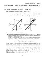
It is common, however, for the properties in the plane transverse to the fiber direction to beisotropic to a good approximation (E 2 = E 3 ); such a material is called transversely isotropic.The elastic constitutive laws must be modified to account for this anisotropy, and the followingform is an extension of Eqn. 3 for transversely isotropic materials:⎧⎪⎨⎪⎩ɛ 1ɛ 2γ 12⎫⎪⎬⎪ ⎭=⎡⎢⎣⎤1/E 1 −ν 21 /E 2 0⎥−ν 12 /E 1 1/E 2 0 ⎦0 0 1/G 12⎧⎪⎨⎪⎩σ 1σ 2τ 12⎫⎪⎬⎪ ⎭(11)The parameter ν 12 is the principal Poisson’s ratio; it is the ratio of the strain induced in the2-direction by a strain applied in the 1-direction. This parameter is not limited to values lessthan 0.5 as in isotropic materials. Conversely, ν 21 gives the strain induced in the 1-direction bya strain applied in the 2-direction. Since the 2-direction (transverse to the fibers) usually hasmuch less stiffness than the 1-direction, it should be clear that a given strain in the 1-directionwill usually develop a much larger strain in the 2-direction than will the same strain in the2-direction induce a strain in the 1-direction. Hence we will usually have ν 12 >ν 21 . There arefive constants in the above equation (E 1 , E 2 , ν 12 , ν 21 and G 12 ). However, only four of them areindependent; since the S matrix is symmetric, ν 21 /E 2 = ν 12 /E 1 .A table of elastic constants and other properties for widely used anisotropic materials canbe found in the Module on Composite Ply Properties.The simple form of Eqn. 11, with zeroes in the terms representing coupling between normaland shearing components, is obtained only when the axes are aligned along the principal materialdirections; i.e. along and transverse to the fiber axes. If the axes are oriented along some otherdirection, all terms of the compliance matrix will be populated, and the symmetry of the materialwill not be evident. If for instance the fiber direction is off-axis from the loading direction, thematerial will develop shear strain as the fibers try to orient along the loading direction as shownin Fig. 4. There will therefore be a coupling between a normal stress and a shearing strain,which never occurs in an isotropic material.Figure 4: Shear-normal coupling.The transformation law for compliance can be developed from the transformation laws forstrains and stresses, using the procedures described in Module 10 (Transformations). By successivetransformations, the pseudovector form for strain in an arbitrary x-y direction shown inFig. 5 is related to strain in the 1-2 (principal material) directions, then to the stresses in the 1-2directions, and finally to the stresses in the x-y directions. The final grouping of transformationmatrices relating the x-y strains to the x-y stresses is then the transformed compliance matrix7

Figure 5: Axis transformation for constitutive equations.in the x-y direction:⎧⎪⎨⎪⎩⎫ ⎧ɛ x ⎪⎬ ⎪⎨ɛ y = R⎪γ ⎭ ⎪ ⎩xy= RA −1 R −1 S⎫ ⎧ɛ x ⎪⎬ ⎪⎨ ɛ 1ɛ y12 γ ⎪⎭ = RA−1 ɛ⎪ 2 ⎩ 1xy2 γ 12⎧⎪⎨ σ 1⎪ ⎩⎫ ⎧⎪⎬ ⎪⎨σ 2 = RA −1 R −1 SA⎪τ ⎭ ⎪⎩12⎫⎧⎪⎬⎪⎨ ɛ 1⎪⎭ = RA−1 R −1 ɛ⎪ 2 ⎩⎫σ x ⎪⎬σ y ≡ S⎪τ ⎭ xy⎧⎪⎨⎪⎩γ 12⎫⎪⎬⎪ ⎭σ xσ yτ xy⎫⎪⎬⎪ ⎭where S is the transformed compliance matrix relative to x-y axes. Here A is the transformationmatrix, and R is the Reuter’s matrix defined in the Module on Tensor Transformations. Theinverse of S is D, the stiffness matrix relative to x-y axes:S = RA −1 R −1 SA, D = S −1 (12)Example 3Consider a ply of Kevlar-epoxy composite with a stiffnesses E 1 = 82, E 2 =4,G 12 =2.8(allGPa)andν 12 =0.25. The compliance matrix S in the 1-2 (material) direction is:⎡S = ⎣⎤ ⎡1/E 1 −ν 21 /E 2 0−ν 12 /E 1 1/E 2 0 ⎦ = ⎣0 0 1/G 12.1220 × 10 −10 −.3050 × 10 −11 0⎤−.3050 × 10 −11 .2500 × 10 −9 0 ⎦⎤2If the ply is oriented with the fiber direction (the “1” direction) at θ =30 ◦ from the x-y axes, theappropriate transformation matrix is⎡⎡.7500 .2500⎤.8660−sc sc c 2 − s 2 −.4330 .4330 .5000A = ⎣ c2 s 2 sc 2 2sc−2sc ⎦ = ⎣ .2500 .7500 −.8660 ⎦The compliance matrix relative to the x-y axes is then⎡S = RA −1 R −1 SA = ⎣ .8830 × ⎤10−10 −.1970 × 10 −10 −.1222 × 10 −9−.1971 × 10 −10 .2072 × 10 −9 −.8371 × 10 −10 ⎦−.1222 × 10 −9 −.8369 × 10 −10 −.2905 × 10 −9Note that this matrix is symmetric (to within numerical roundoff error), but that nonzero couplingvalues exist. A user not aware of the internal composition of the material would consider it completelyanisotropic.8

The apparent engineering constants that would be observed if the ply were tested in the x-y ratherthan 1-2 directions can be found directly from the trasnformed S matrix. For instance, the apparentelastic modulus in the x direction is E x =1/S 1,1 =1/(.8830 × 10 −10 )=11.33 GPa.Problems1. Expand the indicial forms of the governing equations for solid elasticity in three dimensions:equilibrium : σ ij,j =0kinematic : ɛ ij =(u i,j + u j,i )/2constitutive : ɛ ij = 1+νEσ ij − ν E δ ijσ kk + αδ ij ∆Twhere α is the coefficient of linear thermal expansion and ∆T is a temperature change.2. (a) Write out the compliance matrix S of Eqn. 3 for polycarbonate using data in theModule on Material Properties.(b) Use matrix inversion to obtain the stiffness matrix D.(c) Use matrix multiplication to obtain the stresses needed to induce the strains⎧⎪⎨ɛ =⎪⎩ɛ xɛ y⎫⎪ɛ ⎬ z=γ yzγ xz ⎪ ⎭γ xy⎧⎪⎨⎪⎩0.020.00.030.010.0250.03. (a) Write out the compliance matrix S of Eqn.3 for an aluminum alloy using data in theModule on Material Properties.(b) Use matrix inversion to obtan the stiffness matrix D.(c) Use matrix multiplication to obtain the stresses needed to induce the strains4. Given the stress tensor⎧⎪⎨ɛ =⎪⎩ɛ xɛ y⎫⎪ɛ ⎬ z=γ yzγ xz ⎪ ⎭γ xy⎧⎪⎨⎪⎩0.010.020.00.00.150.0⎫⎪⎬⎪⎭⎫⎪⎬⎪⎭σ ij =⎡⎢⎣1 2 32 4 53 5 7⎤⎥⎦(MPa)(a) Dissociate σ ij into deviatoric and dilatational parts Σ ij and (1/3)σ kk δ ij .9

(b) Given G = 357 MPa and K =1.67 GPa, obtain the deviatoric and dilatational straintensors e ij and (1/3)ɛ kk δ ij .(c) Add the deviatoric and dilatational strain components obtained above to obtain thetotal strain tensor ɛ ij .(d) Compute the strain tensor ɛ ij using the alternate form of the elastic constitutive lawfor isotropic elastic solids:ɛ ij = 1+νEσ ij − ν E δ ijσ kkCompare the result with that obtained in (c).5. Provide an argument that any stress matrix having a zero trace can be transformed to onehaving only zeroes on its diagonal; i.e. the deviatoric stress tensor Σ ij represents a stateof pure shear.6. Write out the x-y two-dimensional compliance matrix S and stiffness matrix D (Eqn. 12)for a single ply of graphite/epoxy composite with its fibers aligned along the x axes.7. Write out the x-y two-dimensional compliance matrix S and stiffness matrix D (Eqn. 12)for a single ply of graphite/epoxy composite with its fibers aligned 30 ◦ from the x axis.10