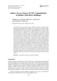
Table 2.Quick Reference Summary <strong>of</strong> Three Types <strong>of</strong> Attenuation <strong>Rate</strong> <strong>Constants</strong>Point Decay <strong>Rate</strong> Constant (k point ) Bulk Attenuation <strong>Rate</strong> Constant (k ) Biodegradation <strong>Rate</strong> Constant ( λ )USED FOR:Plume Duration Estimate. <strong>Use</strong>d toestimate time required to meet aremediation goal at a particular pointwithin the plume. If wells in the sourcezone are used to derive k point , then thisrate can be used to estimate the timerequired to meet remediation goals <strong>for</strong>the entire site. k point should not beused <strong>for</strong> representing biodegradation <strong>of</strong>dissolved constituents in ground-watermodels (use λ as described in the righth<strong>and</strong> column).Plume Trend Evaluation. Can be usedto project how far along a flow path aplume will exp<strong>and</strong>. This in<strong>for</strong>mation canbe used to select the sites <strong>for</strong> monitoringwells <strong>and</strong> plan long-term monitoringstrategies. Note that k should not beused to estimate how long the plume willpersist except in the unusual case wherethe source has been completelyremoved, as the source will keepreplenishing dissolved contaminants inthe plume.Plume Trend Evaluation. Can beused to indicate if a plume is stillexp<strong>and</strong>ing, or if the plume has reacheda dynamic steady state. <strong>First</strong> calculate λ,then enter λ into a fate <strong>and</strong> transportmodel <strong>and</strong> run the model to matchexisting data. Then increase thesimulation time in the model <strong>and</strong> see ifthe plume grows larger than the plumesimulated in the previous step. Notethat λ should not be used to estimatehow long the plume will persist except inthe unusual case where the source hasbeen completely removed.REPRESENTS:HOW TOCALCULATE:Nat. LogConcentrationMostly the change in source strengthover time with contributions from otherattenuation processes such asdispersion <strong>and</strong> biodegradation. k point isnot a biodegradation rate as itrepresents how quickly the source isAttenuation <strong>of</strong> dissolved constituents dueto all attenuation processes (primarilysorption, dispersion, <strong>and</strong> biodegradation).depleting. In the rare case where thesource has been completely removed(<strong>for</strong> a discussion <strong>of</strong> source zones, seeWiedemeier et al., 1999), k point willapproximate k .Plot natural log <strong>of</strong> concentration vs. Plot natural log <strong>of</strong> conc. vs. distance. Iftime <strong>for</strong> a single monitoring point <strong>and</strong> the data appear to be first-order,calculate k point = slope <strong>of</strong> the best-fit determine the slope <strong>of</strong> the natural logtrans<strong>for</strong>meddata by:line (ASTM, 1998). This calculationcan be repeated <strong>for</strong> multiple samplingpoints <strong>and</strong> <strong>for</strong> average plume1. Trans<strong>for</strong>ming the data by takingconcentration to indicate spatial trends natural logs <strong>and</strong> per<strong>for</strong>ming a linearin k point as well.regression on the trans<strong>for</strong>med data, orTimek point =Slope2. Plotting the data on a semi-log plot,taking the natural log <strong>of</strong> the y interceptminus the natural log <strong>of</strong> the x intercept<strong>and</strong> dividing by the distance between thetwo points.Multiply this slope by the contaminantvelocity (seepage velocity divided by theretardation factor R) to get k .The biodegradation rate <strong>of</strong> dissolvedconstituents once they have left thesource. It does not account <strong>for</strong>attenuation due to dispersion orsorption.Adjust contaminant concentration bycomparison to existing tracer (e.g.,chloride, tri-methyl benzenes) <strong>and</strong> thenuse method <strong>for</strong> bulk attenuation rate(see Wiedemeier et al., 1999); orCalibrate a ground-water solutetransport computer model that includesdispersion <strong>and</strong> retardation (e.g.,BIOSCREEN, BIOCHLOR, BIOPLUMEIII, MT3D) by adjusting λ; or<strong>Use</strong> the method <strong>of</strong> Buscheck <strong>and</strong>Alcantar (1995) (plume must be atsteady-state to apply this method).Notethis method is a hybrid between k <strong>and</strong> λas the Buscheck <strong>and</strong> Alcantar methodremoves the effects <strong>of</strong> longitudinaldispersion, but does not remove theeffects <strong>of</strong> transverse dispersion fromtheir λ.Note this calculation does not account<strong>for</strong> any changes in attenuationprocesses, particularly Dual-EquilibriumDesorption (availability) which canreduce the apparent attenuation rate atlower concentrations (e.g., see Kan etal., 1998).Nat. LogConcentrationSLOPE =k/ VgwDistance from SourceContam.Tracerλ = 0Find λλ6
Table 2.Continued...HOW TO USE:Point Decay <strong>Rate</strong> Constant (k point ) Bulk Attenuation <strong>Rate</strong> Constant (k) Biodegradation <strong>Rate</strong> Constant ( λ )To estimate plume lifetime:The time (t) to reach the remediationgoal at the point where K point wascalculated is:⎡ Cgoal ⎤− Ln ⎢ ⎥Cstartt =⎣ ⎦kpointTo estimate if a plume is showingrelatively little change:Pick a point in the plume butdowngradient <strong>of</strong> any source zones.Estimate the time needed to decay thesedissolved contaminants to meet aremediation goal as these contaminantsmove downgradient:⎡ Cgoal ⎤− Ln ⎢ ⎥Cstartt =⎣ ⎦kCalculate the distance L that thedissolved constituents will travel as theyare decaying using V s as the seepagevelocity <strong>and</strong> R is the retardation factor <strong>for</strong>the contaminant:To estimate if a plume is showingrelatively little change:Enter λ in a solute transport model thatis calibrated to existing plumeconditions. Increase the simulation time(e.g. by 100 years, or perhaps to theyear 2525), <strong>and</strong> determine if the modelshows that the plume is exp<strong>and</strong>ing,showing relatively little change, orshrinking.V sL = ⋅ tRIf the plume currently has not traveledthis distance L then this rate analysissuggests the plume may exp<strong>and</strong> to thatpoint. If the plume has extended beyondpoint L, then this rate analysis suggeststhe plume may shrink in the future. Notethat an alternative (<strong>and</strong> probably easiermethod) is to merely extrapolate theregression line to determine the distancewhere the regression line reaches theremediation goal.TYPICALVALUES:Reid <strong>and</strong> Reisinger (1999) indicated thatthe mean point decay rate constant <strong>for</strong>benzene from 49 gas station sites was0.46 per year (half-life <strong>of</strong> 1.5 years). ForMTBE they reported point decay rateconstants <strong>of</strong> 0.44 per year (half-life <strong>of</strong> 1.6years). In contrast, Peargin (2002)calculated rates from wells that werescreened in areas with residual NAPL;the mean decay rate <strong>for</strong> MTBE was 0.04per year (half life <strong>of</strong> 17 years) the rate <strong>for</strong>benzene was 0.14 per year (half life <strong>of</strong> 5years).For many BTEX plumes, k will be similarto biodegradation rates λ (on the order <strong>of</strong>0.001 to 0.01 per day; see Figure 5) asthe effects <strong>of</strong> dispersion <strong>and</strong> sorption willbe small compared to biodegradation.For BTEX compounds, 0.1 - 1 %/day(half-lives <strong>of</strong> 700 to 70 days)(Suarez <strong>and</strong>Rifai, 1999). Chlorinated solventbiodegradation rates may be lower thanBTEX biodegradation rates at somesites (Figures 5 <strong>and</strong> 6).Newell (personal communication)calculated the following median pointdecay rate constants: 0.33 per year (2.1year half-life) <strong>for</strong> 159 benzene plumes atservice station sites in Texas; <strong>and</strong> 0.15per year (4.7 year half-life) <strong>for</strong> 37 TCEplumes around the U.S.For more in<strong>for</strong>mation aboutbiodegradation rates <strong>for</strong> a variety <strong>of</strong>compounds, see Wiedemeier et al.,1999 <strong>and</strong> Suarez <strong>and</strong> Rifai, 1999.7