The cosmological evolution of galaxies and large scale structures ...

DOTTORATO DI RICERCA IN FISICAThe cosmological evolution of galaxiesand large scale structures frommulti-colour surveysTHESIS SUBMITTED TO OBTAIN THE DEGREE OF“Dottore di Ricerca” – Philosophiæ DoctorPHD IN PHYSICS – XXI CYCLE – OCTOBER 2008BYMarco CastellanoProgram CoordinatorProf. Enzo MarinariThesis AdvisorProf. Dario Trevese

To Giuliathe brightest star in my universe

ContentsContentsList of FiguresivxivIntroduction 11 Cosmological evolution of galaxies and structures 51.1 The Evolution of Galaxies . . . . . . . . . . . . . . . . . . . . . 51.1.1 Number Counts . . . . . . . . . . . . . . . . . . . . . . . 51.1.2 Luminosity Function . . . . . . . . . . . . . . . . . . . . 71.1.3 Mass Function . . . . . . . . . . . . . . . . . . . . . . . 111.1.4 Star Formation History . . . . . . . . . . . . . . . . . . . 121.1.5 Merging rates and disk size evolution . . . . . . . . . . . 151.1.6 Redshift evolution of AGN emission . . . . . . . . . . . . 161.2 Clusters of galaxies and their evolution . . . . . . . . . . . . . . . 171.2.1 General properties of cosmic structures . . . . . . . . . . 181.2.2 Observations of the intra-cluster plasma . . . . . . . . . . 251.2.3 Properties of cluster galaxies . . . . . . . . . . . . . . . . 281.3 Theoretical understanding of galaxy evolution . . . . . . . . . . . 341.3.1 Semianalytical models . . . . . . . . . . . . . . . . . . . 341.3.2 Environmental effects . . . . . . . . . . . . . . . . . . . 361.3.3 Origin of the red sequence . . . . . . . . . . . . . . . . . 402 The Observation of Structure Evolution 432.1 Multiwavelenght Surveys . . . . . . . . . . . . . . . . . . . . . . 432.1.1 Sky Surveys . . . . . . . . . . . . . . . . . . . . . . . . . 442.1.2 Deep Fields . . . . . . . . . . . . . . . . . . . . . . . . . 462.2 Photometric Redshifts . . . . . . . . . . . . . . . . . . . . . . . . 482.3 Cluster Detection Techniques . . . . . . . . . . . . . . . . . . . . 522.3.1 X-ray and SZ detections . . . . . . . . . . . . . . . . . . 532.3.2 Lensing detections . . . . . . . . . . . . . . . . . . . . . 542.3.3 Optical detections . . . . . . . . . . . . . . . . . . . . . . 552.3.4 Cluster detection using photometric redshifts . . . . . . . 59

ivCONTENTS3 A new Algorithm to Detect Clusters with Photo-z 633.1 The (2+1)D Algorithm: basic principles . . . . . . . . . . . . . . 643.2 Implementation of the Algorithm . . . . . . . . . . . . . . . . . . 663.3 Tests on Simulations . . . . . . . . . . . . . . . . . . . . . . . . 673.4 Comparison with other techniques . . . . . . . . . . . . . . . . . 734 Structures in the K20 Field 774.1 The K20 Photometric Catalogue . . . . . . . . . . . . . . . . . . 774.2 Density Evaluation . . . . . . . . . . . . . . . . . . . . . . . . . 784.3 Galaxy properties and environment . . . . . . . . . . . . . . . . . 814.4 Conclusions . . . . . . . . . . . . . . . . . . . . . . . . . . . . . 865 The Blue/Red Luminosity Function in the GOODS Field 895.1 The GOODS-MUSIC sample . . . . . . . . . . . . . . . . . . . . 895.2 Bimodality . . . . . . . . . . . . . . . . . . . . . . . . . . . . . 915.3 Luminosity Function . . . . . . . . . . . . . . . . . . . . . . . . 935.3.1 Non parametric Analysis . . . . . . . . . . . . . . . . . . 935.3.2 Parametric Analysis . . . . . . . . . . . . . . . . . . . . 945.3.3 B-band luminosity function for the total sample . . . . . . 955.3.4 Luminosity function for the blue/late and red/early galaxies 975.4 Environment of the red/early faint population . . . . . . . . . . . 1015.5 Conclusions . . . . . . . . . . . . . . . . . . . . . . . . . . . . . 1046 Structures in the GOODS Field 1076.1 A Photometrically detected Cluster at z ∼ 1.6 . . . . . . . . . . . 1076.1.1 Properties of the Structure . . . . . . . . . . . . . . . . . 1096.1.2 Spectroscopic confirmation . . . . . . . . . . . . . . . . . 1126.2 Large Scale Structures at 0.4 < z < 2.5 . . . . . . . . . . . . . . . 1136.2.1 Structures at z ∼ 0.7 . . . . . . . . . . . . . . . . . . . . 1186.2.2 Structures at z ∼ 1 . . . . . . . . . . . . . . . . . . . . . 1196.2.3 Structures at high z . . . . . . . . . . . . . . . . . . . . . 1216.2.4 Colour-Magnitude diagrams . . . . . . . . . . . . . . . . 1216.2.5 Galaxy properties as a function of the environment . . . . 1246.3 Conclusions and Discussion . . . . . . . . . . . . . . . . . . . . 127Conclusions 133Acknowledgments 139Publications 141Bibliography 143

List of Figures1.1 Original plot by Ryle & Scheuer (1955), showing the number ofradio sources in the second Cambridge (2C) survey versus theirflux in logarithmic scale. The dashed line corresponds to the slope-3/2 expected in an Euclidean universe. . . . . . . . . . . . . . . 61.2 Number-magnitude relations for various cosmological models inthe HST UBVI bands. The solid, dot-dashed, and dashed lines indicatestandard cold dark matter (Ω m = Ω 0 = 1, h = 0.5), openCDM (Ω m = Ω 0 = 0.3, h = 0.6), and Λ CDM (Ω m = 0.3,Ω Λ = 0.7, h = 0.7) cosmologies respectively (thick lines denotethe models including selection effects). The symbols indicate differentobservational datasets. Predictions from different modelsand data compilation are from Nagashima et al. (2002), see originalpaper for details. . . . . . . . . . . . . . . . . . . . . . . . . 81.3 Fig. 14 from the article by Jones et al. (2006). Comparison amongthe low redshift 6dFGS luminosity functions for K, J, rF, bJ bandsand those of other surveys. . . . . . . . . . . . . . . . . . . . . . 91.4 Fig 10 from Giallongo et al. (2005a): LF at intermediate and highredshift of late (left) and early (right) type galaxies separated followingtheir rest-frame colors according to a fit, with two Gaussiansprofiles, of their bimodal distribution. The LF in the lowestredshift bin 0.4 < z < 0.7 is also shown for comparison in allpanels (dotted curve). . . . . . . . . . . . . . . . . . . . . . . . . 101.5 Fig. 3 from the article by Pérez-González et al. (2008): localgalaxy stellar mass function estimated with the IRAC selected (filledstars), I-band selected (open stars), and MIPS selected (filled circles)samples at z < 0.2. The Schechter fit to the IRAC and I-banddata is shown with a solid black line, the best Schechter fit to thedata for the MIPS sample (i.e., for local star-forming galaxies) isplotted with a dashed line. Green asterisks and line show the MFfor H α -selected local star-forming galaxies. . . . . . . . . . . . . 12

viLIST OF FIGURES1.6 Fig. 4 from the article by Fontana et al. (2006): Galaxy stellarMass Functions in the GOODS-MUSIC sample, in different redshiftranges. Big circles represent the Galaxy Stellar Mass Functionsof the Ks-selected sample, computed with the 1/V max formalismup to the appropriate completeness level, as described inthe text, while small triangles show the Galaxy Stellar Mass Functionsof the Z 850 -selected sample. The dashed region represents thelocal GSMF of Cole et al. (2001). The solid line is the evolutionarySTY fit computed over the global redshift range 0.4 < z < 4 . . . . 131.7 Fig. 9 from the article by Elsner et al. (2008): Stellar mass densitiesas a function of redshift of their sample (filled circles) comparedwith values from literature. . . . . . . . . . . . . . . . . . . . . . 141.8 Fig. 1 from the article by Hopkins & Beacom (2006): Evolutionof SFR density with redshift from various datasets along with bestfittingparametric forms (solid lines). . . . . . . . . . . . . . . . . 141.9 Fig. 5 from the article by Ryan et al. (2008): Observed galaxymerger fraction from three different datasets plotted along with twodifferent parameterizations. . . . . . . . . . . . . . . . . . . . . . 151.10 Fig. 9 from the article by Trujillo et al. (2007): Size evolution ofthe most massive galaxies with look-back time: evolution with redshiftof the median ratio between the sizes of the galaxies in theirsample and the galaxies of the same stellar mass in the SDSS localcomparison sample is shown. Solid points indicate the size evolutionof spheroid-like galaxies. Open squares show the evolutionfor disc-like galaxies. . . . . . . . . . . . . . . . . . . . . . . . . 161.11 Fig. 9 from the article by Hopkins et al. (2007): Total numberdensity of quasars in various luminosity intervals (in log L/erg s −1 )as a function of redshift, from a best-fit evolving double power-lawmodel (lines) and a compilation of recent observations (symbols),in bolometric luminosity, B band, soft X-rays (0.5-2 keV), and hardX-rays (2-10 keV). The trend that the density of lower luminosityAGNs peaks at lower redshift is manifest in all bands. . . . . . . . 171.12 Two 4 ◦ slices, centred at declination −2.5 ◦ in the Northern GalacticPole, with 63381 galaxies from the 2dF redshift survey. Themaximum depth is z = 0.25 (Peacock et al. 2001) . . . . . . . . . 191.13 Fig. 6 from Meneux et al. (2008). (Left) Measurements of the projectedcorrelation function w p (r p ) of galaxies with different stellarmasses: log (M/M ⊙ ) ≥ 9.0 (open blue squares), ≥9.5 (filled redsquares), ≥10.0 (open green triangles) and ≥10.5 (filled magentatriangles) from VVDS data in the redshift range [0.5-1.2]. (Right)The best-fit parameters (r0 and γ) with their associated 1-, 2- and3σ error contours, derived from the variance among 40 mock catalogues.. . . . . . . . . . . . . . . . . . . . . . . . . . . . . . . 20

LIST OF FIGURESvii1.14 Fig. 5 from Sánchez & Cole (2008). Comparison of the powerspectra estimated from the full 2dFGRS and SDSS DR5 samples.The solid line shows the input power spectrum of the mock cataloguesused to estimate the covariance matrix of the measurements. 201.15 Fig. 10 from Lemze et al. (2008): 3D total mass profile for thecluster A1689. The profile derived in a model-independent way(dots) is compared to the one derived fitting an NFW profile ondata out to 693 h −1 kpc. Both profiles are shown with 1σ errors.The vertical line is at 0.1 r vir . . . . . . . . . . . . . . . . . . . . . 221.16 Fig. 6 from Barkana & Loeb (2001): mass of collapsing halos in aΛCDM cosmology. The solid curves show the mass of collapsinghalos which correspond to 1σ, 2σ, and 3σ fluctuations (in orderfrom bottom to top). The dashed curves show the mass correspondingto the minimum temperature required for efficient cooling withprimordial atomic species only (upper curve) or with the additionof molecular hydrogen (lower curve). . . . . . . . . . . . . . . . 241.17 Fig. 12 from Rosati et al. (2002). The sensitivity of the clustermass function to cosmological models. (Left) The cumulative massfunction at z = 0 for M > 5 × 10 14 h −1 M ⊙ for three cosmologies, asa function of σ 8 . Solid line, Ω m = 1; short-dashed line, Ω m = 0.3,Ω Λ = 0.7; long-dashed line, Ω m = 0.3, Ω Λ = 0. The shaded areaindicates the observational uncertainty in the determination of thelocal cluster space density. (Right) Evolution of n(> M, z) for thesame cosmologies and the same mass-limit, with σ 8 = 0.5 for theΩ m = 1 case and σ 8 = 0.8 for the low-density models. . . . . . . 251.18 Fig. 6 from Carlstrom et al. (2002): The cosmic microwave background(CMB) spectrum, undistorted (dashed line) and distortedby the Sunyaev-Zel’dovich effect (SZE) (solid line). To illustratethe effect, the SZE distortion shown is for a fictional cluster 1000times more massive than a typical massive galaxy cluster. The SZEcauses a decrease in the CMB intensity at frequencies 218 GHz andan increase at higher frequencies. . . . . . . . . . . . . . . . . . . 271.19 Fig. 4 from Dressler (1980): The fraction of E, S0 and S+I galaxiesas a function of the log of surface density. Also shown are anestimated scale of the real space density and the distribution ofthe total number of galaxies in bins of projected density (upperhistogram). . . . . . . . . . . . . . . . . . . . . . . . . . . . . . 28

viiiLIST OF FIGURES1.20 Fig. 1 from Balogh et al. (2004b): Filled circles in each panelshow the galaxy color distribution for the indicated 1 mag rangeof luminosity (right axis) and the range of local projected density,in units of Mpc −2 , shown on the top axis; 1σ error bars are givenby (N + 2) 1/2 , where N is the number of galaxies in each bin. Thesolid line is a double-Gaussian model, with the dispersion of eachdistribution a function of luminosity only. The reduced χ 2 value ofthe fit is shown in each panel. . . . . . . . . . . . . . . . . . . . . 291.21 Fig. 6 from Cooper et al. (2007): red fraction ( f R ) as a functionof redshift for galaxies in sliding bins of ∆z = 0.1. The highandlow-density samples (solid and dashed line respectively) areselected according to the extreme thirds of the local overdensitydistribution in the given z bin. The grey shaded regions give the1 − σ range of the red fractions in each density regime. . . . . . . 301.22 Fig. 7 from Cucciati et al. (2006). The fraction of the reddest ((u ∗ − g ′ ) ≥ 1.10, triangles) and bluest ( (u ∗ − g ′ ) ≤ 0.55, squares)galaxies is plotted as a function of the density contrast δ in differentredshift intervals (columns, as indicated on top) and for differentabsolute luminosity thresholds (rows, as indicated on the right).The shaded areas are obtained by smoothing the reddest(bluest)fraction with an adaptive sliding box containing the same numberof objects in each bin as the points marked explicitly. The numberof red and blue galaxies in each redshift and luminosity bin isexplicitly indicated in the corresponding panel. . . . . . . . . . . 311.23 Left: Fig. 1 from Bower et al. (1992b). Colour-Magnitude relationfor early type galaxies in the Coma (filled symbols) andVirgo (open symbols) clusters. Circles: elliptical galaxies: Triangles:S 0; Stars: S 0 a or S 0 3 . Solid lines show the median fit, thedashed line shows the relation expected in the Coma cluster fromthe zero point of the one in the Virgo cluster plus a distance moduluscorrection. Right: Fig. 15 from Demarco et al. (2007). ACScolor-magnitude diagram of spectroscopic (circles and triangles)and photometric members (squares) of the cluster RDCS J1252.9-2927 at z ∼ 1.24 along with the best fit color-magnitude relationand scatter from Blakeslee et al. (2003) shown in green. Note thatthe two plots use different photometries: once reported in the samebands and photometric system the C-M relations at low and highredshift have comparable slopes. . . . . . . . . . . . . . . . . . . 331.24 Fig. 8 from Mei et al. (2006): Colour Magnitude Relation absoluteslope δ(U − B) z /δB z and scatter σ(U − B) z for cluster ellipticals asa function of redshift. . . . . . . . . . . . . . . . . . . . . . . . . 34

LIST OF FIGURESix1.25 Fig. 10 from Treu et al. (2003): Regions of the cluster Cl 0024+16where key physical mechanisms are likely to operate. Top: Horizontallines indicate the radial region where the mechanisms aremost effective (in three-dimensional space). Bottom: For three projectedannuli the authors identify the mechanisms that could haveaffected the galaxy in the region (red). The blue numbers indicateprocesses that are marginally at work. The virial radius is 1.7 Mpc. 392.1 Fig. 2 from Reshetnikov (2005): characteristics of the main modernobservational projects. The horizontal dotted line shows thetotal area of the sky. The dashed curve shows the simplest observationalstrategy with F lim /S = const (F lim is the illumination fromthe faintest objects detected): such a dependence can be expectedif observations are carried out using one instrument with a fixedfield of view over a fixed total observation time. . . . . . . . . . . 442.2 Fig. 3 from Baum (1962): the mean SED for six elliptical galaxiesin the Virgo cluster (dashed curve) and for three similar galaxies inAbell 0801. . . . . . . . . . . . . . . . . . . . . . . . . . . . . . 492.3 Fig. 12 from Grazian et al. (2006a): Upper panel: the relation betweenthe spectroscopic (x-axis) and the photometric (y-axis) redshifton 668 galaxies with accurate spectroscopic redshift in theGOODS-MUSIC catalogue. In the inset, the distribution of the absolutescatter is shown and compared with a Gaussian distributionwith a standard deviation σ = 0.06 (smooth red curve). Lowerpanel: relative scatter restricted to the z < 2 range and discardingthe most discrepant objects in the same sample. . . . . . . . . . . 512.4 Fig. 4 from Rosati et al. (2002). Solid angles and flux limits of X-ray cluster surveys carried out over the past two decades. Darkfilled circles represent serendipitous surveys constructed from acollection of pointed observations. Light shaded circles representsurveys covering contiguous areas. . . . . . . . . . . . . . . . . . 543.1 Two examples of 3D FITS files showing the density field (left)and the selected clusters (right). The analyzed field is a simulationmimicking the GOODS field depth and survey area. The individuatedpeaks are clusters of M ∼ 10 14 M ⊙ at redshifts z ∼ 1 − 1.3 . . 683.2 Galaxies above an environmental density ρ 10 threshold 5 times theaverage, for redshifts 0.5, 1.0, 1.5 and 2.0 for catalogues with twodifferent limiting magnitudes. Filled dots represent real membersof the simulated richness class 0 clusters, while crosses representinterlopers. The contamination is reported in each panel. . . . . . 69

xLIST OF FIGURES4.1 Fig. 1 from Trevese et al. (2007): Photometric redshifts z phot versusspectroscopic redshifts z spec for all the galaxies in the cataloguewith spectroscopic observations (Grazian et al. 2006a, and refs.therein). Dashed lines indicate the r.m.s. uncertainty 0.05 · (1 + z). 784.2 Fig. 2 from Trevese et al. (2007): a) The distribution of photometricredshifts of the sample. b) Average ρ 10 density on the entirefield, in redshift bins, versus z as determined by the (2+1)Dalgorithm using for all sources: i) photometric redshifts (dashedline); ii) photometric redshifts, or spectroscopic redshifts wheneveravailable (continuous line). . . . . . . . . . . . . . . . . . . 794.3 Fig. 3 from Trevese et al. (2007): Isodensity contours of the surfacedensity Σ 10 as computed in the redshift slice 0.70 < z < 0.75,which includes the first detected structure (left panel). b) Sameplot for the second structure in the redshift slice 0.90 < z < 1.10(right panel). . . . . . . . . . . . . . . . . . . . . . . . . . . . . 794.4 Fig. 4 from Trevese et al. (2007): Galaxy colour distributions: athigh density (ρ 10 > 0.08Mpc −3 ) (shaded histogram), at low density(ρ 10 < 0.03Mpc −3 ), for the two structures at z∼0.70 (left) andz∼1.0 (right). . . . . . . . . . . . . . . . . . . . . . . . . . . . . 824.5 Fig. 5 from Trevese et al. (2007): Fraction of galaxies with restframe colour B-R>1.25 as a function of the volume density ρ 10 ,for the two structures at z∼0.70(left) and z∼1.0 (right). Error barsrepresent Poissonian fluctuation. . . . . . . . . . . . . . . . . . . 824.6 Fig. 6 from Trevese et al. (2007): Left panels: histograms of theC’ colour, defined in the text, for all the objects in the intervals0.7 < z < 0.8, 0.9 < z < 1.1, 1.4 < z < 1.7 (from the top).Dashed lines, corresponding to a local minimum, define the redand the blue populations. Right panels: rest-frame (U-V) vs. M Vdiagrams: the continuous line represents the fit to the points belongingto the red population, with a fixed slope α RS =0.08. Thedashed vertical line represents the reference absolute magnitudeM V = −20.7. The dotted line indicates the valley separating thetwo populations. . . . . . . . . . . . . . . . . . . . . . . . . . . 844.7 Fig. 7 from Trevese et al. (2007): The colour C ′ RS at M V rest=-20of the average red sequence, as computed from COMBO17 survey(circles), and resulting from the present analysis (triangles). Thestraight line represents a linear fit on all the data analysed in theCOMBO17 survey (adapted from Bell et al. 2004). . . . . . . . . 854.8 The slope of the rest-frame (U-B) vs. M B in the galaxy clusterscollected by Blakeslee et al. (2003) (open squares) and in the twostructures detected in the CDFS (filled squares). The dotted linerepresents the average value derived by Blakeslee et al. (2003). . 86

LIST OF FIGURESxi5.1 Total LF as a function of redshift. The continuous curves comefrom our maximum likelihood analysis. The point-line is the localLF (Norberg et al. 2002). The filled circles are the points obtainedwith 1/V MAX method. The empty circles come from the DEEP2survey (Willmer et al. 2006b). The results from the COMBO17and VDDS surveys are consistent with the DEEP2 results and areomitted in the plot. The dashed-point line is the model of Menciet al. (2006). . . . . . . . . . . . . . . . . . . . . . . . . . . . . . 965.2 LFs of the blue galaxies as function of redshift. The continuouscurves comes from our maximum likelihood analysis. The dottedlineis our fit at z ∼ 0.3, reported for comparison in all the redshiftbins. The big filled circles are the points obtained with 1/V MAXmethod. The little empty circle are points from the LFs by Willmeret al. (2006a). . . . . . . . . . . . . . . . . . . . . . . . . . . . . 985.3 LFs of the red galaxies as function of redshift. The continuouscurves comes from our maximum likelihood analysis, the first binof redshift, which have to low statistic, has been excluded from thisevolutive analysis. The dotted-line is our fit at z ∼ 0.5, reported forcomparison in all the redshift bins. The big filled circles are thepoints obtained with 1/V MAX method. The little empty circle arepoints from the LFs by Willmer et al. (2006a). The dashed-pointorange line is the model of Menci et al. (2006) . . . . . . . . . . . 995.4 LFs of the early type galaxies as function of redshift. The continuouscurves comes from our maximum likelihood analysis. Thedotted-line is our fit at z ∼ 0.5, reported for comparison in all theredshift bins. The big filled circles are the points obtained with1/V MAX method. . . . . . . . . . . . . . . . . . . . . . . . . . . 1005.5 panel a: Stellar mass distribution for the early and late population,the area of each histogram is normalised to unity. The arrows indicatethe mean value of the stellar mass for the early population(thin arrow) and for the late population (tick arrow) panel b: asthe panel a but for the distribution of ρ/ρ med panel c: Early typegalaxies vs. late type galaxies fraction as function of the densitycontrast (ρ/ρ med ). . . . . . . . . . . . . . . . . . . . . . . . . . . 1025.6 Surface density map in the redshift interval 0.4 < z < 0.6. Redregions are those of higher density (the white lines that surroundthem are those of density ∼ 2ρ = ρ med ), green regions are thosewith intermediate density (white lines ∼ ρ = ρ med ), dark blue regionsare the lower density ones (white lines ∼ ρ = 2ρ med ). . . . . 103

xiiLIST OF FIGURES6.1 Fig. 7 from Vanzella et al. (2006): Redshift distribution of thespectroscopic GOODS sample at z < 2. The signal has beensmoothed with a Gaussian filter with σ S = 300 km s −1 (the typicalerror in the redshift determination). The histogram has been obtainedcounting the number of sources in a window of 2000 km s −1moved from redshift 0 to 2 with a step of 100 km s −1 . The smoothedline is the “background” field distribution, obtained smoothing theobserved distribution with a Gaussian filter with σ S = 15 000 km s −1 .The peaks detected at S/N > 5 are marked with an arrow. . . . . . 1086.2 Density isosurfaces at z∼ 1.6 (average, average+1σ to average+6σ)superimposed on the z 850 band image of the GOODS-SOUTH field.The angular dimension of 1 Mpc (comoving) at z=1.6 is indicatedin the top-left corner. . . . . . . . . . . . . . . . . . . . . . . . . 1106.3 Histograms of the (U-V) color, total stellar mass (in solar units) andM B (AB) magnitude for objects selected in the field (shaded histogram)or in the cluster, as described in the text. In each panel weindicate the Kolmogorv-Smirnov probability of the null hypothesisthat the two samples are drawn from the same distribution. Theaverages of the distributions are indicated with arrows. . . . . . . 1116.4 Fraction of red galaxies, selected with (U-V) color, as described inthe text, on the entire GOODS field in the redshift interval 1.45

LIST OF FIGURESxiii6.8 Continuous line: redshift distribution of spectroscopically selectedAGNs in the GOODS-South field; dashed-line histogram is the distributionof the AGNs associated with overdensity peaks in Table6.1. Vertical lines are the positions of the detected structures. . . . 1156.9 Total mass of clusters at z ∼ 0.7 (top) and z ∼ 1.6 (bottom) fordifferent bias factors as a function of projected radius: bias=1(crosses) or bias=2 (filled sqaures). Each point is the average of themass computed according to equation 6.2 inside the range of projectedradius indicated by the horizontal errobar. The vertical errorbars represent the 3-sigma uncertainties on the computed mass.The ID is the identification number of Tab. 6.1. . . . . . . . . . . 1166.10 L X vs M 200 for the clusters in Tab 6.2. The horizontal error baris calculated considering a bias factor in the range 1 < b < 2,while the vertical error bars are computed varying the gas temperaturebetween T=1 keV and T=3 keV as discussed in the text. Theclusters at z ∼ 0.7 and z ∼ 1.6 are indicated by red points and errorbars. The M 200 − L X relations found by Reiprich & Böhringer(2002) and by Rykoff et al. (2008) are indicated by a black andgreen line respectively. . . . . . . . . . . . . . . . . . . . . . . . 1186.11 Galaxy isodensity levels at z ∼ 0.96 (black curves), as computedby our photo-z based code, plotted over the smoothed 0.5-2 keVChandra 2Ms image of the CDFS. The black cross marks the densitypeak. Blue circles are the cluster members; the green circle isthe extended source ID 183 in Luo et al. (2008) catalogue. . . . . 1206.12 Rest frame colour magnitude relations (U−B vs M B ) for each structureat z ∼ 0.7. Square are passively evolving galaxies selected asage/τ ≥ 4, and the circles are galaxies with age/τ < 4. Filledpoints indicate galaxies with spectroscopic redshift. The continuouslines are the fit to the red sequence of all the combined structure.The dotted lines constraint the error obtained with a jackknifeanalysis. . . . . . . . . . . . . . . . . . . . . . . . . . . . . . . . 1226.13 Same as Fig. 6.12. Panel a: structures at z ∼ 0.7; panel b: structuresat z ∼ 1; panel c: structure at z ∼ 1.6 ; panel d: structures atz ∼ 2.2. The dashed lines in the two last bins of redshift are the redsequence estimated at z ∼ 0.7 and ∼ 1 . . . . . . . . . . . . . . . 1236.14 Fraction of red (filled circles) and blue galaxies (filled triangles) fordifferent rest frame B magnitudes in four redshift intervals. Verticalerrorbars indicate the poissonian uncertainty in each bin. Theshaded areas are obtained by smoothing the red (blue) fraction withan adaptive sliding box. The horizontal errorbars indicate the rangeof density covered by the 5-95 % of the total sample. . . . . . . . 124

xivLIST OF FIGURES6.15 Galaxy stellar mass distribution in four redshift intervals. Shadedhistograms represent galaxies associated with the density peaksand empty histograms represent galaxies in the low density regions,as described in the text. In each panel the average value for the twodistributions are indicated by arrows. The K-S probability is reportedin each panel. . . . . . . . . . . . . . . . . . . . . . . . . 1266.16 As in Fig. 6.15 but for ages and SFRs of galaxies. . . . . . . . . . 127

IntroductionThe present-day universe arises because of a complex interaction between the microscopicaland macroscopical physical phenomena determining the evolution ofstars, galaxies and clusters of galaxies. Only in these last decades astrophysicistshave started to understand the complex physics involved in the evolution of galaxiesand of large scale structures in the universe. Particle and quantum physics inthe early universe, complex nuclear reactions, plasma physics and magnetohydrodynamicsin, and around, stars and condensed objects, as well as in the intergalacticmedium, are as important in shaping the observed universe as the gravitationalphysics determining the geometry and dynamics of single objects and of the universein general. To approach the underlying physical and cosmological problemsit is however necessary to solve first the astronomical problem of detecting andcharacterizing single galaxies and the larger structures containing them. To thisaim a great effort has been dedicated to develope, as a first step, techniques allowingto determine positions and redshifts of unbiased samples of thousands ofobjects, and then algorithms and routines allowing to reconstruct the large scalestructure of the universe traced by those galaxies.In this thesis we introduce a simple and physically grounded algorithm aimed atdetecting groups and clusters of galaxies exploiting deep multiwavelenght surveysin which galaxy redshifts are determined through broadband photometry (“photometricredshifts”) instead of spectroscopy. The use of photometric redshifts basedon a template fitting procedure allows, at the same time, to know with good accuracythe redshift of a galaxy, and to know some of its basic physical characteristics,like rest frame emission, mass and star formation rate. In addition, broadband photometrymakes possible to reach much fainter fluxes with respect to spectroscopicalobservations, thus pushing detection limits at the most distant observable objects.The algorithm presented in this thesis allows us to reconstruct the density fieldin the volume sampled by the photometric redshift survey, thus linking the galaxyproperties with the same space density influencing them, at an higher redshift withrespect to those investigated so far. Early collapse and formation of massive galaxiesby merging of smaller ones, tidal fields, dynamical or thermal interactions betweengalaxies and intra-cluster plasma, high speed galaxy encounters are all densitydependant phenomena thought to influence the observed environmental depen-

2 Introductiondence of galaxy properties. The study of the evolution of these properties at highredshift can give strong constraints on the physics of galaxy formation and evolution,while developing a reliable cluster detection technique designed for deepsurveys can be important also for future cosmological studies aimed at constrainingnow poorly investigated cosmological parameters, like the equation of state ofthe ’dark energy’, through the high redshift abundance and virialization status ofgroups and clusters.Some applications of the algorithm, aimed at characterizing the evolution ofthe environmental dependence of galaxy properties, are also presented. The maingoals of this application on deep multiwavelenght surveys of the Chandra DeepField South have been:• Detection both of known and of previously undetected structures as overdensitiesin the field, to provide confirmation of the ability of the algorithm inindividuating single high redshift clusters.• Analysis, whenever possible, of the basic properties of such groups/clusters:mass, richness, extension and density profile.• Cross-correlation of cluster positions with known extended (plasma halos)and point-like (AGNs) X-ray sources in the CDFS.• The study of the dependence, across cosmic time, of the fraction of ’earlytype’ galaxies, or “red fraction”, as a function of the environment: while thiskind of passively evolving galaxies are well known to populate present-dayclusters, it has not been well constrained when, and how, they start dominatingoverdense structures.• Study of the “red sequence” population: slope, colour and scatter of thelinear relation between colour and magnitude for early type galaxies cangive important constraints on the galaxy formation scenario.The thesis is organized as follows. In the first chapter we review the basicobservations characterizing the evolution of the average population of galaxiesand the present knowledge of the evolution of groups and clusters. At the end ofthe chapter we will summarize the present status in the theory of the evolution ofgalaxies and clusters: particular attention will be given to recent “semianalyticalmodels”, capable of explaining the evolutionary history of the universe with simpleyet physically meaningful recipes. In the second chapter we introduce some of themain tools employed so far in the study of the cosmic evolution: large surveys anddeep fields, the photometric redshift technique and cluster detection procedures,emphasizing recent developments in cluster detection with photometric redshifts.In the third chapter we give a description of the cluster detection algorithm presentedin this thesis along with tests on simulations and a qualitative comparisonwith other approaches. The fourth chapter is dedicated to the analysis of a deeppencil beam survey in a portion of the Chandra Deep Field South covering the area

Introduction 3of the K20 survey. Results on single clusters, on the variation of galaxy propertieswith environment and on the red sequence population will be presented. In the fifthchapter we present the photometric GOODS-MUSIC catalogue and the evolutionof the rest frame B-band luminosity function in the GOODS field, underlining theenvironmental properties of a population of faint red galaxies at intermidiate redshift.Finally, in the sixth chapter we present the analysis up to z ∼ 2.5 of theGOODS field and the resulting catalogue of groups and clusters. The propertiesof these structures and the environmental dependence of galaxy properties will beanalyzed in depth, putting particular attention to a forming cluster at z ∼ 1.6, oneof the highest redshifts structures ever detected. In the conclusions we will summarizethe results exposed in the present thesis along with perspectives on futuredevelopments of this research. The bibliography and a list of papers publishedduring the Ph.D. course can be found in the final pages of the thesis.

Chapter 1Cosmological evolution ofgalaxies and structuresThe field of cosmology and galaxy formation has made a huge progress over thepast 30-40 years: a great number of observations 1 made possible to investigatethe dynamics of the universe and its cosmological parameters and to establish thatgalaxies evolved through cosmic time. Some basic statistical quantities have shownthat the universe has undergone a complex history of formation of stars, galaxiesand large scale structures: number counts of galaxies and of X and radio sources;the history of star formation rate (SFR) in galaxies; the luminosity (LF) and massfunctions (MF) of galaxies, their merging rate and their size evolution and theevolution with redshift of active galactic nuclei (AGN) number density; correlationfunctions of different types of galaxies and larger structures (and their powerspectrum) as well as the evolution in number, galactic content and virializationstatus of groups and clusters of galaxies: while the first basic studies on numbercounts underlined that galaxies have evolved in the past Gyrs, the use of more complexstatistical tools, like luminosity and mass functions, allowed to individuate thephysical processes behind the evolutionary processes.1.1 The Evolution of Galaxies1.1.1 Number CountsEvidence for strong evolutionary changes in the properties of extragalactic objectswith cosmic time came from surveys of radio sources and quasars in the 1950sand 1960s. These studies showed an excess of faint sources as compared with theexpectations from uniform world models and steady state cosmologies (see Longair2006, and references therein). Deep counts of “normal” galaxies, which becameavailable in the 1980s and culminated in the observations of the Hubble Deep and1 In chap. 2 can be found a detailed description of wide surveys and deep fields from which mostof the results cited in the following paragraphs have been obtained

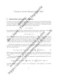
6 Cosmological evolution of galaxies and structuresUltra-Deep Field in recent years (e.g. Metcalfe et al. 1996), similarly showed anexcess of blue galaxies at faint magnitudes. Also the first X-ray surveys in the1990s presented the evidence for an excess of faint sources (e.g. Hasinger et al.1993). In a uniform, Euclidean universe the number N of galaxies as a function offlux S , or observed magnitude m, is given by the following expressions:N(≥ S ) ∝ S −3/2 (1.1)logN(≤ m) = 0.6m + constant (1.2)The first piece of evidence for an evolving comoving number density of extragalacticobjects came from the second Cambridge (2C) survey of radio sources,completed in 1954 by Ryle and collaborators (Ryle & Scheuer 1955) which founda huge excess of faint sources, the slope of the source counts between 20 and 60Jansky being described by N(≥ S ) ∝ S −3 (see Fig. 1.1). They concluded that theonly reasonable interpretation of these data was that the sources were extragalactic(similar to radio galaxy Cygnus A, discovered in 1946) and their comoving numberincreased at large distances. A better determination of the local luminosity functionof radio galaxies suggested a strong cosmological evolution in intrinsic luminosityas well as in comoving density. Intensive searches for radio-quiet quasars, throughFigure 1.1: Original plot by Ryle & Scheuer (1955), showing the number of radiosources in the second Cambridge (2C) survey versus their flux in logarithmic scale.The dashed line corresponds to the slope -3/2 expected in an Euclidean universe.

1.1 The Evolution of Galaxies 7their UV and IR excess emission with respect to normal stars, began in 1965 assoon as Sandage announced their discovery in that year (Sandage 1965). Since thefirst studies it was found considerable evidence that the number counts of opticallyselected quasars had slope steeper than 3/2 (as expected in an Euclidean universe)(Longair 2006). The first surveys adopting the identification of quasars throughmulticolour photometry showed a flattening of the integrated number counts ofradio-quiet quasars at z ≥ 2. By the early 1980s it was known that opticallyselected quasars exhibited strong cosmological evolution similar to that of radioquasars. It was later demonstrated that their number density has a maximum atredshifts z ∼ 2 − 3 and decline steeply at both lower and higher redshifts (see Sect.1.1.6).The birth of space astronomy expanded the wavelengths available to detect extragalacticobjects and brought definitive evidence for their overall evolution withcosmic epoch: the number counts of X-ray sources derived from observations madewith the ROSAT satellite (Hasinger et al. 1993) show that they follow the sametype of cosmological evolutionary behaviour as radio galaxies and quasars. Analogouslythe complete sky survey in the infrared bands (12.5 − 100µm) carried outby the IRAS satellite (Oliver et al. 1992) showed that there are more faint IRASsources than expected. Their emission, as well as the submillimeter emission ofthe sources detected by the ground-based SCUBA array, is originated by the lightemitted by dust heated at T ∼ 30 − 60K by the radiation coming from star formingregions. The abundance of faint sources at these wavelengths shows also that asignificative number of galaxies at high redshift were forming stars at rates higherthan those common in the present universe.Observations at optical wavelengths have shown, from the first surveys (e.g.Koo & Kron 1982) up to the deep fields observed by the Hubble Space Telescope(e.g. Metcalfe et al. 1996) and Subaru Deep Field (Nagashima et al. 2002), anexcess of faint objects (see Fig. 1.2). In the near infrared K band the counts followreasonably the expectations of uniform world models with a deceleration parameterq 0 ∼ 0 − 0.5 while at shorter wavelengths, and especially in the B band and inthe case of late and irregular morphological types, there is a large excess of faintgalaxies. Selection effects, K-corrections and the non-uniform spatial distributionare great obstacles in the determination of precise number counts. However, thanksto 8-meters class telescopes, CCD detectors and adaptive-optics mirrors developedin the last 15 years, wide and deep redshift surveys have been carried out allowingto determine accurate positions and magnitudes for thousands of galaxies and theirstatistical description through rest-frame luminosity functions.1.1.2 Luminosity FunctionWhile the study of number counts has demonstrated that the population of galaxieshas undergone a strong cosmological evolution, only the study of their rest-frameproperties and the evolution of their intrinsic luminosity distribution allows to determinewhether this is given by a pure density evolution, by a luminosity evolution

8 Cosmological evolution of galaxies and structuresFigure 1.2: Number-magnitude relations for various cosmological models in theHST UBVI bands. The solid, dot-dashed, and dashed lines indicate standard colddark matter (Ω m = Ω 0 = 1, h = 0.5), open CDM (Ω m = Ω 0 = 0.3, h = 0.6),and Λ CDM (Ω m = 0.3, Ω Λ = 0.7, h = 0.7) cosmologies respectively (thicklines denote the models including selection effects). The symbols indicate differentobservational datasets. Predictions from different models and data compilation arefrom Nagashima et al. (2002), see original paper for details.or by a combination of both. Since the first studies it was known that galaxies spana wide range of luminosities and it was attempted to analytically describe their distributionthrough simple functions. Many studies found that the galaxy LF can beparameterised with a Schechter shape (Schechter 1976):( L) αΦ(L) = φ ∗ L ∗ exp(− L )L ∗(1.3)where φ ∗ is the normalization factor, L ∗ is the luminosity cutoff between the exponentiallaw and the power-law shape, α is the slope of the power law. The advent oflarge surveys made possible the analysis of the luminosity function of the overallpopulation of galaxies as well as the LF of sub-samples of galaxies selected as afunction of their morphological, spectroscopic or colour properties. This permittedto probe the evolution of galaxies that have different star formation histories, quantifyingthis evolution also in terms of analytical parameters. Studies of the LF at

1.1 The Evolution of Galaxies 9Figure 1.3: Fig. 14 from the article by Jones et al. (2006). Comparison among thelow redshift 6dFGS luminosity functions for K, J, rF, bJ bands and those of othersurveys.different wavelengths help to discriminate the physical processes acting in differenttypes of galaxies and extragalactic environments. On the other hand, the analysisof the evolution of the LFs for different types of galaxies helps the comprehensionof the various star-formation histories.At low redshift the LFs of galaxies have been determined with great accuracymainly thanks to wide surveys like the Sloan Digital Sky Survey (SDSS York et al.2000), the 2dFGRS (Colless et al. 2001) and the 6dFRS (see Chap. 2). Consideringtogether all the populations of galaxies some remarkable differences are evidentfrom the analysis at different optical-NIR wavelengths (fig 1.3) in the low redshiftuniverse. First of all, the faint end slope of the LF tends to become steeper at bluerwavelengths because of an increased number of late type galaxies which are generallyfainter than early type ones. It appears also that the Schechter function may notbe a precise analytical description because of an upturn at faint magnitudes foundby several authors: for example Blanton et al. (2005b) adopt a double-schechterparametrisation to take in consideration the presence of an excess of low surfacebrightness blue galaxies with an exponential profile. Evidence has also been foundfor a rapid decline at very bright magnitudes (Jones et al. 2006). Numerous recentworks concentrated their attention on the LF of “red” and “blue” galaxies : i.e.objects selected according to the bimodal colour distribution that has been demonstratedto persist from low to high redshift (Strateva et al. 2001; Baldry et al. 2004;

10 Cosmological evolution of galaxies and structuresFigure 1.4: Fig 10 from Giallongo et al. (2005a): LF at intermediate and highredshift of late (left) and early (right) type galaxies separated following their restframecolors according to a fit, with two Gaussians profiles, of their bimodal distribution.The LF in the lowest redshift bin 0.4 < z < 0.7 is also shown forcomparison in all panels (dotted curve).Giallongo et al. 2005a). As we will see later, the separation into these two populationsarises spontaneously from the hierarchical process of galaxy formation andthe subsequent evolution which depends on the environment. Baldry et al. (2004)found that the red LF has a brighter characteristic luminosity and a shallower faintend slope with respect to the blue LF. These results have also been corroborated byBell et al. (2003). Differences have been found between the LF of galaxies in clustersand the LF of field and ’void’ galaxies (Popesso et al. 2005): the r-band LF inclusters shows a brighter exponential cutoff and a very steep low luminosity slope(that requires the LF to be analytically described by a double-Schechter function).The galaxy luminosity function has been studied at intermediate and high redshiftusing spectroscopic surveys like the DEEP2 (Willmer et al. 2006a) and theVVDS (Ilbert et al. 2005) or photometric surveys like the FORS Deep Field (Gabaschet al. 2004) and the COMBO17 (Bell et al. 2004) among others. They are less affectedby cosmic variance with respect to earlier studies but they still present somedifferences. However some general trends can be individuated: the total LF is dominatedby the blue/late type population that presents a faint end slope steeper thanthe red population and a fainter characteristic magnitude M ∗ (corresponding to theL ∗ in equation 1.1.2). The most evident trend is the brightening with redshift of M ∗ .The parameter φ ∗ is generally found to decrease with redshift but there are still uncertaintieson the magnitude of the density evolution. All the works found that the

1.1 The Evolution of Galaxies 11number density of red/early type galaxies has little evolution at z < 1. The analysisat intermediate and high redshift of the B band luminosity function by Giallongoet al. (2005a) found that both luminosity and density evolutions are needed to describethe cosmological behavior of the red/early and blue/late populations (Fig.1.4). The density evolution is greater for the early population with an increase by 1order of magnitude at z ∼ 0.4 with respect to the value at z ∼ 2 − 3. The luminositydensities of the early- and late-type bright galaxies appear to have a bifurcation atz ∼ 1. Indeed, while star-forming galaxies slightly decrease or keep constant theirluminosity density, “early“ galaxies increase in their luminosity density by a factorof 5-6 from z ∼ 2.5 − 3 to z ∼ 0.4 .1.1.3 Mass FunctionThe study of the Galaxy Stellar Mass Function (GSMF, or simply MF), that hasbeen the target of many studies in this last years, gives a detailed view on how theprocess of stellar assembly evolves as a function of the galaxy mass itself. To determinethe GSMF it is necessary to sample the optical and near infrared rest-frameemission of galaxies to reconstruct the spectral energy distribution (SED) at thiswavelengths. The stellar mass of the galaxy can be inferred from this observationsassuming stellar population synthesis (SPS) models adopting a universal initialmass function (IMF) for the stellar population. At low redshift, accurate GSMFhave been obtained from the 2dF (Cole et al. 2001) and 2MASS-SDSS (Bell et al.2003) surveys (Fig. 1.5), their results are in good agreement. The GSMF, as theluminosity function, can be analytically described by a Schechter function, at leastas a first approximation: in the local universe it has been found that the characteristicmass is larger for early type galaxies while the faint end slope is steeper forlate types. From this GSMF estimates of the stellar mass density of the universecan be derived.At high redshift the GSMF has been derived from the deep IR observations ofthe MUNICS, K20 and GOODS surveys. This last survey is based also on data inthe near and mid-infrared collected by the Spitzer satellite, which are fundamentalto estimate masses at very high redshift (Elsner et al. 2008). Since the first analysisit was evident a decline in the density of massive galaxies of the order of 50-70 %up to redshift ∼ 1. Fontana et al. (2006) found a mild decline of the more massivegalaxies, described by an exponential timescale of ∼6 Gyr, up to z ∼ 1.5, whilethe decline proceeds much faster thereafter, with an exponential timescale of ∼0.6 Gyr. Evidence has been found for a differential evolution of the GSMF, withlow mass galaxies evolving faster than more massive ones from z ∼ 1 - 1.5 to thepresent : the number of low mass galaxies at z∼ 1 is four times lower than the localone. However the slope of the low mass end of the GSMF remains close to thelocal one up to z ∼ 1 - 1.3 (Fig. 1.6). Pérez-González et al. (2008) found that 50%of the local stellar mass density was assembled at 0 < z < 1, and at least another40% at 1 < z < 4 with more massive galaxies assembled earlier than low massones: the bulk of their stellar content grew rapidly beyond z ∼ 3 in very intense

12 Cosmological evolution of galaxies and structuresFigure 1.5: Fig. 3 from the article by Pérez-González et al. (2008): local galaxystellar mass function estimated with the IRAC selected (filled stars), I-band selected(open stars), and MIPS selected (filled circles) samples at z < 0.2. TheSchechter fit to the IRAC and I-band data is shown with a solid black line, the bestSchechter fit to the data for the MIPS sample (i.e., for local star-forming galaxies)is plotted with a dashed line. Green asterisks and line show the MF for H α -selectedlocal star-forming galaxies.star formation events.The integral of the GSMF gives the total stellar mass density of the universeand allows the reconstruction of the building up of star populations in galaxies:comparing the outcome to the local value of Cole et al. (2001), Elsner et al. (2008)found that at least 42% of the stellar mass density was already in place at z = 1.This value decreases to 23% at z = 2 and about 7% at z = 3.5 (Fig. 1.7).1.1.4 Star Formation HistoryThere are various probes of on-going star formation rate (SFR) in galaxies: fora given population the various diagnostics can yield a global star formation rateρ S FR in units of M ⊙ yr −1 Mpc −3 . The cosmic star formation history (SFH), i.e.ρ S FR (z), displays, in a simple manner, the epoch and duration of galaxy growth.By integrating the function, one should recover the present stellar density. Eachdiagnostic has its advantages and drawbacks, furthermore, since star formationis often burst-like, one would not expect different diagnostics to give the samemeasure of the instantaneous SFR even for the same galaxies. Four methods have

1.1 The Evolution of Galaxies 13Figure 1.6: Fig. 4 from the article by Fontana et al. (2006): Galaxy stellar MassFunctions in the GOODS-MUSIC sample, in different redshift ranges. Big circlesrepresent the Galaxy Stellar Mass Functions of the Ks-selected sample, computedwith the 1/V max formalism up to the appropriate completeness level, as describedin the text, while small triangles show the Galaxy Stellar Mass Functions of theZ 850 -selected sample. The dashed region represents the local GSMF of Cole et al.(2001). The solid line is the evolutionary STY fit computed over the global redshiftrange 0.4 < z < 4been used in literature (Kennicutt 1998): rest-frame ultraviolet continuum, nebularemission lines, both directly caused by young star forming regions, the mid and farinfrared emission (10-300 µm) that arises from dust heated by young stars and radioemission (∼ 1.4GHz) thought to arise from synchrotron emission in the supernovaremnants following the rapid evolution of the most massive stars. Results based onUV observations depend on an assumed initial mass function and on the questionof whether dust extinction might be luminosity-dependent.First studies on the history of star formation across cosmic time were made byLilly et al. (1996), thanks to the Canada-France Redshift Survey, and by Madauet al. (1996) thanks to the Hubble Deep Field. Hopkins (2004) and Hopkins &Beacom (2006) have published a compilation of all recent results, standardizingall measures to the same initial mass function, cosmology and extinction law. Therecent results from the Sloan Digital Sky Survey, the Galaxy Evolution Explorer(GALEX) and the COMBO17 survey in the UV, and the Spitzer Space Telescopeat far-infrared wavelengths make it possible now to constrain the cosmic star formationhistory up to redshift z ∼ 1 (with a 30-50% uncertainty). Thanks to measurementsof the SFR at higher redshifts from the FIR, submillimeter, Balmer line

14 Cosmological evolution of galaxies and structuresFigure 1.7: Fig. 9 from the article by Elsner et al. (2008): Stellar mass densitiesas a function of redshift of their sample (filled circles) compared with values fromliterature.Figure 1.8: Fig. 1 from the article by Hopkins & Beacom (2006): Evolution ofSFR density with redshift from various datasets along with best-fitting parametricforms (solid lines).and UV emission, the cosmic star formation history is reasonably well determined(within a factor of ∼ 3 at z > 1) up to z ∼ 6 (Hopkins 2004; Hopkins & Beacom2006). In Fig 1.8, that summarizes their findings, some clear trends are evident: asystematic increase in star formation rate per unit volume out to z ∼ 1 (that can be

1.1 The Evolution of Galaxies 15fitted by the law: ρ S FR (z) ≈ (1 + z) 3.1 ) and a broad peak somewhere in the region2 < z < 4. The integration of the parameterized expression for the ρ S FR (z) yieldsa value of the present day mass density in remarkably good agreement with theone inferred from mass estimates (Cole et al. 2001). These results imply that mostof the star formation necessary to explain the presently- observed stellar mass hasalready been detected through various surveys. In addition this kind of studies allowus to predict fairly precisely the epoch by which time half of the present stellarmass was in place; this is z 1/2 = 2.0 ± 0.2.1.1.5 Merging rates and disk size evolutionThe redshift evolution of the galaxy merger fraction has been well studied up to z ∼2.5, counting pair of interacting objects or galaxies with disturbed morphologies.At z ≤ 1 the merger rate has been determined to be clearly evolving with redshift.It is roughly proportional to (1 + z) m , where typically 1 < m < 4. The broad rangeof values is likely due to different pair criteria, observational techniques, selectioneffects, and cosmic variance (Lin et al. 2008). Results obtained on the Hubble UltraDeep Field (HUDF) data show that the major merger fraction appears to peak atz ∼ 1.3 ± 0.4 (Ryan et al. 2008) implying that up to ∼ 40% of massive galaxieshave undergone a major merger since z ∼ 1 (Fig 1.9).Figure 1.9: Fig. 5 from the article by Ryan et al. (2008): Observed galaxy mergerfraction from three different datasets plotted along with two different parameterizations.Another approach to the assembly problem of galaxies is to explore the sizeevolution of massive systems at a given stellar mass. This is, however, a rathercomplicated observational issue: both masses and sizes can be derived only withgreat uncertainty and are influenced by many systematics and selection effects.The analysis by Trujillo et al. (2006a) on 10 massive galaxies in the interval 1.2

16 Cosmological evolution of galaxies and structuresFigure 1.10: Fig. 9 from the article by Trujillo et al. (2007): Size evolution of themost massive galaxies with look-back time: evolution with redshift of the medianratio between the sizes of the galaxies in their sample and the galaxies of the samestellar mass in the SDSS local comparison sample is shown. Solid points indicatethe size evolution of spheroid-like galaxies. Open squares show the evolution fordisc-like galaxies.size at a given stellar mass for low concentration objects was ∼ 2 times smaller atz ∼ 2.5. A comprehensive study by Trujillo et al. (2007) on DEEP2 data shows thatat a given stellar mass the evolution is particularly strong for more concentratedgalaxies, and that more massive galaxies evolve in size much faster than lowermass objects (particularly for disk-like galaxies) (see Fig. 1.10). All these resultsare in agreement with those obtained by Buitrago et al. (2008) on the GOODS field.They found that, at a given stellar mass, disk-like galaxies at z ∼ 2.3 were a factorof ∼ 2.6 smaller than present day equal mass systems, and spheroid-like galaxiesat the same redshifts were 4.3 times smaller than comparatively massive ellipticalgalaxies today. In turn, at higher redshifts (up to z ∼ 3), their results are compatiblewith a leveling off or a mild evolution in size.1.1.6 Redshift evolution of AGN emissionEnergetic emission, not attributed to stars, coming from the nuclei of galaxies, cannow be observed up to the highest redshifts, thanks to a variety of techniques: X-ray and radio emission, UV excess, emission lines and variability (Peterson 1997;Risaliti & Elvis 2004). All these observational techniques made possible to definedifferent classes of AGNs and to determine a unified scheme explaining their propertiesas determined by a central, massive, black hole accreting surrounding massat very high rates (Rees 1984; Antonucci 1993; Urry & Padovani 1995; Padovani

1.2 Clusters of galaxies and their evolution 171999). The finding that supermassive black holes are at the center of most nearbybright galaxies, and the observation of a very low space density of bright opticalquasars compared to galaxies, support the view of a very short active phase for supermassiveBHs which accrete surrounding gas. Deep observations (e.g. Fan et al.2001) have shown a significative redshift evolution of the quasar space density andof their luminosity function (QLF) in the rest-frame optical, soft and hard X-ray,and in the IR. It has been shown that the AGN space density grew through cosmictime reaching a peak and decreasing afterwards. The space density of low luminosityactive galactic nuclei peaks at redshifts lower than that of bright quasarsimplying a flattening of the QLF faint-end slope with redshift while the brightendslope of the QLF appears to become shallower toward higher redshifts (e.g.Hopkins et al. 2007, see Fig. 1.11).Figure 1.11: Fig. 9 from the article by Hopkins et al. (2007): Total number densityof quasars in various luminosity intervals (in log L/erg s −1 ) as a function of redshift,from a best-fit evolving double power-law model (lines) and a compilation ofrecent observations (symbols), in bolometric luminosity, B band, soft X-rays (0.5-2keV), and hard X-rays (2-10 keV). The trend that the density of lower luminosityAGNs peaks at lower redshift is manifest in all bands.1.2 Clusters of galaxies and their evolutionThe local Universe displays a rich pattern of galaxy clusters and superclusters whilethe early Universe was almost smooth, with only slight ripples seen in the cosmicmicrowave background radiation. The complex distribution of galaxies arised from

18 Cosmological evolution of galaxies and structuresthe homogeneous universe because of the effect of gravity: small initially overdensefluctuations attract additional mass as the Universe expands, and, at somepoint, the overdensities start to interact in non-linear ways creating the pattern ofpresent-day structures. Virialized overdensities (groups and clusters) present in thecomplex web of cosmic structures are the most massive relaxed objects in the universe.They have sizes of 1−3Mpc and are composed by hundreds or thousands ofgalaxies and by intra-cluster plasma whose characteristics can be studied throughtheir electromagnetic emission from the radio up to the gamma rays. The tendencyof galaxies to clusterize was noted from the earliest observations of the ’nebulae’but a systematic study of galaxy clusters started only with the first catalogues compiledby Abell (1958) and Zwicky & Rudnicki (1963). The first detections of theplasma emission in the X-rays were obtained in 1971 when the emission of the gasin the core of the Coma and Perseus clusters was detected. Radio observations ofclusters were first performed in early 1960’s while the Sunyaev-Zeldovich effect(compton scattering of CMB photons by the cluster plasma, Sunyaev & Zeldovich1972) was cleanly detected only starting in the 1980’s (Sarazin 1988). Clusterproperties evolve through cosmic time. We will mainly concentrate on the propertiesof cluster galaxies that, as in the case of the average galaxy population describedin the previous sections, evolve with time showing the evolutionary linkbetween environment and barionic matter.1.2.1 General properties of cosmic structuresStatistical description of the large scale structure of the universeThe complex 2D or 3D distribution of galaxies observed in large surveys (Fig.1.12) appears to be very irregular and ’sponge’-like. The statistical description ofthe distribution of galaxies and larger structures (statistically considered as points)is an important issue in cosmology and enable a better understanding of the natureand matter content of the universe as well as of its evolutionary history (Peebles1993).The distribution of galaxies can be studied using some basic statistical tools.The angular correlation function w(θ) representing the excess probability δP offinding a pair of galaxies separated by an angular separation θ (degrees) has beenthe first measure of clustering to be used on photographic plates (Longair 2006). Ina catalog averaging N galaxies per square degree, the probability of finding a pairseparated by θ can be written:δP = N(1 + w(θ))δΩ (1.4)where δΩ is the solid angle of the counting bin, (i.e. θ to θ + δθ). When theredshift of galaxies is measured, the radial distance can be calculated in the adoptedcosmology (Hogg 1999) and the corresponding spatial equivalent, ξ(r) in a catalogof mean density ρ (galaxies per Mpc 3 ) is thus:δP = ρ(1 + ξ(r))δr (1.5)

1.2 Clusters of galaxies and their evolution 19Figure 1.12: Two 4 ◦ slices, centred at declination −2.5 ◦ in the Northern GalacticPole, with 63381 galaxies from the 2dF redshift survey. The maximum depth isz = 0.25 (Peacock et al. 2001)w(θ) can be statistically linked to ξ(r) if the overall redshift distribution of thesources is available. Since the earliest studies it appeared evident that the distributionof galaxies is highly inhomogeneous. Indeed the correlation functions can berepresented by a power law:( ) −γ rξ(r) =(1.6)r 0where γ ∼ 1.8 both for the distribution of galaxies and of virialized clusters. Thequantity r 0 is the correlation length and it is an highly used measure of the degreeof clustering of different objects. It represents the distance at which ξ(r) = 1 andthus the probability of finding another object is two times the same probabilityfor a poissonian distribution (in which it is simply δP = ρ · δr) (Peebles 1993;Padmanabhan 1993). The observed clustering of galaxies is found to dependsignificantly on their specific properties, such as luminosity, color or spectral type,morphology and stellar mass both at low and high redshift. High luminosity, redand massive early type galaxies are generally found to be more clustered than bluelate type spirals. For example latest results obtained by the VIMOS survey showthat at z ∼ 1, the clustering length increases from r 0 ∼ 2.8h −1 Mpc for galaxies withmass M > 10 9 M ⊙ to r 0 ∼ 4.3h −1 Mpc when only the most massive (M > 10 10.5 M ⊙ )are considered. An increasing in the slope over the same range of masses is alsoobserved (Meneux et al. 2008) (Fig. 1.13).The power law behaviour of the correlation function is in agreement with thedistribution of galaxies being fractal up to a given scale: determining the scale atwhich a transition to the homogeneity observed in the CMB is reached has becomea key issue. An interesting debate on the validity of the assumptions behind theuse of the correlation functions (concerning finite size effects on the measure ofan average density and of its variance in an highly non-linear distribution) hasdeveloped in the last twenty years (e.g. Coleman & Pietronero 1992; Vasilyev et al.

20 Cosmological evolution of galaxies and structuresFigure 1.13: Fig. 6 from Meneux et al. (2008). (Left) Measurements of theprojected correlation function w p (r p ) of galaxies with different stellar masses:log (M/M ⊙ ) ≥ 9.0 (open blue squares), ≥9.5 (filled red squares), ≥10.0 (opengreen triangles) and ≥10.5 (filled magenta triangles) from VVDS data in the redshiftrange [0.5-1.2]. (Right) The best-fit parameters (r0 and γ) with their associated1-, 2- and 3σ error contours, derived from the variance among 40 mockcatalogues.Figure 1.14: Fig. 5 from Sánchez & Cole (2008). Comparison of the power spectraestimated from the full 2dFGRS and SDSS DR5 samples. The solid line showsthe input power spectrum of the mock catalogues used to estimate the covariancematrix of the measurements.

1.2 Clusters of galaxies and their evolution 212006; Sylos Labini et al. 2007, and refs. therein).With the development of wide surveys like the SDSS and the 2dFGRS thepower spectrum P(k) has become the preferred analysis tool because its form canbe readily predicted for various dark matter models. For a given density field ρ(x),the fluctuation over the mean is δ = ρ/¯ρ and the power spectrum in wavenumberspace is just the Fourier transform of the 3D correlation function:P(k) = 〈 ∫| δ 2 k |〉 = ξ(r)exp(i⃗k · ⃗r)d 3 r (1.7)The final power spectra for the completed 2dF and SDSS surveys are shownin Figure 1.14 (from Sánchez & Cole 2008): they partially disagree because the2dFGRS exhibits relatively more large-scale power than the SDSS, or, equivalently,SDSS has more small-scale power. Although these power spectra are generally ingood agreement with that predicted for a cold dark matter spectrum reproducingthe CMB angular fluctuations, more work is needed to understand the exact relationbetween the galaxy power spectrum and the linear perturbation theory predictionfor the power spectrum of matter fluctuations (Sánchez & Cole 2008).Dynamical properties of clustersIn the irregular distribution of galaxies visible in Fig. 1.12, groups and clusterslook like ’knots’ embedded inside a complex web of filaments and ’walls’ of galaxies.They are gravitationally bound and relaxed, or in a collapsing stage, and theycan cover a regular, almost spherical region of space, but they can as well havean ellipsoidal or more irregular shape. Indeed clusters can be represented as aone-dimensional sequence, running from regular to irregular clusters. Irregularclusters, often showing some degree of substructure, are considered systems in thephase of collapse and formation. On the other hand regular clusters have undergonea dynamical relaxation whose nature can be examined through the distributionof cluster galaxy velocities and positions. The Gaussian distribution has usuallybeen shown to be a consistent fit to the observed distribution function of velocitiesin many clusters (neglecting that the velocity dispersion generally decreases withdistance from the cluster center). While the Gaussian velocity distribution foundin clusters suggests that they are at least partially relaxed systems, they are notfully relaxed to a thermodynamic equilibrium in which all components of the clusterwould have equal temperatures; it is the velocity dispersion (not temperature)which is nearly independent of galaxy mass and position (Sarazin 1988). This kindof equilibrium configuration can be obtained by the process of ’violent relaxation’first described by Lynden-Bell (1967): a mixing of phase space occurs in the stronggravitational potential when the cluster forms, the fine grained phase space densityis preserved, but the coarse grained phase space density is mixed, yielding galaxyvelocities not dependent on the mass. Indeed classical two-body relaxation cannotoccur since it would require times longer than the Hubble time, while violentrelaxation has a much lower time scale of the order of the crossing time.

22 Cosmological evolution of galaxies and structuresThe typical velocity dispersions of galaxies in clusters are of the order of10 2 − 10 3 Km/s. Under the hypothesis of virial equilibrium they would correspondto gravitating masses in the range 10 14 − 10 15 M ⊙ . Through the observation of lensingeffects cluster total masses can be directly determined and then compared to themass inferred from optical or X-ray observations under the hypothesis of dynamicalequilibrium. A comparison of dynamical and lensing masses with the massof emitting stars (optical-IR) and plasma (X-rays) shows that only ∼ 15% of thegravitating mass is given by baryons, and that the gas mass is 5-6 times the massin stars and condensed objects. Thus the composition of a cluster of galaxies isroughly as follows: 80% of the mass is in dark matter; 17% in hot diffuse baryons;3% in the form of cooled barions, meaning stars or cold gas. The comparison of thedifferent distributions of the total matter (from weak lensing), of the hot gas (fromits X-ray emission), and of stars and cold gas (from galaxy density) in the clustermerger 1E 0657-558 (z=0.296), has recently led to an important empirical proofof the existence of dark matter in the form of weakly interacting massive particles(e.g. Clowe et al. 2006).Figure 1.15: Fig. 10 from Lemze et al. (2008): 3D total mass profile for the clusterA1689. The profile derived in a model-independent way (dots) is compared to theone derived fitting an NFW profile on data out to 693 h −1 kpc. Both profiles areshown with 1σ errors. The vertical line is at 0.1 r vir .From the point of view of the spatial distribution of galaxies a number of modelshave been proposed. Among the simplest are the isothermal models, whichassume a radial velocity distribution for galaxies that is Gaussian, isotropic andindependent of position. Considering that the galaxy distribution is stationary, thatgalaxy positions are uncorrelated and that the cluster is a collisionless system, aspatial distribution equivalent to that of an isothermal gas sphere in hydrostaticequilibrium is recovered. However in this simple model, at large radii, the totalnumber of galaxies and total mass diverge, thus some truncated models have been

1.2 Clusters of galaxies and their evolution 23proposed. The following is an analytic function which is a reasonable approximationto the inner portions of an isothermal truncated distribution (King 1962):ρ(r) = ρ 0 [1 + ( r r c) 2 ] −3/2 (1.8)in which ρ 0 is the central density and r c is the core radius. Galaxy spatial distributioncan be influenced also by dynamical friction properties, expecially in thecluster cores, while the underlying dark matter distribution is shaped only by theprocess of gravitational collapse. Numerical N-body simulations of the formationof cold dark matter halos have shown that the equilibrium density profiles of CDMhalos of all masses can be accurately fitted by the simple formula (Navarro et al.1997):δ cρ(r) = ρ crit ·( r r s)(1 + r r c) 2 (1.9)in which ρ crit is the critical density of the universe, r s is a scale radius and δ c isa characteristic (dimensionless) density. Gravitational lensing has shown that theNFW formula is in very good agreement with observed dark matter profiles (e.g.Lemze et al. 2008), see Fig. 1.15.Cluster mass functionGroups and clusters of galaxies are the largest structures to arise from the evolutionof the initial density fluctuations. The linear theory of evolution of the initialfield of density fluctuations and a simple schematization of the virialization processmake possible to analytically compute the distribution of masses of these virializedstructures once the initial conditions and cosmological parameters are known(Peebles 1993; Padmanabhan 1993). A simple yet accurate formula that gives thenumber density N(M) of virialized halos in the range M, M+dM is the one derivedby Press & Schechter (1974):N(M)dM =√2πρMδ c (z)σ 2dσdM exp(−δ c(z) 2)dM (1.10)2σ2 where δ c (z) is the overdensity threshold above which the structure decouples fromthe rest of the expanding universe and start to collapse and σ(M) is the mass varianceof density fluctuations. While σ(M) depends only on the initial conditions(normalization and shape of the power spectrum of the density field), δ c (z) dependson the cosmological parameters describing the dynamics of the universe:the total density parameter Ω 0 , the density parameter of the cosmological constantor dark energy Ω Λ and the parameter w of the dark energy equation of state.Recent observations confine the standard set of cosmological parameters to a relativelynarrow range centered on the following values: Ω m = 0.3, Ω Λ = 0.7,Ω b = 0.045, σ 8 = 0.9, a primordial power spectrum index n = 1 and a Hubbleconstant H 0 = 70km s −1 Mpc −1 . In such a universe dominated by cold dark matterand by a cosmological constant, progressively larger are halos represent the typical

24 Cosmological evolution of galaxies and structuresfluctuations to collapse at different cosmic times: as shown in Fig. 1.16, while atz ∼ 10 the halo mass which correspond to a 3σ fluctuation is 4.8×10 9 M ⊙ , at z ∼ 5,3σ collapsing halos have masses of 7.0 × 10 11 M ⊙ and in the present universe thetypical collapsing masses correspond to structures like cluster of galaxies (Loebet al. 2008). Thus the mass function changes across time: its dependence on cosmologyallows to put important experimental constraints on cosmological parametersfrom the observation of the redshift evolution of the cluster mass function (e.g.Voit 2005; Tozzi 2007, see Fig. 1.17). Many numerical simulations support thevalidity of the PS approach even if some discrepancies have been found that can bedescribed by more complicated fitting formulae (Jenkins et al. 2001). In additionthe PS formalism can be extended to give some statistical quantities that provedto be very useful in interpreting observational data: complete merger histories ofsingle halos (Lacey & Cole 1994), conditional probability function of progenitorhalos (Bower 1991) and the biased distribution of halos within halos (Mo & White1996).Figure 1.16: Fig. 6 from Barkana & Loeb (2001): mass of collapsing halos ina ΛCDM cosmology. The solid curves show the mass of collapsing halos whichcorrespond to 1σ, 2σ, and 3σ fluctuations (in order from bottom to top). Thedashed curves show the mass corresponding to the minimum temperature requiredfor efficient cooling with primordial atomic species only (upper curve) or with theaddition of molecular hydrogen (lower curve).

1.2 Clusters of galaxies and their evolution 25Figure 1.17: Fig. 12 from Rosati et al. (2002). The sensitivity of the cluster massfunction to cosmological models. (Left) The cumulative mass function at z = 0for M > 5 × 10 14 h −1 M ⊙ for three cosmologies, as a function of σ 8 . Solid line,Ω m = 1; short-dashed line, Ω m = 0.3, Ω Λ = 0.7; long-dashed line, Ω m = 0.3, Ω Λ= 0. The shaded area indicates the observational uncertainty in the determinationof the local cluster space density. (Right) Evolution of n(> M, z) for the samecosmologies and the same mass-limit, with σ 8 = 0.5 for the Ω m = 1 case and σ 8 =0.8 for the low-density models.1.2.2 Observations of the intra-cluster plasmaClusters appear as strong-contrast sources in the X-ray sky thanks to the emissionby an optically thin plasma that permeates the intra-cluster space. The continuumemission from a hot diffuse plasma is due primarily to three processes, thermalbremsstrahlung (free-free emission), recombination (free-bound) emission, andtwo-photon decay of metastable levels but, thanks to the high temperatures causedby the infalling of the gas in the deep cluster potential wells, the main continuumemission process is the bremsstrahlung (Sarazin 1988).Given the short timescales for elastic Coulomb collisions between particles,the plasma is in collisional equilibrium, therefore its typical temperature is set bythe large dynamical masses of clusters (10 14 − 10 15 M ⊙ ) to be in the range of 10-100 millions K (corresponding to an energy in the range 1-10 keV). Because ofthese high temperatures most of the emission is in the X-ray band. The total X-rayemission due to thermal bremsstrahlung is obtained by integrating the emissivityof a single charged particle over the distribution of speeds of the plasma electrons,over the frequencies and over the cluster volume :L X = 4.2 · 10 44( T ) 1/2 n 0 r c(6keV 2 · 10 −3 cm −3 )2 (0.25Mpc )2 erg/s (1.11)Another contribution to the X-ray luminosity comes from the line emission dueto heavy ions. This contribution is generally negligible in terms of total emissionbut it is important when studying the production of metals in cluster galaxies andtheir diffusion into the ICM (Tozzi 2007). Assuming clusters to be isothermal

26 Cosmological evolution of galaxies and structuresand in hydrostatic equilibrium, but allowing the gas to have a different velocitydispersion with respect to the galaxies, the gas density profile within the potentialwell associated with a King dark-matter density profile is well described by theβ-model (Cavaliere & Fusco-Femiano 1976):ρ(r) = ρ 0 [1 + ( r r c) 2 ] −3β/2 (1.12)The parameter β = µm pσ 2 rK B Tis the ratio between kinetic dark-matter energy (µ isthe mean molecular weight in mass units and σ r is the one-dimensional velocitydispersion) and thermal gas energy. If the thermodynamic of the ICM is entirelydetermined by gravitational processes, such as adiabatic compression during thecollapse and shocks due to supersonic accretion, as long as there are no preferredscales both in the cosmological and in the physical framework, clusters of differentmasses are just a scaled version of each other and obey simple scaling relations.However observations show that other processes like feedback from a non gravitationalastrophysical source (“preheating”) or the effects of inhomogeneities ormagnetic fields, break the scaling relations increasing the entropy of the ICM andthus lowering the X-ray luminosities, mainly in small clusters. In addition it iswell known that clusters are not perfectly isothermal, showing a mild decrease ofT outwards and, in nearly half of the local clusters, a significative drop in the innerregions (“cool cores”) (Rosati et al. 2002). With the knowledge of the T profile,a polytropic law can be used in the equation of hydrostatic equilibrium to determinethe density profile and the total gas mass with more accuracy. In many cases,however, the assumption of isothermality is a good approximation and enables todetermine the physical characteristics of clusters to be used when computing massfunctions and gas fractions for cosmological purposes.An important effect related to the presence of the thin intra-cluster plasma is theCompton scattering of the CMB photons on the free electrons of the ICM, known asSunyaev-Zeldovich effect (Sunyaev & Zeldovich 1972; Rephaeli 1995). Scatteringoff the moving electrons causes Doppler frequency shifts, and as the electron gasis very hot, photons gain energy. Conservation of photon number in the scatteringimplies that there is a systematic shifts of photons from the Rayleigh-Jeans to theWien side of the spectrum. The change of spectral intensity of the CMB radiationalong the line of sight of the cluster, in the non-relativistic limit, is:∆I = i 0 yg(x) (1.13)where: i 0 = 2(KT 0 ) 3 /(hc) 2 , (T 0 is the black-body temperature of the CMB spectrum,x = hν/KT). g(x), which defines the spectral form of the effect, is a functionwhich is zero at ν = 217GHz (Fig. 1.18). The spatial dependence of the effect iscontained in the comptonization parameter y given by the following integral alongthe line of sight:∫ ( KT)y =mc 2 n e σ t dl (1.14)

1.2 Clusters of galaxies and their evolution 27Figure 1.18: Fig. 6 from Carlstrom et al. (2002): The cosmic microwave background(CMB) spectrum, undistorted (dashed line) and distorted by the Sunyaev-Zel’dovich effect (SZE) (solid line). To illustrate the effect, the SZE distortionshown is for a fictional cluster 1000 times more massive than a typical massivegalaxy cluster. The SZE causes a decrease in the CMB intensity at frequencies 218GHz and an increase at higher frequencies.where n e is the electron density and σ t is the Thomson cross section. y can alsobe used as a measure of cluster mass being a measure of the total thermal energyof the electrons, proportional to the total gas mass (Voit 2005). When additionalkinematic effects and relativistic corrections, as long as possible contaminationsources, are taken in consideration, the SZ effect is probably the most powerfultool to compute a direct measurement of the evolution of the number density ofgalaxy clusters (Carlstrom et al. 2002): in fact SZ observations are particularlywell suited for deep surveys because they are able to detect all clusters above amass limit, independently of the cluster redshift. Indeed the SZ effect, as a distortionof the cosmic microwave background spectrum, does not suffer cosmologicaldimming with redshift. Once the redshift of the cluster is known, combining X-rayand SZ observations a direct measure of the Hubble constant can also be obtainedexploiting the different density dependencies of the SZ effect and X-ray emission(Cavaliere et al. 1979). The SZ effect is proportional to the first power of the electrondensity n e while the X-ray emission is proportional to the second power of n e ,so the angular diameter distance, that is a function of the cosmological parameters,is solved for by eliminating the electron density in a self-consistent way.

28 Cosmological evolution of galaxies and structures1.2.3 Properties of cluster galaxiesRelation between morphology/colour and densityThe galaxy population both locally and out to z ∼ 1 is found to be effectivelydescribed as a combination of two distinct galaxy types: red, early-type galaxieslacking much star formation and blue, late-type galaxies with active star formation(e.g. Strateva et al. 2001; Baldry et al. 2004). The spatial distribution of thisbimodal galaxy population is described by the so-called morphology-density orcolour-density relation. The morphology-density relation holds that star-forming,disc-dominated galaxies tend to reside in regions of lower galaxy density relativeto those of red, elliptical galaxies. Since the 1930’s a preponderance of ellipticaland S0 galaxies in rich clusters was noticed, but the first quantitative study of thiseffect was that of Dressler (1980) who correlated the fraction of galaxies of a givenmorphology T above some fixed luminosity with the projected galaxy density, Σ,measured in galaxies Mpc −2 (Fig 1.19). Works in the late 1990’s, using morpholo-Figure 1.19: Fig. 4 from Dressler (1980): The fraction of E, S0 and S+I galaxiesas a function of the log of surface density. Also shown are an estimated scale ofthe real space density and the distribution of the total number of galaxies in bins ofprojected density (upper histogram).gies determined with the Hubble Space Telescope, showed a rapid evolution in theT-Σ relation over 0 < z < 0.5 (Dressler et al. 1997; Couch et al. 1998) suggestingthe presence of environmentally-driven evolution.The relationship between galaxy type and density was primarily uncovered viathe study of nearby clusters and confirmed by recent works using the 2-deg Field

1.2 Clusters of galaxies and their evolution 29Galaxy Redshift Survey and the Sloan Digital Sky Survey. It has been shown thatthe connections between local environment and galaxy properties such as morphology,colour, and luminosity extend over the full range of densities, from richclusters to voids (e.g. Balogh et al. 2004b; Kauffmann et al. 2004; Blanton et al.2005a): the use of galaxy colors to describe the galaxy population, rather thanmorphological types, has the advantage that they are easily quantifiable, the measurementsare robustly reproducible, and models exist that allow us to directlyrelate them to star formation histories with minimal assumptions (e.g. Bruzual &Charlot 2003). For example, Balogh et al. (2004b) showed that the color distri-Figure 1.20: Fig. 1 from Balogh et al. (2004b): Filled circles in each panel showthe galaxy color distribution for the indicated 1 mag range of luminosity (rightaxis) and the range of local projected density, in units of Mpc −2 , shown on the topaxis; 1σ error bars are given by (N + 2) 1/2 , where N is the number of galaxies ineach bin. The solid line is a double-Gaussian model, with the dispersion of eachdistribution a function of luminosity only. The reduced χ 2 value of the fit is shownin each panel.bution of galaxies in bins of local density and luminosity can be always modeledby a double-Gaussian and that the dominant change in the galaxy population as afunction of environment is in the relative number of galaxies in each peak, as seenin earlier morphological studies: there is a strong and continuous dependence on

30 Cosmological evolution of galaxies and structureslocal density, with the fraction of galaxies in the red distribution at fixed luminosityincreasing from 10%-30% of the population at the lowest densities to 70% of thepopulation in the highest density environments. The dependence on luminosity atfixed density is much weaker, in particular, the trend with density is of a similarmagnitude at all luminosities (Fig. 1.20).High-resolution imaging and spectroscopic data in increasingly more distantclusters (to z ∼ 1) have shown that the trends observed locally persist to higherz, at least in the highest density environments (e.g. Balogh et al. 1997; Treu et al.2003; Poggianti et al. 2006). Other works based on morphological classification(Smith et al. 2005; Postman et al. 2005) revealed that although the basic relationwas in place at z ∼ 1, the fraction f E+S 0 of Ellipticals and S0s has doubled in denseenvironments since that time suggesting a continuous, density-dependent, transformationof spirals into lenticulars galaxies. First studies on the evolution of theFigure 1.21: Fig. 6 from Cooper et al. (2007): red fraction ( f R ) as a function ofredshift for galaxies in sliding bins of ∆z = 0.1. The high- and low-density samples(solid and dashed line respectively) are selected according to the extreme thirds ofthe local overdensity distribution in the given z bin. The grey shaded regions givethe 1 − σ range of the red fractions in each density regime.environmentally-dependent segregation of red galaxies detected an increased numberof blue galaxies in intermediate redshift clusters. The increase in the number ofblue galaxies in clusters became known as “Butcher-Oemler effect” after the namesof the two authors who first described it (Butcher & Oemler 1984). It was soonevident that the comparison of galaxy populations of single clusters at differentredshifts was a delicate issue because of possible contamination from backgroundforegroundobjects but also because of selection biases that could lead to comparebasically different structures (e.g. Andreon et al. 2006). To provide stronger con-

1.2 Clusters of galaxies and their evolution 31Figure 1.22: Fig. 7 from Cucciati et al. (2006). The fraction of the reddest ((u ∗ −g ′ ) ≥ 1.10, triangles) and bluest ( (u ∗ −g ′ ) ≤ 0.55, squares) galaxies is plottedas a function of the density contrast δ in different redshift intervals (columns, as indicatedon top) and for different absolute luminosity thresholds (rows, as indicatedon the right). The shaded areas are obtained by smoothing the reddest(bluest) fractionwith an adaptive sliding box containing the same number of objects in eachbin as the points marked explicitly. The number of red and blue galaxies in eachredshift and luminosity bin is explicitly indicated in the corresponding panel.straints on the evolution of galaxy environmental segregation it became common tostudy galaxy properties as a continuous function of three dimensional or projecteddensity rather than compare populations belonging to single isolated clusters. Recentworks up to z ∼ 1.3 − 1.5 based on the VIMOS survey (Cucciati et al. 2006)or on the DEEP2 survey (Cooper et al. 2007) show that the colour density relationevolves dramatically as a function of cosmic time. At the highest redshifts probed

32 Cosmological evolution of galaxies and structuresthe fraction of red galaxies show very little, if any, variation with density. Theenvironmental dependence of galaxy colours progressively builds up, earlier forbrighter galaxies and later for fainter ones (Fig. 1.21 and 1.22).SFR-density relationIt has been noted that galaxies in dense environments (i.e. clusters) tend to havelower SFRs (Balogh et al. 1997, 1998; Poggianti et al. 1999; Balogh et al. 2000).Recent works measured the equivalent width of the Hα emission line on a sampleof galaxies from the 2dFGRS (Lewis et al. 2002) or the SDSS surveys (Gómezet al. 2003) and showed that there is a smooth dependence of SFR on local galaxydensity.They both identified a ’critical’ surface density of 1 Mpc −2 , where SFR correlationswith environment first occur. A more detailed work by Balogh et al.(2004a) found that the relative numbers of star-forming and quiescent galaxies varystrongly and continuously with local density but that the distribution of equivalentwidth of the Hα emission line amongst the star-forming population is independentof environment. In addition the fraction of star-forming galaxies depends morestrongly on the density on large scales than on the local density.At higher redshifts Cooper et al. (2007) estimate the total star formation rate(SFR) and specific star formation rate (sSFR) for a sample of galaxies in the DEEP2survey according to the measured [OII] λ3727 Å nebular line luminosity. At z ∼ 1,they show that the relationship between specific SFR and environment mirrors thatfound locally. However, the relationship between total SFR and overdensity is invertedrelative to the local relation. This observed evolution in the SFR-densityrelation is driven, in part, by a population of bright, blue galaxies in dense environmentsat high redshifts. Elbaz et al. (2007) linked the local environment of galaxiesat z ∼ 1 and their star formation rate (SFR) in the Great Observatories Origins DeepSurvey, GOODS, measuring the SFR thanks to ultradeep imaging at 24 µm withthe MIPS camera of the Spitzer satellite. They find that the star formation-densityrelation observed locally was reversed at z ∼ 1: at high redshift the average SFR ofgalaxies increases with local galaxy density.The colour-magnitude relationAs it was first noted by Baum (1959), elliptical galaxies show a colour-magnituderelation in which the brighter elliptical galaxies are in general redder. This “red sequence”observed in massive local clusters is characterized by a well-defined slopeand a small scatter (e.g. Bower et al. 1992a,b). Recent results demonstrate the existenceof a tight red sequence, comparable in scatter and slope to that observed in theComa Cluster, in clusters at redshifts up to z ∼ 1.3 (Blakeslee et al. 2003; Mei et al.2006; Blakeslee et al. 2006) (Fig. 1.23 and 1.24): the constancy of the slope of thered sequence up to this redshifts indicates that it is more likely the by-product of amass-metallicity relation as observed in local galaxy samples rather than the result

1.2 Clusters of galaxies and their evolution 33of a mass-age trend. On the other hand, the scatter is likely due to the fractional agedifferences between the RS galaxies (see sect. 1.3.3). The slope (Gladders et al.Figure 1.23: Left: Fig. 1 from Bower et al. (1992b). Colour-Magnitude relation forearly type galaxies in the Coma (filled symbols) and Virgo (open symbols) clusters.Circles: elliptical galaxies: Triangles: S 0; Stars: S 0 a or S 0 3 . Solid lines show themedian fit, the dashed line shows the relation expected in the Coma cluster fromthe zero point of the one in the Virgo cluster plus a distance modulus correction.Right: Fig. 15 from Demarco et al. (2007). ACS color-magnitude diagram of spectroscopic(circles and triangles) and photometric members (squares) of the clusterRDCS J1252.9-2927 at z ∼ 1.24 along with the best fit color-magnitude relationand scatter from Blakeslee et al. (2003) shown in green. Note that the two plots usedifferent photometries: once reported in the same bands and photometric systemthe C-M relations at low and high redshift have comparable slopes.1998) and the scatter (Menci et al. 2008) of the red sequence are powerful toolsto investigate the formation of clusters and of their population of massive ellipticalgalaxies. For example, the color-magnitude diagram of a protocluster at z ∼ 2.1shows a red sequence having a rest-frame slope and intrinsic color scatter considerablyhigher than corresponding values for lower redshift galaxy clusters, althoughsome relatively quiescent galaxies are present in the structure. These result suggestthat the majority of the galaxy population and hence the color-magnitude relationare still in the process of formation at this redshift.Central-dominant and brightest cluster galaxiesThe core of local clusters has been shown sometimes to host galaxies with a nucleustypical of a very luminous elliptical galaxy embedded in an extended haloof low surface brightness. These galaxies are known as ’central dominant’ (cD) or’brightest cluster galaxies’ (BCG). Although they are usually found at the centerof regular, compact clusters of galaxies some galaxies that appear to be cDs havebeen found in poor clusters and groups (Sarazin 1988). They are more extendedthan the other giant elliptical galaxies having a larger core and a larger halo: theirextension can be ∼ 300kpc and they can be as massive as 10 13 M ⊙ . They do not

34 Cosmological evolution of galaxies and structuresFigure 1.24: Fig. 8 from Mei et al. (2006): Colour Magnitude Relation absoluteslope δ(U − B) z /δB z and scatter σ(U − B) z for cluster ellipticals as a function ofredshift.appear to be drawn from the same luminosity function as cluster ellipticals andalso exhibit different luminosity profiles than typical cluster elliptical galaxies. Allthese observations suggest that the evolution of cDs-BCGs might be appreciablydistinct from the evolution of other cluster galaxies (De Lucia & Blaizot 2007).1.3 Theoretical understanding of galaxy evolution1.3.1 Semianalytical modelsTheoretical understanding of the formation and evolution of the average populationof galaxies has greatly increased in recent years thanks to the development ofsemianalytical models that combine analitycal description of halo formation andmerging with prescriptive methods for star formation, feedback and morphologicalassembly (Kauffmann et al. 1993; Cole et al. 1994; Somerville & Primack 1999;Menci et al. 2002). Prior to the development of these codes, evolutionary predictionswere based almost entirely on the ’classical’ viewpoint with stellar populationmodeling based on variations in the star formation history for galaxies evolving inisolation (Bruzual A. & Kron 1980). Different semianalytical codes implementsthe physical description of the formation of halos and galaxies in slightly differentways. Although in the next paragraph we will mainly refer to the model developedby Menci and collaborators (Menci et al. 2002, 2004; Menci 2004; Menci et al.2005, 2006; Cavaliere & Menci 2007; Menci et al. 2008), the basic ingredientsof the semianalytical treatment of galaxy evolution are common to all the models

1.3 Theoretical understanding of galaxy evolution 35presented in literature.The starting point in the construction of semi-analytic models is to specify thecosmology (Ω M , Ω b , Ω Λ , H 0 and σ 8 , the current amplitude of density fluctuationson the 8 Mpc reference scale). The cosmological model adopted nowadaysis that of a cold dark matter universe (ΛCDM) with the values of the cosmologicalparameters set according to the most recent cosmological investigations (e.g.WMAP 5 year results, Komatsu et al. 2008). Once the values of the cosmologicalparameters are specified, the power spectrum of primordial fluctuation has a welldefined shape, the pattern of primordial density fluctuations is put in place, andthe timetable for their collapse into gravitationally bound structures is set. At eachcosmic time the abundance of dark matter structures gravitationally bound with agiven mass is analytically derived following a Press & Schechter formalism andeach DM halo is considered as hosting a single galaxy. Once the the history of thehost DM halos has been determined, the evolution of the galactic sub-halos is computed.Sub-halos have a fate dominated principally by two dynamical processes:dynamical friction and binary aggregations. In the former the galaxies containedin each halo lose angular moment for dynamical friction and coalesce into a centraldominant galaxy if the process has a time-scale shorter than the halo survivaltime. On the other hand binary aggregation leads to the formation of a new galaxyfrom the coalescence of two satellite galaxies. The relevant quantities in computingthe time scale of these merging processes are circular velocity, radius, energyand angular momentum of each DM sub-halo and of the galaxy inside it. A detaileddescription of the physics behind these processes can be found in Menciet al. (2002).The next step is to link the dynamics of the halos with the physical behaviorof baryonic matter inside the galaxies. The baryonic content of the galaxy is dividedinto a hot phase at the virial temperature (m h ), replenished by SN and AGNfeedback (a ’seed’ black hole is considered to be hosted in each progenitor galaxy);a cold phase (m c ) supplied by cooling processes; and stars (m ∗ ) forming from thecold phase. The equilibrium between these phases is driven by physical processesthat are treated with simple but physically grounded recipes.Gas cools radiatively by line and continuous emissions in a time depending onthe cooling function Λ(T) of the hydrogen-helium gas. At each time step the coolgas fraction is assigned to a disk with an associated radius, rotation velocity anddynamical timescale τ d ∝ r d /v d . Inside the disk stars form from the cooled gas ata ratem˙∗ ∝ m c /τ d ∼ 1 − 10M ⊙ yr −1 (1.15)A more refined treatment of the star formation process include the effects of thedestabilization of cold galactic gas occurring in galaxy encounters: grazing encountersof galaxies not leading to merging and fly-by events destabilize the gasof the galactic disk from its rotational equilibrium so that a fraction of it inflowstoward the center feeding the central black hole and/or causing bursts of star formation(Menci et al. 2004). Then, at each time step t, the integrated stellar emission

36 Cosmological evolution of galaxies and structuresS λ (t) at the wavelength λ is computed for each object by convolving the star formationrate up to that time with the spectral energy distribution φ λ obtained frompopulation synthesis models:S λ =∫ t0dt ′ φ λ (t − t ′ ) m˙∗ (t ′ ) (1.16)Because of the evolution of stellar populations, a mass ∆m h is returned from thecold gas content of the disk to the hot gas phase due to Supernovae (SN) activity.It is estimated as:∆m h = E S N ɛ 0 η 0 ∆m ∗ /v 2 c (1.17)where ∆m ∗ is the mass of stars formed in the timestep, η 0 is the number of SNeper unit solar mass (depending on the assumed IMF), E S N = 10 51 erg is the energyof the ejecta of each SN which is transferred with an efficiency ɛ 0 to the coldinterstellar gas. Another important source of feedback is energy injection due toAGN activity that leads to the suppression of gas cooling in massive halos andto the expulsion of a fraction of the interstellar gas. AGN feedback can be eitherassociated with a continual and quiescent accretion of hot gas onto the central supermassive black hole (SMBH) (Croton et al. 2006; Bower et al. 2006) or to the shortactive phase of AGNs well observed in luminous QSOs (Menci et al. 2006). Thislast, impulsive form of feedback is mainly produced at high redshift (1.5 < z

1.3 Theoretical understanding of galaxy evolution 37formed in high density peaks at early times were presumed to have consumed theirgas efficiently, perhaps in a single burst of star formation. Galaxies in lower densityenvironments continued to accrete gas and thus show lower star formationand disk-like morphologies. In short, segregation was established at birth and thepresent relation simply represents different ways in which galaxies formed accordingto the density of the environment at the time of formation. In the second scenario,the nurture hypothesis, galaxies are transformed at later times from spiralsinto spheroidals by environmentally-induced processes. Basic semianalytic modelsfor galaxy formation assume that the nature of a galaxy is determined solelyby the mass and merging history of the dark matter halo or subhalo within whichit resides, without any treatment capable of explaining the correlations betweenthe observed properties of galaxies and their environments. However, a certainnumber of environmentally dependent physical effects have been individuated thatare likely to affect the evolution of galaxies and semianalytic codes including theirtreatment are being developed (e.g. Khochfar & Ostriker 2008).While the success of semianalytic models in explaining observations givesstrength to the ”nature“ hypothesis, it is probable that the real scenario might actuallybe a combination of the ”nature“ and ”nurture“ scenarios and that some, or all,of the environmentally dependent physical effects described in the following paragraphs,influence galaxy evolution. Each effect is characterized by its length, time,and velocity scale that define its sphere of influence inside the cluster (see Treuet al. 2003, for a review). The various processes can be divided in three classes:galaxy-ICM interactions, i.e. interaction of a cluster galaxy with the gaseous componentof the cluster, galaxy-cluster gravitational interactions and galaxy-galaxyinteractions. The first class includes processes effective at most out to the virialradius where the gas density is higher:• Ram Pressure Stripping: removal of galactic gas by pressure exerted by theICM (Gunn & Gott 1972). Ram Pressure Stripping terminates star formationremoving the gas supply. A galaxy infalling with velocity v gal into a clusterpermeated by an ICM of density ρ gas undergoes a pressure p = ρ gas v 2 gal . Fora galaxy like the Milky Way infalling in a rich cluster it has been computedthat ram pressure is effective in removing the gas reservoir inside a clustercentricradius r ∼ 0.5 − 1Mpc.• Thermal Evaporation and Turbulent/Viscous Stripping of the galactic gas(Cowie & Songaila 1977; Nulsen 1982). Thermal interaction between thehot intra-cluster medium and the colder interstellar medium (ISM) of thegalaxy can lead to the evaporation or to the stripping of the gas reservoirsof the galaxy. The effectiveness of the different transport processes is determinedby the physical conditions on the separation surface between the ICMand the ISM: the mean free path of the gas particles, the Mach number in thehot gas and the dimension of the region occupied by the ISM.• Pressure Triggered Star Formation: the compression of galactic gas due to

38 Cosmological evolution of galaxies and structuresICM pressure can trigger star formation causing an early depletion of gasreservoirs (Evrard 1991). However, according to Fujita (1998), this effect isnegligible.The second class of effects, the interactions between galaxies and the cluster gravitationalpotential, affect the star formation history of cluster galaxies and theirstructural and morphological properties:• Tidal Compression of Galactic Gas can increase the star formation rate. Accordingto Byrd & Valtonen (1990) this pressure is more effective than theram pressure exerted by the ICM in increasing the star formation by compressionof gas clouds in galaxies. However even for a massive cluster havinga velocity dispersion σ v ∼ 900Km/s, this process should be effectiveonly within the central 200 Kpc at most (Treu et al. 2003).• Tidal Truncation of the outer galactic regions can remove galactic gas leadingto a quenching of the star formation (Merritt 1983). This effect too isthought to be important only in the innermost regions of the cluster.Finally, interactions between single objects, more common in the dense environmentof clusters than in the field, can affect the properties of cluster galaxies:• Mergers affect both the star formation and the morphology of galaxies. Mergerscan lead to strong starbursts and to the formation of the so called ”E+A“galaxies (objects with spectral evidence for both an old population and a recentburst of star formation) (Mihos 1995). The merger frequency increaseswith density but decreases with velocity dispersion. The rate peaks aroundthe virial radius of the cluster and declines towards the center. (Treu et al.2003).• Harassment (Moore et al. 1996, 1998), i.e. high speed galaxy encounters,arises from an interplay between the overall cluster potential, which is responsiblefor tidal truncation of halos and the high speed of galaxies, andthe local density, which affects the interaction rate. The harassment rate f Hscales with the luminous galaxy density ρ gal and mass m gal as f H ∝ ρ gal m 2 gal .Besides morphological transformation of galaxies, harassment can be a fuelingmechanism for quasars in subluminous hosts and can lead to the formationof detectable debris arcs.Fig. 1.25 summarizes the regions of the massive cluster Cl 0024+16 in whichthese physical processes are most effective, (starvation groups together processesthat can determine a slow decrease in the star formation rate: ram-pressure stripping,thermal evaporation and turbulent and viscous stripping.).Some semi-analytic codes include the stripping of small galaxies inside clustersautomatically dispersing their hot gas mass through the whole host halo (see,

1.3 Theoretical understanding of galaxy evolution 39e.g., Balogh et al. 2000) but they usually neglect an exact treatment of environmentallydriven effects. Only recently Khochfar & Ostriker (2008) have includeda treatment of some effects in their model (shock-heating of the gas, ram pressurestripping, and heating of the ISM by means of the gravitational energy) showingthat they provide a steepening in the decline of the SFR at z < 1. On the otherhand, a previous paper by Lanzoni et al. (2005) showed that by including ram pressurestripping in their GALICS semianalytic code, galaxy properties only showmild variations and that the luminosity functions are almost unaffected. Only themorphological mix in cluster cores appears to be mildly affected by ram pressurestripping, with a slight increase of the fraction of ellipticals and spirals, in spite ofthat of lenticulars, if the process is neglected. Latest results have also shown theFigure 1.25: Fig. 10 from Treu et al. (2003): Regions of the cluster Cl 0024+16where key physical mechanisms are likely to operate. Top: Horizontal linesindicate the radial region where the mechanisms are most effective (in threedimensionalspace). Bottom: For three projected annuli the authors identify themechanisms that could have affected the galaxy in the region (red). The blue numbersindicate processes that are marginally at work. The virial radius is 1.7 Mpc.capability of semianalytical models in explaining the nature of the brightest clustergalaxies in the context of the hierarchical scenario (De Lucia & Blaizot 2007):very few major mergers seem to contribute to their formation, most of the accretionevents being minor mergers. Interestingly, these results do depend strongly on thefeedback models, both from AGNs and from supernovae. These results supportthe theory that links the formation of the central galaxy to progressive mergings

1.3 Theoretical understanding of galaxy evolution 41constitutes a challenge since in the hierarchical scenario the growth of DM haloesconstitutes - on average - a gradual process, driven by the merging of sub-clumps,and the most massive clusters should be the last structures to virialize, typicallyat z < 2. However, as also shown by a comparison between models and high-zobservations (Menci et al. 2008), the biased galaxy formation taking place in thehighest density peaks provides a natural explanation for the low scatter in colour,age and stellar mass growth of cluster red sequence galaxies as compared to thefield red sequence. Since cluster galaxies are formed from clumps that collapsedwithin high-density regions of the primordial density field, their assembly into adominant progenitor is faster, the formation of the bulk of the stellar mass takesplace in their main progenitor, and the variance introduced to the star formationhistory by the different merging histories is considerably suppressed. The morebiased the galaxy environment, the larger the above effect, so that for red sequencegalaxies in high-redshift clusters the dispersion of mass growth histories, ages andcolors is appreciably reduced compared to the field.

Chapter 2The Observation of StructureEvolution2.1 Multiwavelenght SurveysIn the last 10-15 years, several international projects have been carried out thatdistinctively changed the aspect of modern astronomy. Mainly thanks to the developmentof CCD detectors, of new large telescopes provided with adaptive opticsmirrors and thanks to the huge increase in computing and storage capabilites ofmodern calculators, the observational data on the structure of our and other galaxieswere increased by dozens and hundreds of times with respect to datasets collectedin the rest of the 20 th century. Several projects involved the observationof significative areas of the sky at many wavelengths in order to put constraintson the role of many different emission processes for galaxies on a wide redshiftrange. Two main observing strategies can be individuated among the huge amountof projects recently developed, although there are no fixed or strict criteria distinguishingthem: deep fields of small selected areas and wide surveys often targetingall the sky in both hemispheres.Sky surveys include projects performing photometric and/or spectral observationsof a significant fraction of the sky at an effective depth of hundreds megaparsecs(Mpc) (i.e. up to z ∼ 0.1 − 0.2). Modern sky surveys are carried outover several years by using middle-size specialized telescopes with a wide fieldof view (mostly Schmidt telescopes). Deep fields relate to projects devoted to adetailed exploration of relatively small sky areas (the characteristic field coverageis 10 −3 − 10 1 sq. deg.). Fields are much deeper and observations are performedemploying the largest telescopes with exposure times of several hours on the samearea. Fig. 2.1 summarizes the characteristics of the most known surveys.The followings are the most important projects developed so far in the opticalinfraredbands (see Reshetnikov 2005, for a review).

44 The Observation of Structure EvolutionFigure 2.1: Fig. 2 from Reshetnikov (2005): characteristics of the main modernobservational projects. The horizontal dotted line shows the total area of the sky.The dashed curve shows the simplest observational strategy with F lim /S = const(F lim is the illumination from the faintest objects detected): such a dependence canbe expected if observations are carried out using one instrument with a fixed fieldof view over a fixed total observation time.2.1.1 Sky SurveysThe first results on the evolution of the properties of galaxies and structures, as wellas the first catalogues of peculiar galaxies and of groups and clusters of galaxiescame from photographic surveys performed with Schmidt telescopes beginning inthe 1950s. The first important sky survey was the Palomar Observatory Sky SurveyI, or POSS-I, with images of all the sky at declination δ > −33 ◦ . The clustercatalogues by Abell (1958) and Zwicky & Rudnicki (1963) were both based on thePOSS-I. Then came the extension of the POSS-I to the southern hemisphere anda deeper photographic observation of the northern hemisphere known as POSS-II(Reid et al. 1991). Another important project was the analysis of plates obtainedat the Anglo-Australian Observatory (Australia) with the microdensitometer AutomaticPlate Measuring machine in Cambridge, England, and known as APM survey(Maddox et al. 1990). An important development was the scanning of the originalphotographic plates to create digitized versions of the first surveys: the DSS-I and-II (Digitized Sky Survey 1 ) and the DPOSS (Digitized Palomar Observatory SkySurvey 2 ).In the second half of the ’90s begun truly digital projects employing CCDdetectors, like the 2MASS (Two Micron All Sky Survey 3 ), which is a purely photometricsurvey covering the whole sky in filters J (1.25 µm), H (1.65 µm), and1 http://archive.stsci.edu/dss/2 http://dposs.caltech.edu3 http://www.ipac.caltech.edu/2mass

2.1 Multiwavelenght Surveys 45Ks (2.17 µm) with limiting magnitudes for extended objects of 13.5 and 15.0 inthe Ks and J-bands, respectively. The 2MASS point source catalog (PSC) lists coordinatesand photometric data for about 500 million objects while the extendedsource catalog (XSC) includes data for ∼1.65 million objects. The main areas ofstudy benefiting most from using the 2MASS data include the large-scale structureof the MilkyWay and distribution of galaxies in the nearby Universe as well assearches for and explorations of new types of astronomical objects (for example,low-mass stars and brown dwarfs).The other two most important sky surveys are the 2dF (2 degree Field GalaxyRedshift Survey, or 2dFGRS 4 , Colless et al. 2001) and the SDSS (Sloan DigitalSky Survey 5 , York et al. 2000). The 2dF represents a spectroscopic survey of∼2000 sq. deg. of the sky performed with the 3.9-m telescope of the Anglo-Australian Observatory. It includes a photometric catalog (limited at a magnitudeB=19.5) of objects selected for spectroscopic studies and a spectroscopic catalogof 221414 galaxies with reliable redshift measurements. The median redshift ofthe survey is z = 0.11, which corresponds to the photometric distance ∼500 Mpc.A huge amount of results has been obtained with the 2dF survey beginning with animportant improvement in the determination of cosmological parameters when thelarge scale structure of the universe determined from the survey has been analyzedin combination with data on the cosmic microwave background (Peacock et al.2001). Other projects closely related to the 2dF are the 6dF (6dF Galaxy Survey,or 6dFGS 6 ), a survey of redshifts and peculiar velocities of galaxies that will coveralmost the entire southern sky and will give detailed information on the distributionof galaxies within the nearby (z ∼ 0.05) volume of the Universe, and the 2dF QSORedshift Survey (2QZ 7 ), a survey of redshifts of ∼ 23000 quasars.The Sloan Digital Sky Survey, a project started at the end of the 1980s, is aphotometric and spectral study of a quarter (∼10000 sq. deg.) of the sky carriedout with a specially designed 2.5-m telescope (a modified Ritchey-Chretien systemwith a 3 ◦ field of view). The telescope is equipped with a CCD-camera and acouple of identical multi-object fiberoptic spectrographs to simultaneously takespectra of 640 objects. The photometric imaging is performed in five bands andlimited at r=22.5. The spectroscopic survey targets both a main sample of galaxieswith r < 17.8 and a median redshift of z ∼ 0.1, and a “luminous red galaxy”sample that is approximately volume limited out to z ∼ 0.38 (e.g. Koester et al.(2007a)). The sixth data release of the SDSS (Adelman-McCarthy et al. 2008)contains images and parameters of roughly 287 million objects and 1.27 millionspectra, a photometric redshift catalogue of ∼77 million galaxies with r < 22 hasbeen recently presented (Oyaizu et al. 2008).4 http://www.mso.anu.edu.au/2dFGRS/5 http://www.sdss.org/6 http://www-wfau.roe.ac.uk/6dFGS7 http://www.2dfquasar.org/

46 The Observation of Structure Evolution2.1.2 Deep FieldsThe most widely studied deep fields are those observed with the Hubble SpaceTelescope (HST, a 2.4 meter Ritchey Chretien system) during the 1990s (Fergusonet al. 2000). Their standard names are the Hubble Deep Field North (HDF-N) 8 andHubble Deep Field South (HDF-S) 9 . The HDFN was observed with the WFPC-2 (Wide-Field Planetary Camera 2) in four broadband filters centered on 3000 Å(filter F300W), 4500 Å (F450W), 6060 Å (F606W), and 8140 Å (F814W): thetotal exposure time in each filter amounted to one to almost two days. It turnedout that in the HDF-N, one can detect galaxies as faint as B ∼ 29. The southernobservations (HDF-S) along with WFPC-2 imaging are provided with parallelobservations with the new instruments installed in 1997: the near-infrared cameraand multi-object spectrograph (NICMOS) and the space telescope imaging spectrograph(STIS). In both fields the area covered by WFPC-2 is about 5.3 sq. min..Another widely used very deep field observed with the Advanced Camera for Surveys(ACS) of HST is the Hubble Ultra Deep Field (HUDF 10 ), a very deep imagingwith limiting observed magnitude 1.5 magnitudes deeper than the deepest exposuresin the Hubble Deep Fields (Bouwens et al. 2004a). It is located within thelimits of the Southern Chandra Field (CDF-S) and covers 11.5 sq. min. on which∼10000 galaxies up to B ∼ 30 have been individuated.Very deep observations have been taken also with ground based observatories.The NDWFS (NOAO Deep Wide-Field Survey 11 ) is a deep optical and nearinfraredimaging survey covering two 9.3 sq. deg. fields with the KPNO and CTIOtelescopes (Jannuzi & Dey 1999). The VVDS (VIMOS-VLT Deep Survey 12 ) isa photometric and spectroscopic survey of ∼100,000 galaxies within several deepfields covering ∼ 16 sq. deg. with the VIsible Multi-Object Spectrograph (VIMOS)on the ESO VLT telescope (Le Fèvre et al. 2004). The Fors Deep Field 13 , whosedepth is comparable to that of the HDFs, covers a 7’ × 7’ area located in the vicinityof the south galactic pole has been observed with the FOcal Reducer/low dispersionSpectrograph (FORS) on the 8.2-m ESO VLT telescope. More recently twoother deep surveys covering the CDFS have been undertaken: the Great ObservatoriesOrigins Deep Survey (GOODS 14 ) and the Classifying Objects by Medium-Band Observations in 17 filters (COMBO-17 15 ) survey. GOODS covers ∼160 sq.deg. almost centered on the HDF-N and CDF-S, it combines deep multiwavelengthobservations from several space (HDF, SIRTF, CXO, XMM-Newton) andground-based (ESO VLT, ESO NTT, KPNO 4-m, etc.) telescopes. A more detaileddescription of the GOODS survey can be found in chapter 5. COMBO-17 is8 http://www.stsci.edu/ftp/science/hdf/hdf.html9 http://www.stsci.edu/ftp/science/hdfsouth/hdfs.html10 http://www.stsci.edu/hst/udf11 http://www.noao.edu/noao/noaodeep/12 http://www.oamp.fr/virmos/vvds.htm13 http://www.lsw.uni-heidelberg.de/users/jheidt/fdf/fdf.html14 http://www.eso.org/science/goods/15 http://www.mpia.de/COMBO/combo index.html

2.1 Multiwavelenght Surveys 47a multicolor photometric survey of five 0.5 ◦ side areas obtained with 5 broad-bandand 12 medium-band filters covering the spectral range 3500-9300 Å: its relativelysmall depth (B ∼ 25.5) is compensated by the detailed photometric coverage particularlysuited for studying galaxy properties up to z∼1.While these projects are the most notable already completed, several otherprojects combining a remarkable depth and a relatively wide area are still underdevelopment or are being still currently analyzed:• The Subaru Deep Field 16 , taken with the Japanese Subaru (Pleiades) telescope,covers a 34’× 27’ area. The total exposure time in five optical-NIRbands was approximately 10 hours with the limiting magnitudes near 28.5in the B filter and 23.5 in K. A wider, related, project is the Subaru/XMM-Newton Deep Survey (SXDS), a multi-wavelength survey of a 1.3 sq. deg.area obtained with several ground-based and space instruments (Subaru,UKIRT, XMM-Newton, VLA, GALEX, JCMT, see e.g. Kodama et al.2004).• The DEEP2 (Deep Extragalactic Evolutionary Probe 2 17 ) is a spectroscopicsurvey (∼ 140 nights of observations) covering ∼3.5 sq. deg. within fourfields of the sky with the DEIMOS multi-object spectrograph on the 10-m Keck- II telescope. One field includes the extended Groth Survey strip(GSS), which has existing HST imaging and which will be the target of verydeep IR observations by SIRTF, and two of the fields are on the equatorialstrip which will be most deeply surveyed by the Sloan Digital Sky Survey(SDSS). (Davis et al. 2003)• The COSMOS survey 18 is based on a deep (I∼28 for point-like sources)ACS observation in a single filter in a contiguous 2 sq. deg. equatorialfield. It is an extensive multiwavelength ground- and space-based observationof a 2 sq. deg. field spanning the entire spectrum from X-ray, UV,optical/ IR, mid-infrared, mm/submillimeter, and to radio with extremelyhigh-sensitivity imaging and spectroscopy. (Scoville et al. 2007b).• The MUSYC survey 19 is a deep imaging campaign in optical and nearinfraredpassbands of four 30’ × 30’ fields. MUSYC is based on multiwavelenghtphotometry specifically designed to provide high-quality photometricredshifts up to z ∼ 3. Additional coverage at X-ray, UV, mid-infrared, andfar-infrared wavelengths has also been programmed. (Gawiser et al. 2006)16 http://soaps.naoj.org/sdf/17 http://deep.berkeley.edu/18 http://cosmos.astro.caltech.edu19 http://www.astro.yale.edu/MUSYC/

48 The Observation of Structure Evolution2.2 Photometric RedshiftsA precise measurement of the redshift of a galaxy can be obtained from spectroscopy,the precision depending on the dispersion of the observed spectrum.The galaxy redshift is given by its cosmological redshift and by its peculiar restframemotion: when observed with high-resolution spectroscopy, the position ofthe galaxy (e.g. its distance from the observer) can be calculated from the measuredredshift once the cosmological parameters describing the geometry of the universeare known (Hogg 1999). The uncertainty on the galaxy distance will mainly dependon its rest frame velocity. Spectroscopic observations are, however, extremelytime-spending, to the point that it was soon realized that a multiwavelenght photometricobservation of a galaxy, that equate to a low dispersion spectrum, couldlead to a good estimate of the redshift of a given object with much less observingtime needed or, with an equal observing time, could lead to the determination ofredshifts for much more distant objects: usually spectroscopic surveys reach limitsof about 5 mag brighter than photometric ones, as e.g. in the SDSS survey (Yorket al. 2000).As a definition of photometric redshift we can adopt the suggestion by Koo(1999) of defining as photometric redshifts those derived from only images or photometrywith spectral resolution λ/∆λ 20. The aim of this definition was to excludeakin, although in principle different, techniques like those based on narrowband images, ramped filter images, Fourier transform spectrometers etc. The ideathat the redshift of a galaxy could be individuated only using broadband photometrydates back to Baum (1962), who used nine bandpasses spanning the spectrumfrom 3730Å to 9875Å to locate the 4000Å Balmer break in elliptical galaxies: heobserved the spectral energy distribution (SED) of 6 bright elliptical galaxies inthe Virgo cluster and then observed 3 elliptical galaxies in another cluster (Abell0801), he measured the displacement between the two energy distributions, andhence the redshift of the second cluster (see Fig. 2.2).Loh & Spillar (1986) generalized this technique, with six-band (between 400and 950 nm) CCD photometry, to apply to a wider range of galaxy types of ∼ 22mag., matching their colors with the colors of a set of fiducial objects. They firstintroduced the important technique now known as ’template fitting’. The techniquecan be divided into three steps:1. The photometric data for each galaxy are converted into spectral energy distributions.When the flux is plotted against wavelength for each of the bandpasses,a low resolution spectral energy distribution is created.2. A set of template spectra (observed or synthetic ones) of all galaxy typesand redshifts ranging from z=0 to a maximum relevant redshift, is compiled.The redshifted spectra are reduced to the passband averaged fluxes in orderto compare the template spectra with the SED of the observed galaxies.3. The spectral energy distribution derived from the observed magnitudes of

2.2 Photometric Redshifts 49Figure 2.2: Fig. 3 from Baum (1962): the mean SED for six elliptical galaxies inthe Virgo cluster (dashed curve) and for three similar galaxies in Abell 0801.each object is compared to each template spectrum in turn. The best matchingspectrum, and hence the redshift (and other physical parameters in caseof synthetic spectra), is determined by a maximum likelihood method orminimizing the χ 2 of the comparison between the observed and the modeledspectra:∑ [ ]χ 2 Fobs,i − s · F 2 temp,i=(2.1)σ iiwhere F obs,i and σ i are the fluxes observed in a given filter i and their uncertainties,respectively; F temp,i are the fluxes of the template in the same filterand the sum runs over the adopted filters. s is a normalization factor (e.g.Giallongo et al. 1998; Arnouts et al. 1999).A last important step was undertaken by Koo (1985). He was able to estimateredshifts from colors after plotting lines of constant redshift on color-colorplots obtained from only four photographic bands: an important improvement inhis technique was the use of theoretical models (e.g. Bruzual A. 1983) instead ofobserved ones (as done by Loh & Spillar 1986), for the different galaxy types. Koo(1985) obtained a σ z < 0.07 for intermediate-redshift (z < 0.3) galaxies.Spectral synthesis models (e.g. Bruzual A. 1983; Charlot & Bruzual 1991;Bruzual & Charlot 2003) employ stellar evolutionary tracks to build galaxy spectralenergy distributions on the basis of some adjustable parameters like the stellarinitial mass function (IMF), the star formation rate (SFR) and the rate of chemicalenrichment. The modeling of the time evolution of these parameters (which,in turn, depends on the cosmic history of the galaxy) allows one to compute theage-dependent distribution of stars in the Hertzsprung-Russell (HR) diagram, fromwhich the integrated spectral evolution of the stellar population can be obtained.

50 The Observation of Structure EvolutionObtaining the photometric redshift of a galaxy comparing its SED to a syntheticSED allows to constrain, at the same time, important physical parameters of thegalaxy, like its stellar mass and its star formation history. The uncertainties in thismethod are given by the precision with which the evolution of the stellar emissionfor stars characterized by different physical parameters is known (mass, age,metallicity), especially at early or late evolutionary stages.Template fitting technique is one of the two basic approaches to photometricredshift estimation the other being the so called “empirical training set” methodfirst developed by Connolly et al. (1995). They used a set of galaxies with redshiftand broadband fluxes known from spectroscopic observations and fitted theobserved spectroscopic redshifts with a linear or a quadratic function of four magnitudes(U, B, R, I). Thus the function has one of the two following forms (linearor quadratic):z = a 0 +z = a 0 +∑i=1,...,N∑i=1,...,Na i M i +a i M i (2.2)∑(i, j)=1,...,Na i j M i M j (2.3)The constants, a i and a i j , are found by linear regression. Using a data set of370 galaxies extending to z = 0.5 they showed that this method could determineredshifts with uncertainties of σ z = 0.057 with a linear fit and σ z = 0.047 with aquadratic fit and little or no loss of accuracy if colors are used instead of magnitudes.More recently, hybrid techniques combining spectral template-fitting with trainingsets have been introduced. For example Budavári et al. (2000) use a trainingset, not for deriving a direct relationship between colors and redshifts but, instead,to build an optimal set of spectral templates to give the best match between thepredicted and the observed colors. They show that with these improved templatesthe dispersion in the photometric redshifts can decrease by up to a factor of 2.Another important technique employing broadband photometry to constraingalaxy redshift is the so called “Lyman Break technique”: the basic idea is toindividuate high-redshift galaxies through a significant drop in the bluest bandsobserved. Such a drop appears when those filters are sampling the emission bluewardof the Lyman break which is absorbed by the hyonization of neutral hydrogen(Steidel et al. 1996). This happens in the U band for z ∼ 3 galaxies and in progressivelyredder bands for higher redshift objects. Adopting the Lyman Breaktechnique and its variants it was possible to find the highest redshift objects ever(Bouwens et al. 2003, 2004b; Labbé et al. 2006).Photometric redshifts uncertainties can be as much as two orders of magnitudehigher than spectroscopic redshifts ones. They are usually characterized by thedistribution of the absolute scatter ∆z = (z spec − z phot ) or of the relative scatter

2.2 Photometric Redshifts 51∆z/(1 + z) = (z spec − z phot )/(1 + z spec ). These distributions are usually not perfectlygaussians and present a small number of ’catastrophic’ outliers.Figure 2.3: Fig. 12 from Grazian et al. (2006a): Upper panel: the relation betweenthe spectroscopic (x-axis) and the photometric (y-axis) redshift on 668 galaxieswith accurate spectroscopic redshift in the GOODS-MUSIC catalogue. In the inset,the distribution of the absolute scatter is shown and compared with a Gaussiandistribution with a standard deviation σ = 0.06 (smooth red curve). Lower panel:relative scatter restricted to the z < 2 range and discarding the most discrepantobjects in the same sample.The knowledge and modeling of photometric redshift uncertainties is a verydelicate issue, especially when applying this technique to structure detections (e.g.Trevese et al. 2007) or cosmology (e.g. Lima & Hu 2007). Photometric redshiftperformance depends on filter set, signal-to-noise ratio (S/N) and on the desiredrange of redshifts and galaxy types to analyse. They of course depend also onthe dimension and reliability of the training set (for training set-like techniques)or on the accuracy of galaxy spectral synthesis models (for template fitting-liketechniques). Among the lowest photometric redshifts uncertainties ever obtainedthere are those relative to the GOODS-MUSIC catalogue (Grazian et al. 2006a):they present an average absolute scatter 〈| ∆z |〉 = 0.08 and an average absoluterelative scatter 〈| ∆z/(1 + z) |〉 = 0.045 up to z ∼ 6 (see Fig. 2.3).Since the first pioneering applications, photometric redshifts have been appliedto a huge amount of surveys: deep fields like the HDF (e.g. Arnouts et al. 1999),GOODS (e.g. Grazian et al. 2006a) and COSMOS (e.g. Mobasher et al. 2007)or wide surveys like the SDSS (e.g. D’Abrusco et al. 2007). Techniques have

52 The Observation of Structure Evolutionbeen provided with more refined statistical treatments (like the Bayesian inference,modeled by Benítez 2000) or with the inclusion of galaxy structural parametersand surface brightness as further constraints (e.g. Wray & Gunn 2008). Free availablesoftwares like Hyperz 20 (Bolzonella et al. 2000), ANNz 21 (Collister & Lahav2004), ImpZ 22 (Babbedge et al. 2004) and EaZy 23 (Brammer et al. 2008) have beenalso released.2.3 Cluster Detection TechniquesSince the first systematic study performed by Abell (1958) a great number of clusterdetection techniques have been developed. Generally the details of the detectiontechnique change the definition itself of what a cluster is. Many techniquessimply rely on the presence of an overdensity in the bidimensional or threedimensionalgalaxy distribution, eventually around bright peculiar sources at low redshift(cD or BCG galaxies, see Sect. 1.2.3) or at high redshift (QSO, radio galaxiesor Lyα emitters). In this way not only relaxed/virialized and regular clusters areselected but also irregular and forming groups or clusters and filamentary or sheetlikeoverdensities. Other techniques directly rely on the properties of formed halosand clusters: their masses (see Sect. 1.2.1), as in the case of the detection throughlensing effects, the expected properties of their member galaxies (see Sect. 1.2.3)or the presence of an hot intra-cluster medium (see Sect. 1.2.2). Some basic characteristicsof each detection method must be evaluated in order to constrain biasesand uncertainties in the study of clusters, cluster galaxies and intracluster mediumemission:• Incompleteness: an estimate of the number and properties of structures thatthe detection technique is not able to individuate. In order to have a very lowincompleteness, minimal constraints on cluster properties have to be put.Incompleteness can be described by a redshift and mass dependant selectionfunction.• Contamination: an estimate of the number of false detections.In an objective cluster detection technique, ideally, incompleteness and contaminationshould be pushed to zero or well parameterized by selection functionsand detection probability distributions. While these are the same problems that areusually found in ordinary object detection and image analysis, the study of galaxyclusters involve the detection of objects in 3 dimensions instead of two. In additionthe measurement of radial distances is much less accurate than the measurement ofangular positions.20 http://webast.ast.obs-mip.fr/hyperz/21 http://zuserver2.star.ucl.ac.uk/ lahav/annz.html22 http://astro.ic.ac.uk/ tsb1/Impzlite/ImpZlite.html23 http://www.astro.yale.edu/eazy/

2.3 Cluster Detection Techniques 532.3.1 X-ray and SZ detectionsClusters are the second most prominent sources in the X-ray sky (after ActiveGalactic Nuclei) and, given the relatively small number of extended sources, X-ray images of clusters are virtually free from contamination from foreground andbackground structures. In addition clusters appear as strong-contrast sources in theX-ray sky up to high redshifts, thanks to the dependence of their bremsstrahlungemission on the square of the gas density (see 1.2.2), while cluster selection functionsare easy to model when dealing with flux limited samples. For all these reasonsmany surveys have been performed using space-based X-ray observatories.The EMSS sample of 67 clusters from a 700 sq. deg. survey (Gioia et al. 1990),performed with the Einstein satellite, was followed by the ROSAT All Sky Survey(RASS) (e.g. Truemper 1993; Cruddace et al. 2002) that was also matched withoptical SDSS data (Popesso et al. 2004) yielding a sample of clusters covering awide range of masses, from groups of 10 12.5 M ⊙ to massive clusters of 10 15 M ⊙ in aredshift range from 0.002 to 0.45. Using the ROSAT satellite also a deep serendipitoussurvey, the ROSAT Deep Cluster Survey (RDCS) (Rosati et al. 1998), hasbeen performed, yielding the discovery of one of the most distant massive clusterknown (at z ∼ 1.24, e.g. Rosati et al. 2004). The new satellites XMM and Chandrahave a too small field of view, so no wide area surveys are currently plannedwith them (see the summary of X-ray surveys in Fig. 2.4). They anyway allowedthe study of some among the most distant clusters known (e.g. Mullis et al. 2005;Stanford et al. 2006).However X-ray cluster surveys, by definition, only select massive systems thathave already reached the virial equilibrium, due to the strong dependence of theX-ray luminosity on the gas mass. In addition X-ray cluster surveys are severelylimited when looking for high redshift clusters: not only we do not expect to findmany bound, virialized systems at z > 1.5, but the X-ray surface brightness scalesas (1 + z) 4 , thus creating even more serious source incompleteness problems at thefaintest flux levels.Surveys based on the Sunyaev Zeldovich effect (Sect. 1.2.2) will be extremelyuseful when studying the evolution of the cluster mass function because the SZsignal is redshift independent, being a spectral distortion of the CMB emission(Carlstrom et al. 2002), while the signal, depending on ρ gas instead of ρ 2 gas, willhave larger angular size with respect to X-ray detections. However, SZ surveys, justas X-ray cluster surveys, are going to detect only relaxed systems with considerablemasses (M 2 × 10 14 M ⊙ ) (Cohn & White 2008). The SZ effect has significantdrawbacks like confusion from CMB anisotropies on large angular scales and fromradio and submm point sources. Another significant drawback is confusion owingto projection effects: along any line of sight through the entire observable universe,the probability of passing within the virial radius of a cluster or group of galaxiesis of order unity, thus many of the objects in a highly sensitive SZ survey willsignificantly overlap (Voit 2005). Some important SZ projects are upcoming: the

54 The Observation of Structure EvolutionFigure 2.4: Fig. 4 from Rosati et al. (2002). Solid angles and flux limits of X-raycluster surveys carried out over the past two decades. Dark filled circles representserendipitous surveys constructed from a collection of pointed observations. Lightshaded circles represent surveys covering contiguous areas.Planck satellite 24 , the South Pole Telescope 25 , Apex 26 , Amiba 27 and the AtacamaCosmology Telescope 28 . However they will have to rely on optical follow-up todetermine the redshift of the clusters (Cohn & White 2008).2.3.2 Lensing detectionsMatter intervening along the light paths of photons causes a displacement and adistortion of light rays. The properties and the interpretation of this effect dependon the projected mass density integrated along the line of sight and on the cosmologicalangular distances to the observer, the lens and the source (Blandford &Narayan 1992). The interest in gravitational lensing for cosmology started withthe seminal paper by Zwicky (1937) who proposed that galaxies could be efficientgravitational lenses and suggested their use as a tool for weighting gravitationalsystems. Individual clusters can be studied through the detection of strong lensingeffects or from ’weak’ distortions of the light coming from many background24 http://www.rssd.esa.int/index.php?project=PLANCK25 http://pole.uchicago.edu/26 http://bolo.berkeley.edu/apexsz/27 http://amiba.asiaa.sinica.edu.tw/28 http://www.physics.princeton.edu/act/

2.3 Cluster Detection Techniques 55galaxies. To a first approximation, the gravitational lensing effect on a circularsource changes its size (magnification) and transforms it into an ellipse (distortion),thus two different effects produced by the cosmological distribution of structuresin the universe are expected: a change of the galaxy number counts correlated withthe mass distribution, namely a magnification bias; and a change of the ellipticitydistribution, namely a shear pattern, correlated with the mass distribution aswell (Mellier 1999). Several different methods for identifying dark-matter halosin weak-lensing data have been proposed in recent years. They can all be consideredas variants of linear filtering techniques with different kernel functions: halosare then detected as peaks in the filtered cosmic-shear maps (see Pace et al. 2007,for a comparison among the different filters proposed in literature). Weak lensingdetections are difficult because of different sources of noise: cosmic variance, intrinsicellipticity distribution of the lensed galaxies and dramatic effects due to theatmosphere (seeing, atmospheric refraction, atmospheric dispersion), to telescopehandling (flexures of the telescopes, bad guiding) and to optical distortions (Mellier1999). However some corrections for these noise effects have been proposed leadingto the execution or planning of several weak lensing cluster surveys aimed atbuilding a mass-selected cluster sample directly comparable to CDM theory. Weaklensing is currently being used to detect clusters in the CFHTLS survey (Gavazzi &Soucail 2007) and will be employed in upcoming projects using the Pan-STARRStelescope 29 and the DUNE 30 and SNAP satellites 31 .2.3.3 Optical detectionsA large number of optical detection techniques have been developed through theyears. The basic premise shared by all such techniques is that galaxies are a reliable(though not necessarily unbiased) tracer of the underlying mass distribution,which is the cosmologically interesting distribution. Although there are no strictseparations between different approaches, we can divide cluster optical-IR detectiontechniques in few classes: techniques and algorithms that are mainly based onpositional information to compute 2D or 3D densities or to group objects together,techniques that are mainly based on photometry, or that combine photometricaland positional informations, and cluster detection around peculiar sources. Forhistorical reasons we will consider purely positional approaches and overdensityestimation as first, but we will treat 3-dimensional approaches based only on theuse of photometric redshifts in a different section at the end of the present chapter.Detection of clusters as overdensities in real or projected spaceThe first cluster optical detections were made looking for overdensities in 2D images.Abell (1958) looked for galaxy overdensities on images of the POSS sur-29 http://ps1sc.org/30 http://www.dune-mission.net/31 http://snap.lbl.gov/

56 The Observation of Structure Evolutionvey. An overdensity of at least 30 galaxies (richness class 0) should be locatedwithin a given area (the Abell radius, 2.13 Mpc) and observed magnitude interval(m 3 < m < m 3 + 2 where m 3 is the magnitude of the third brightest galaxy) afterthe statistical subtraction of counts from neighbouring fields. Zwicky & Rudnicki(1963) looked for areas where the galaxy surface density was twice the local backgrounddensity and containing at least 50 galaxies in the magnitude range m 1 tom 1 + 3, where m 1 is the magnitude of the first-brightest galaxy. Galaxy densitiescan also be individuated in a more automated way counting the number of galaxiesin cells on the sky (the so called count-in-cell method, Shectman 1985).From the first works by Abell and Zwicky, up to these days, the estimate ofsurface densities for cluster detection or just for the characterization of the environment,has been widely used. Dressler (1980), when looking for correlationsbetween environment and galaxy morphology, calculated the surface density in anadaptive way counting the ten nearest neighbours to each object after statisticalbackground subtraction, and then dividing by the covered area. A similar approachhas been used in the SDSS and in the 2dFGRS by Balogh et al. (2004a). Thesurface density estimated using the distance to the n th -nearest neighbour is the following:Σ n =nπ · dn2 gal · Mpc −2 (2.4)When galaxy spectroscopic redshifts are available it is possible to find overdensitiesin 3D space. The most used algorithm to detect clusters in spectroscopicsurveys is the “Friends of Friends” (FoF) technique developed by Huchra & Geller(1982) and first applied on the CfA survey. In this approach two galaxies are considered“friends” if the difference between their projected distances (D i j ) and thedifference between their recession velocities (V i j ) are less than some reference values(D L and V L ). D L and V L depends on the galaxy luminosity function, on thelimiting observed magnitude of the survey and on the redshift of the galaxies considered.V L takes in consideration also the average velocity dispersion of clusters.For each galaxy the algorithm individuates its friends, the friends of its friendgalaxiesand so on, recursively. Separated groups of “friends of friends” are builtin this way and considered physical groups if they have at least N members (N=3,in the original work by Huchra & Geller 1982). FoF-like techniques (sometimesreferred to as ’percolation techniques’) have been applied on all spectroscopic surveysup to the most recent catalogues of the 2dFGRS (Eke et al. 2004) and SDSS(Berlind et al. 2006; Tago et al. 2008) and also in N-body simulations (Jenkinset al. 2001). The FoF method has some remarkable advantages: for a given linkingvolume FoF produces a unique group catalog without assuming or enforcing anyparticular geometry for groups (e.g., spherical). In addition, the algorithm satisfiesa nesting condition: all the members of a group identified with one set of linkinglengths are also members of the same group identified using larger linking lengths.However it needs spectroscopic observations: for this reason its application hasbeen mostly limited to low redshift catalogues.

2.3 Cluster Detection Techniques 57Another technique for finding systems of galaxies from redshift-space mapsconsists in processing the spatial distribution of galaxies through a three-dimensionalVoronoi-Delaunay method (VDM) (Marinoni et al. 2002). The three-dimensionalgalaxy density is measured constructing a “Voronoi polyhedron”. Such a polyhedronis the uniquely defined convex region of space around a chosen object (alsoreferred to as the “seed ”) within which each point is closer to the seed than to anyother object. The faces of the Voronoi cell are formed by planes perpendicular tothe vectors between the seed and its neighbors. The reciprocal of the area of theVoronoi cells translates to a local density. At variance with the FoF method theVDM does not require any a priori knowledge of the galaxy luminosity functionand does not apply redshift dependent corrections.Detection methods based on photometric informationsThe most known cluster detection method that combines spatial and photometricinformation is the “matched filter” (MF) algorithm developed by Postman et al.(1996). The algorithm relies on some hypothesis to enhance the contrast of galaxyclusters with respect to the field: the idea is the matching of the data with a filterbased on a model of the distribution of galaxies in photometric and real space. Itis assumed that field galaxies have a random, Possionian distribution and that clustercharacteristics can be described by some typical distributions, defined ’filters’:the King profile is assumed as spatial distribution and a Schechter distribution asluminosity function. The likelihood of having a cluster, described by the relevantdistributions, in a given position of the sky, is evaluated through a logarithmic likelihoodfunction, whose maxima should indicate the presence of a real structure.The Schechter parameter M ∗ in the maximized likelihood provides an estimate ofthe cluster redshift. A similar approach has been developed by Kepner et al. (1999).The most remarkable advantage of the MF method is that it can be applied to deepphotometric observations in a single band. However it has the relevant drawback ofrelying on tight assumptions on the cluster shape and luminosity distribution. TheMF method has been applied to the Palomar Distant Cluster Survey (PDCS, Postmanet al. 1996), to the ESO Imaging Survey (EIS, Olsen et al. 1999) and to theCanada-France-Hawaii Telescope Legacy Survey (CFHTLS, Olsen et al. 2007).Another recently developed method that combines photometric and spatial informationis the C4 algorithm presented by Miller et al. (2005): the algorithmsearches for clustered galaxies in a seven-dimensional space, including the usualthree redshift-space dimensions and four photometric colors, on the principle thatgalaxy clusters should contain a population of galaxies with similar observed colors.In a similar way it is possible to look for overdensities of galaxies showing theclear sign of a colour-magnitude relation, or red sequence, typical of rich clustersboth at low and high redshift (Sect. 1.2.3). On this basis Gladders & Yee (2000)have developed the cluster-red-sequence method (CRS) that works by searchingfor density enhancements in the four-dimensional space of position, color, and

58 The Observation of Structure Evolutionmagnitude. The CRS algorithm works by cutting up the color-magnitude planeinto a number of overlapping color slices, corresponding to expected cluster galaxyred sequences over a range of redshifts. For each slice, the magnitude-weighteddensity of galaxies is computed using an appropriate smoothing kernel. The densityvalues are translated into Gaussian sigmas by comparison to the distribution ofbackground values in bootstrap maps. The individual slices are assembled intoa datacube, which is then searched for significant peaks. As other photometricalmethods the CRS algorithm has the important drawback of being based on strongassumptions regarding the cluster galaxy population. It can however work on deepimages taken in only two filters spanning the rest-frame 4000Å break, which isthe relevant feature defining the population of red galaxies in the colour magnitudediagram. On the use of the CRS method it is based the Red-Sequence ClusterSurvey (RCS) (Gladders & Yee 2005), a 100 sq. deg., two-filter imaging surveyaiming at the detection of galaxy clusters up to z ∼ 1.4.A similar approach is at the basis also of the maxBCG algorithm (Koester et al.2007b) that takes in consideration three basic characteristics of clusters: they havethe brightest galaxies at a given redshift, their brightest members share very similarcolors and, of course, they are spatially clustered. The maxBCG algorithmcalculates a likelihood as a function of redshift for each galaxy that it is a brightestcluster galaxy (BCG), based on its colors and the presence of a red sequencefrom the surrounding objects. The maxBCG algorithm allowed the individuationof 13823 clusters selected in an approximately volume-limited way covering 7500sq. deg. of sky between redshifts 0.1 and 0.3 in the SDSS (Koester et al. 2007c;Becker et al. 2007).The search for a population of old, passively evolving objects in clusters is atthe basis also of the cut-and-enhance (CE) method developed by Goto et al. (2002)to look for clusters in the SDSS survey. The CE method uses 30 color cuts andfour cuts in color-color diagrams to enhance the contrast of galaxy clusters overthe background galaxies. After applying the color and color-color cuts, the methoduses the color and angular separation weight of galaxy pairs as an enhancementmethod to increase the signal-to-noise ratio of galaxy clusters. The enhanced mapsare then treated as standard 2D images in which to perform object detection overthe background.A totally different approach to cluster finding relies on detecting the light fromthe unresolved galaxies in a cluster (Dalcanton 1996; Zaritsky et al. 1997). Thistechnique is based on the assumption that the total flux observed in shallow exposuresof high-redshift clusters is dominated by light from unresolved cluster galaxies.The light from unresolved clustered galaxies would combine to produce adetectable surface-brightness fluctuation in sky images.Clustering around peculiar sourcesA different approach to find (forming) clusters is to search for a galaxy concentrationnear a presumed tracer of high density regions, like a quasar or an AGN

2.3 Cluster Detection Techniques 59in general, or searching for overdensities in the population of young star forminggalaxies with bright Lyα emission. In this way a considerable amount of candidateclusters and proto-clusters have been found in recent years. Pentericci et al.(2000) were able to find a protocluster around the radio galaxy MRC 1138-262at z=2.16, a galaxy with a remarkably complex structure and the properties of aforming cD galaxy (Miley et al. 2006). Venemans et al. (2007) targeted a list ofapproximately 150 radio galaxies with known redshifts in the interval 2 < z < 5looking for clustering of Lyα emitting galaxies near the radio sources: they wereable to find significant overdensity of these objects in both projected and velocityspace. The search for galaxy clustering around a radio source at z=4.1 allowedthe identification of a significant overdensity of both Lyman Break Galaxies (Mileyet al. 2004) and Lyα emitters (Overzier et al. 2008), probably corresponding tothe assembly of 10 14 M ⊙ cluster. Wold et al. (2002) used weak lensing to detectcluster-sized mass concentrations around both radio-loud and radio-quiet quasarsat intermediate redshift. An excess in the number of galaxies and in the densityof star formation was also discovered in fields centered on known z ∼ 4 quasars(Djorgovski et al. 1999). Kashikawa et al. (2007) found a structure around a QSO atz ∼ 5 while Stiavelli et al. (2005) found an excess of galaxies even around a brightQSO at z=6.28. Overdensities have been also serendipitously found observing Lyαemitters, at z=4.86 (Shimasaku et al. 2003) and in the Subaru/XMM-Newton DeepField at z=5.7 (Ouchi et al. 2005), and observing z ∼ 2 submillimeter galaxies(Chapman et al. 2008). Significative clustering has been also found around z ∼ 3(Giavalisco et al. 1994; Bouché & Lowenthal 2004) and z ∼ 4.8 Lyα absorbers.2.3.4 Cluster detection using photometric redshiftsSome of the techniques previously described can be, in principle, applied to deepphotometric surveys lacking any spectroscopic follow-up: this is in particular thecase of the Red Sequence algorithm and of the Matched Filter technique. Howeversome methods have been specifically developed to exploit photometric redshiftsurveys.Samples of very high redshift overdensities could be individuated by means ofbroadband photometry only through the adoption of the Lyman Break technique.Some of the cases cited in the previous section adopted a bright peculiar sourceas benchmark around which to look for the clustering of Lyman Break Galaxies(LBG). In other cases overdensities formed by LBGs only were found. Steidelet al. (1998) found a concentration of Lyman-break objects at z ∼ 3, while Steidelet al. (2005) and Peter et al. (2007) studied a protocluster of LBGs at z=2.3 thatshould virialize in a present-day very massive cluster. Ota et al. (2008) present thedetection of a protocluster of i-dropout LBGs at z ∼ 6.However the Lyman Break Technique does not put strong constraints on the exactredshift of the object, so, to serendipitously search for clusters in big comovingvolumes, it is necessary to adopt more general redshift determination techniques.Methods based on photometric redshifts determined through template fitting or

60 The Observation of Structure Evolutiontraining set techniques have been developed in these last years to build samples ofhigh-z clusters.Botzler et al. (2004) expanded the well known friends of friends algorithm(EXT-FoF), to take into account photometric redshift uncertainties. These big uncertaintiescould induce the problem of structures percolating through excessivelylarge volumes, so they dealt with this issue dividing the catalogue in redshift slices.They tested their algorithm on the CfA survey studied by Huchra & Geller (1982)with the original FoF approach, and on the Las Campanas Redshift Survey (LCRS):they find that roughly 60 per cent of the structures found with their EXT-FoF canbe expected to be real. The EXT-FoF seems to present many spurious detectionswhile it shows a good completeness, recovering nearly all the clusters already individuatedwith the original FoF. Another method expanding the FoF algorithmfor the use with photo-z is the “probability friends-of-friends” (pFoF) algorithmpresented by Li & Yee (2008). This algorithm combines the FoF algorithm in thetransverse direction and the photometric-redshift probability densities in the radialdimension: whether a galaxy is in the same redshift space as another galaxy isdetermined by the comparison between the overlapping probability, based on theirphotometric-redshift probability densities, and a threshold P crit . P crit is the ratiobetween the actual total probability density for galaxies to occur at the same redshiftand the total probability density in the case when all the galaxies are indeedat the same redshift. Tests of the pFoF algorithm on both mock samples and onthe CNOC2 catalogue show that it has a low contamination (∼ 10%) and a goodcompleteness (∼ 80%) at intermediate redshifts (0.2 < z < 0.6).Several other authors, e.g. Scoville et al. (2007a), Mazure et al. (2007), Eisenhardtet al. (2008) and van Breukelen et al. (2006) estimated surface densities inredshift slices, each with different methods: the first three use adaptive smoothingof galaxy counts, while the last one adopts FoF and Voronoi tessellation. Scovilleet al. (2007a) consider the probability distribution for each galaxy, thus they generate“probability surface densities” of galaxies in redshift slices whose width is∆z = 0.1 at low redshift and ∆z = 0.25 at high redshift. Then they identify localmaxima and their connected pixels in the 2D image: in this way they build a catalogueof 42 groups and clusters in the COSMOS field. Mazure et al. (2007) usephotometric redshifts to detect clusters in the Canada-France Hawaii TelescopeLegacy Survey (CFHTLS): they define overlapping slices with a width of 0.1 inphotometric redshift all along the line of sight. Then they use a bootstrap techniquebuilding a density map for each new realization of a given galaxy distribution. Finallythey take the mean of several density maps in order to erase fluctuationsand flatten the mean background. In this way they can find several clusters up toz ∼ 1.2, some of which confirmed by X-ray emission or by spectroscopic observations.van Breukelen et al. (2006) analyze the UKIRT Infrared Deep Sky Survey(UKIDSS) Early Data Release finding 13 clusters at redshifts 0.61 < z < 1.39.They adopt two different approaches to build their cluster catalogue: they detectclusters both with a Voronoi Tassellation method and with the EXT-FoF algorithmpreviously described. For each method they sample the probability distribution

2.3 Cluster Detection Techniques 61function of the photometric redshifts to create 500 Monte Carlo (MC) realizationsof the 3D galaxy distribution. These are divided into slices of ∆z = 0.05 in whichthe cluster candidates are identified. The final cluster redshift is obtained by takingthe average of the redshifts at which the cluster occurs, weighted by the correspondingnumber of MC realizations. On the basis of the number of realizations inwhich the cluster is detected with both methods, a reliability factor is built in orderto retain in the final catalogue only the most reliable candidates.Another, similar, approach has been developed by Eisenhardt et al. (2008).They computed photometric redshifts for a sample of 175431 galaxies brighterthan 13.3µJy at 4.5µm in a 7.25 sq. deg. region of the IRAC Shallow ClusterSurvey (ISCS). Then they used the photometric redshift probability distributionsto construct weighted galaxy density maps within overlapping redshift slices ofwidth ∆z = 0.2, stepping through redshift space in increments of δz = 0.1. Foreach galaxy the weight in the map corresponds to the probability that the galaxylies within the given redshift slice. Galaxy cluster candidates are detected withineach redshift slice by convolving the density map with a wavelet kernel and thenapplying a simple peak-finding algorithm. In this way they could select a sampleof 335 cluster candidates, 106 of which are at z > 1.The use of redshift slices presented by these authors, however, does note takein account all the directions and positional accuracies at the same time. Anotherproblem of this approach is caused by peculiar ’border’ effects given by the limitsof the redshift slices, while there is also the need to adopt additional criteria todecide whether an overdensity, present in two contiguous 2D density maps in similarangular positions, represents the same group or not (as done for example byMazure et al. 2007). This influences the ability of these approaches in separatingaligned structures.A different approach is employed by Zatloukal et al. (2007) to select 12 clustercandidates in the redshift range 1.23 < z < 1.55 in the Heidelberg InfraRed/OpticalCluster Survey. They detect excess density in the 3D galaxy distribution by computingthe local density for all objects. For each object, the fractions of the photometricredshift probability distributions p(z) of all its neighbours within 300 kpcin projected physical separation and a ∆z motivated by the average accuracy of thephotometric redshifts are added. The resulting densities are analyzed and objectswith at least a 3σ overdensity compared to the average field are considered clustersif they contain at least 6 members within a 2’ aperture.Important differences between these methods arise in the way photometricredshifts are treated: some authors use the photometric redshifts best fit values,and relative uncertainties, (Mazure et al. 2007), while Scoville et al. (2007a), vanBreukelen et al. (2006), Zatloukal et al. (2007) and Eisenhardt et al. (2008) considerthe full probability distribution function (PDF) to take into account redshiftuncertainties. As discussed by Scoville et al. (2007a), this last method could tendto preferentially detect structures formed by early type galaxies which have smallerphotometric redshift uncertainty, thank to their stronger Balmer break, when thisfeature is well sampled in the observed bands.

Chapter 3A new Algorithm to DetectClusters with Photo-zThe study of the evolution of galaxy properties in clusters (Sect. 1.2.3), and itsdifference with respect to the average evolution of galaxies in the field (Sect. 1.1),as well as the study of the evolution of the number and dynamical status of clustersand large scale structures (Sect. 1.2.1) are key aspects of present-day astrophysicsand cosmology. For this reason a great number of wide or deep surveys havebeen performed through the years (Sect. 2.1) and different algorithms for clusterdetection have been applied on them (Sect. 2.3). The need to push our knowledgeat the borders of the visible universe has motivated the development of newtechniques for obtaining the redshift of galaxies from multiwavelenght photometry(Sect. 2.2) and of new cluster detection techniques specifically designed forthese photometric-redshifts (Sect. 2.3.4). Many techniques are in fact limited bytheir underlying assumptions: a method capable of individuating clusters as threedimensionaloverdensities only, would be, in principle, less biased than methodsadopting assumptions on the galaxy population we expect to find in clusters, andmore physically motivated than methods detecting clusters as surface overdensities.In addition the characterization of selection effects could be a simpler task,especially with the use of simulations and mock surveys. This is the reason why wedeveloped an alternative approach to the use of photometric redshifts in cluster detection.Our algorithm, named “(2+1)D” and presented in the paper Trevese et al.(2007), evaluates the 3D galaxy density using angular positions and photometricredshifts considering their relevant uncertainties, with the purpose of:i) detecting galaxy overdensities in three dimensions as peaks in the continuousdensity field, without any assumption on the characteristics of the galaxy populationor on the shape/virialization status of clusters and groups; andii) assigning to each galaxy a measure of the environmental density, to extendthe analysis of the environmental effects on galaxy evolution to the limits ofpresent-day photometric surveys.

64 A new Algorithm to Detect Clusters with Photo-z3.1 The (2+1)D Algorithm: basic principlesThe method we propose for deep photometric surveys, where spectroscopic galaxyredshifts are not available, consists in combining, in the most effective way, theangular position with the (much less accurate) distance as computed from the photometricredshift to estimate the density field in all the comoving volume sampledby the survey.• Volume sampling. In principle it is possible to compute for each galaxythe distance from its neighbours from the angular positions and photometricredshifts, once a cosmological model is assumed. In practice we preferto divide the survey volume in cells whose extension in different directions(∆α, ∆δ, ∆z) depends on the relevant positional accuracy and thus are elongatedin the radial direction.Because of the very different accuracy of radial and angular positions, thechoice of the cell sizes turns out to be mainly determined by the accuracy ofthe photometric redshifts. Indeed, once the cells have transversal sizes whichare much smaller than the radial one (say 1/1000), a further increase of thetransversal resolution does not justify the corresponding increase of the computingtime. At least, this is true as far as we do not expect structures whichare physically strongly elongated in the radial direction. In turn radial dimensionsare only determined by the photometric redshift uncertainty: steps ∆zin the radial direction smaller than this uncertainty would, indeed, uselesslyincrease the computing time. Notice that, in principle, the way of searchingneighbouring objects of increasing distance from a given point is not univocal,since we can arbitrarily chose, not only cell sizes in different directions,but also the distance steps taken to increment the searching volume. Theresult will be a different smoothing, and resolution, in different directions.The choice we adopt is to keep, also in building the searching volumes, themaximum resolution in transversal and radial directions allowed by the data.This will correspond to elongated searching volumes and, thus, in a lowerradial resolution with respect to the angular one.• Density evaluation. For each point in space (i.e. for each cell) we countneighbouring objects in increasing volumes which are multiples of a singlecell volume, until a number n of objects is reached. We define the densityassociated to the cell asρ = n/V nwhere V n is the volume which includes the n nearest neighbours. In generalthe choice of n is a trade off between spatial resolution and signal-to-noiseratio. A physically meaningful value for n is the number of objects presentin a single cell in the regions of maximum density.In counting galaxies we must take into account the increase of limiting luminositywith increasing redshift for a given flux limit. If m lim is the limiting

3.1 The (2+1)D Algorithm: basic principles 65(apparent) magnitude in a fixed observing band, at each redshift z we detectonly objects brighter than an absolute magnitude M lim (z), decreasing (brightening)with z. We can assume a reference redshift z c below which we detectall objects brighter than the relevant M c ≡ M lim (z c ), below which we neglectthe incompleteness. At z > z c the fraction of detected objects is:s(z) =∫ Mlim(z)Φ(M)dM−∞∫ Mc(3.1)−∞ Φ(M)dMwhere Φ(M) is the galaxy luminosity function. Thus, in evaluating the galaxiesnumber density, we apply a limiting magnitude correction by assigninga weight w(z) = 1/s(z) to each detected galaxy of redshift z. In this waywe correct the systematic underestimate of density, caused by the increasingfraction of galaxies which fall below the brightness limit for increasing redshift.Of course the noise in the derived density increases as the square rootof w(z), but the advantage is to obtain a density scale independent of redshift,at least to a first approximation.In general, the distance modulus m − M used in computing equation 3.1,depends not only on the luminosity distance D L (z), and thus on the adoptedcosmological model, but also on the k- and evolutionary- corrections which,in turn, depend on the galactic type. Moreover the luminosity function itselfdepends on both the wavelength λ and cosmic time. Thus, given a limitingobserved magnitude m i in the filter i, the corresponding limiting rest-framemagnitude M j in the filter j is:M j = m i + C i j − K(z) − E(z) − 25.0 − 5.0 · log 10 D L (z) (3.2)Where K(z) and E(z) are, respectively, the type and redshift dependent K-correction and evolutionary correction in the i band, C i j is the relevant restframe(M j -M i ) colour and D L (z) is the luminosity distance. To a first approximation,as far as s(z) is not much smaller than one, it is possible toadopt simple representations for K i (z) and E i (z), and any correction to thelimiting magnitude correction will represent a second order effect. To computea more precise weight w(z) it is possible to use k - and evolutionary -corrections for each object computed with the same best fit SEDs used to derivethe photometric redshift, the stellar masses, the rest–frame magnitudes,and the other physical properties. In addition it is possible to use a redshiftdependentluminosity function in equation 3.1. In this way any uncertaintyin the parameters used to compute w(z) will depend on intrinsic uncertaintieson observed parameters rather than depending on poor accuracy in adoptedmodels.

66 A new Algorithm to Detect Clusters with Photo-z• Peaks Selection. Once the density field has been computed over all the comovingvolume taking into account the proper w(z) for each object, galaxyclusters or, more generally, galaxy overdensities are defined as connected3-dimensional regions with density exceeding a fixed threshold. The properthreshold is chosen on the basis of simulations (see Sect. 3.3) that allow toevaluate the completeness and contamination (Sect. 2.3) of the cluster catalogueresulting from the adoption of different criteria. The detection thresholdcan be expressed as a multiple of the average density in the analyzedvolume, (as done in Trevese et al. 2007) or as a n · σ level above the average(as done in Castellano et al. 2007; Salimbeni et al. 2008).As a final step, once overdensities are identified, it is possible to analyse theproperties of galaxies belonging to the given structures or to analyse the variationof their properties as a continuous function of the local density.3.2 Implementation of the AlgorithmThe (2+1)D algorithm has been implemented in a software suite composed by different,separated steps. This choice is motived by the need of keeping under controlthe different computational processes allowing, at the same time, for different parallelanalysis based on the adoption of slightly different parameters in the algorithm(e.g. cell sizes, number n of searched objects, detection thresholds etc.).We can briefly outline here the succession of the steps and the inputs/outputsof the softwares developed.• Volume sampling and density evaluation The main software is a Fortran 77code designed to evaluate densities in a given volume of the survey. It requiresas input files:– The cosmological parameters Ω Λ , Ω M , h 100 .– The angular coordinates of the field and the cell sizes.– The redshift dependent “color cut” dividing the red and blue populations.For example the parameters, at different z, of the straight lineseparating the two populations in a (U-V) vs B diagram, as Table 1 inSalimbeni et al. (2008).– The evolutive luminosity function parameters for the red and blue populations.– The galaxy catalogue: positions and redshifts, observed photometry,rest frame photometry as computed with the photo-z SED fitting procedure,and an integer (either 1 or 0) as selection flag for density evaluation.The software then:

3.3 Tests on Simulations 671. Divides the sampled volume in cells and compute their comoving coordinates.2. Computes the weighting factor w(z) for each object after having foundout to which population it belongs.3. Evaluates densities for each cell at increasing z.When all the density field has been computed the software generates a 3DFits file with all the information (e.g. Fig. 3.1).• Peak selection At this point the following operations are carried out usingIDL routines:1. Reduction of high frequency noise in the FITS images through furtherfiltering of the density field (facultative).2. Assignment to each object of the environmental density of the cell inwhich it is contained.3. Statistical analysis of the density field (average, variance, skewness andkurtosis). At this point of the analysis, chosen thresholds and selectioncriteria for cluster finding are employed .4. Building of a catalogue of structures according to the chosen criteria.This step is implemented adapting the clump-finding algorithmby Williams et al. (1994). Member galaxies are individuated for eachoverdensityThe final outputs are:– 3D FITS image of the density field– 3D FITS segmentation image of the clusters: the pixels in the areacovered by each structure have, as value, the progressive number identificatingthe overdensity.– A catalogue with angular positions, redshift and number of membergalaxies for all the structures.– A catalogue containing, for each galaxy: ID, environmental densityand cluster membership, if any.3.3 Tests on SimulationsTo check the reliability of the algorithm in detecting clusters of various types andredshifts we created a series of mock catalogues including field galaxies and clusters.

68 A new Algorithm to Detect Clusters with Photo-zFigure 3.1: Two examples of 3D FITS files showing the density field (left) and theselected clusters (right). The analyzed field is a simulation mimicking the GOODSfield depth and survey area. The individuated peaks are clusters of M ∼ 10 14 M ⊙ atredshifts z ∼ 1 − 1.3Detection of Abell clusters at high redshift As a first simulation we generated,at various redshifts, a simple observed mock catalogue containing regular clustersof different richnesses and a random field. We consider a deep pencil-beam surveyin the I band to provide a comparison with the observation of a small section of theCDFS that will be presented in Chapter 4. Field objects were uniformly distributedon a square of 6 x 6 arcmin centred on the cluster, with space density and absolutemagnitude distributions assigned according to the redshift-dependent Schechterlike(Schechter 1976) LF in the B band derived by Giallongo et al. (2005a):Φ(M, z)dM = 0.4ln10φ ∗ (z)[10 0.4(M∗ (z)−M) ] 1+α exp[−10 0.4(M∗ (z)−M) ],with φ ∗ = φ ∗ 0 (1 + z)γ and M ∗ = M0 ∗ − δlog(1 + z). Table 3.1 reports the values of theparameters for elliptical and spiral galaxies in the field. Clusters are represented bya number-density distributionn(r) = n 0 [1 + (r/r c ) 2 ] −3/2(Sarazin 1988) with a typical core radius r c = 0.25Mpc. To take into accountthe uncertainty on photometric redshifts, we assigned to each galaxy a randomredshift with a mean corresponding to the cluster redshift and a dispersion σ z =0.05 corresponding to a velocity dispersion along the line of sight σ v = 15000/(1+z) Km s −1 (Hogg 1999). Once position and redshift are assigned to a galaxy, anabsolute blue magnitude M B is extracted from a Schechter LF, with parametersMB ∗ = −20.04 and α = −1.05 for ellipticals and M∗ B= −19.48 and α = −1.23for spirals, derived by De Propris et al. (2003) from the analysis of 2dF clusters.

3.3 Tests on Simulations 69The fraction of different galaxy types was chosen according to Goto et al. (2004).Different values of the central density n 0 are chosen to produce clusters of variousrichness classes.Figure 3.2: Galaxies above an environmental density ρ 10 threshold 5 times theaverage, for redshifts 0.5, 1.0, 1.5 and 2.0 for catalogues with two different limitingmagnitudes. Filled dots represent real members of the simulated richness class 0clusters, while crosses represent interlopers. The contamination is reported in eachpanel.To evaluate the total number of cluster and field objects N = ∫ M LIM (z)Φ(M, z)dM−∞we computed the limiting rest-frame magnitude in the B band given by equation3.1 in which m l = 25 is the limiting AB magnitude at the effective wavelength ofthe I band, K, E and C are, respectively, the type dependent K-correction and evo-

70 A new Algorithm to Detect Clusters with Photo-zTable 3.1: LF parameters.type φ ∗ 0γ M ∗ 0δ αEllipticals 0.0106 -2.23 -20.03 2.72 -0.46Spirals 0.0042 -0.52 -20.11 2.35 -1.38lutionary correction and C is the relevant rest-frame (B-I) colour computed fromthe evolving galaxy models of Poggianti (1997). We assumed a fixed proportionof Sa (70%) and Sc (30%) in the field catalogue. Various mock catalogues weregenerated at each cluster redshift 0.5, 1.0, 1.5, 2.0 corresponding to Abell richnessclasses 0,1,2,3 (Abell 1958). Figure 3.2 shows the galaxies belonging to a richnessclass 0 cluster, above a ρ 10 density threshold five times the average, as seen atdifferent redshifts and limiting magnitudes. Real cluster members and interlopersare represented by filled dots and crosses respectively. For a limiting magnitudem lim =25, the cluster is detected with an acceptable contamination up to z=1, whilez=1.5 may be assumed as a detection limit. However, in the case of a deeper survey,with m lim =27 comparable with the GOODS-MUSIC catalogue (see Chapter 5,Grazian et al. 2006a) the same 0 richness cluster is well detected up to z=1.5 andstill visible at z=2.Clearly the ability of the algorithm in separating the overdensities increaseswith their richness and their angular distance. Thus, to perform a conservativeevaluation of the algorithm, we simulated two relatively low density structuresperfectly aligned along the line of sight. We have considered pairs of overdensities,representing two richness 0 clusters as those described above. The first is at redshiftz=1.0 and the second at various higher redshifts. We found that, depending on thechosen threshold, the two structures can be separated if the distance is greater then∆z=0.15. However, once N galaxies are assigned to a single structure, the redshiftof the latter can be determined with an accuracy of about ∆z/N 1/2 , which can bean order of magnitude smaller than ∆z.In addition, it is worth noting that in real cases, once a space density map isavailable, it is possible to adopt a multi-threshold technique, to identify possiblephysical substructures and/or projection effects.Completeness and purity of the algorithm We then estimated the reliability ofour cluster detection algorithm testing it on a series of mock catalogues specificallydesigned to reproduce the characteristics of the GOODS survey (Chapter5). These mock catalogues are composed by a given number of groups and clusterssuperimposed on a random (poissonian) field. While this is a rather simplisticrepresentation of a survey, it allows us to evaluate some basic features of our algorithm,without the use of N-body simulations. We expanded the previous simulationsusing a larger number of mock catalogues and adopting a more consistent

3.3 Tests on Simulations 71treatment of the survey completeness. Since the limiting observed magnitude m limin the GOODS survey depends on the position, in the simulations we assumed asz 850 limiting magnitude the area-weighted average m lim of the survey. We then calculated,at every redshift, the limiting absolute B magnitude for “red” and “blue”galaxies, using average type dependant K- and evolutionary corrections calculatedfrom the best-fit SED of the objects in the real catalogue. We then generated an“observed” mock catalogue of field galaxies randomly distributed over an area of15 × 10 arcmin, equal to that of the GOODS-South survey, integrating the restframe B band luminosity function Φ(M B , z) derived in Salimbeni et al. (2008) andlisted in Tab. 5.4 and 5.3.Table 3.2: Completeness and PurityMass purity un. pairs compl. double id.0.4 < z < 1.2M> 1 × 10 13 M ⊙ 100% 6.5% 86.2% 4.2%M> 2 × 10 13 M ⊙ 100% 3.1% 89.7% 0%M> 3 × 10 13 M ⊙ 93.8% 0% 93.8% 0%1.2 < z < 1.8M> 1 × 10 13 M ⊙ 95.4% 4.6% 76.4% 5.7%M> 2 × 10 13 M ⊙ 95.3% 4.6% 84.3% 0%M> 3 × 10 13 M ⊙ 100% 0% 82.4% 2.9%1.8 < z < 2.5M> 1 × 10 13 M ⊙ 76% 3% 33% 0%M> 2 × 10 13 M ⊙ 78% 0% 39% 0%M> 3 × 10 13 M ⊙ 75% 0% 37% 0%Table 3.3: Average distances of detected peaks from real centres.Redshift Interval ∆r (Mpc) ∆z0.4 < z < 1.2 0.13 ± 0.09 0.016 ± 0.0131.2 < z < 1.8 0.13 ± 0.07 0.028 ±0.0191.8 < z < 2.5 0.20 ± 0.11 0.044 ±0.033Finally, we created different mock catalogues superimposing a number of structureson the random fields. Given the relatively small comoving volume sampled

72 A new Algorithm to Detect Clusters with Photo-zTable 3.4: Separation threshold for aligned groups.DistanceSeparation thresholdRedshift Projected z ∼ 1 z ∼ 2∆r=1.0 Mpc > 8σ > 8σ1σ z ∆r=1.5 Mpc 6σ 5σ∆r=2.0 Mpc 4σ 5σ∆r=1.0 Mpc > 8σ > 8σ2σ z ∆r=1.5 Mpc 4σ 5σ∆r=2.0 Mpc 4σ 5σ∆r=1.0 Mpc 5σ 5σ3σ z ∆r=1.5 Mpc 4σ 5σ∆r=2.0 Mpc 4σ 5σby the survey, we expect to find only groups and small clusters with a total massM ∼ 10 13 − 10 14 M ⊙ and a number of members corresponding to the lowest Abellrichness classes (Girardi et al. 1998a). To check that the performance of the algorithmdoes not change appreciably with a varying number of real overdensities,we performed three different subset of simulations, each of 10 mock catalogues,with a number of groups equal to the number of M > 10 13 M ⊙ , M > 2 × 10 13 M ⊙and M > 3 × 10 13 M ⊙ DM haloes, obtained by integrating the Press & Schechterfunction (Press & Schechter 1974) over the comoving volume sampled by the survey.Their positions in real space are randomly chosen. Cluster galaxies follow aKing-like spatial distribution n(r) ∝ [1+(r/r c ) 2 ] −3/2 (see Sarazin 1988) with a typicalcore radius r c = 0.25Mpc. The fraction of different galaxy types at differentcluster-centric radii was chosen according to Goto et al. (2004).To take into account the uncertainty on photometric redshifts, we assigned toeach cluster galaxy a random redshift extracted from a gaussian distribution centredon the cluster redshift z cl and having a dispersion σ z = 0.03·(1+z cl ), neglecting thecluster real velocity dispersion, which is much smaller than the z phot uncertainty.We analyzed the simulations in the same way as the real catalogue (Chapter 6), i.e.calculating galaxy volume density considering objects with M B ≤ −18 at z < 1.8and objects with M B ≤ −19 at z ≥ 1.8.We evaluated the completeness of the sample of detected clusters (fraction ofreal clusters detected) and its purity (fraction of detected structures correspondingto real ones) at different redshifts. We present also the number of unresolved pairs(a detected structure corresponding to two real ones) and the number of doubleidentifications (a unique real structure separated in two detected ones).We isolated the structures as the regions having ρ > ¯ρ + 4σ on our density

3.4 Comparison with other techniques 73maps. We then considered as part of each structure the spatially connected region(in RA and DEC, and redshift) around each peak, with an environmental densityof > 2σ above the average. To avoid spurious connections between different structuresat the same redshift we considered regions within an Abell radius from thepeak. The galaxies located in this region are associated with each structure. Wethen considered as significant only those overdensities with at least 5 members inthe 4σ region and 20 members in the 2σ region. Since our aim is to study theproperties of individual structures and not, for example, to perform group numbercounts for cosmological purposes, we prefer to chose conservative selectioncriteria in order to maximise the purity of our sample while still keeping high thecompleteness. A structure in the input catalog is identified if its center is within∆r = 0.5Mpc projected distance, and within ∆z = 0.1, from the center of a detectedstructure, for the low redshift sample and ∆r = 0.8Mpc, ∆z = 0.2 at highz (to account for the increased redshift uncertainty and the decreased angular dimensionof the structures). The results are indicated in Table 3.2: we can see thatthe chosen thresholds and selection criteria allow for an high purity (∼ 100%) atlow redshift, still avoiding the loss of more than 15-20% of the real structures. Inthe high redshift interval, given the greatly reduced fraction of observed galaxies,the noise is higher and these criteria turn out to be very conservative (therefore thecompleteness is low) but are necessary to keep a low number of false detections(purity ∼ 75 − 80%). Table 3.3 shows the average distance between the centres ofthe real structures and the centres of their detected counterparts. The density peaksallow to identify real groups with a good accuracy.We also evaluated the ability of the algorithm to separating real structures thatare very close both in redshift and angular position. In Table 3.4 we present, fordifferent intracluster distances, the density level at which couples of real groupsappear as separated peaks. Both at low and high redshift it is not possible to separatestructures whose centres are closer than 1.0 Mpc on the plane of the sky and2σ z in redshift. For larger separations, using higher thresholds (5 or 6 σ above theaverage ρ) it is possible to separate the groups.3.4 Comparison with other techniquesAs outlined in Sect. 2.3 the main issue in cluster detection is to combine, at thesame time, a good completeness with a very low contamination (i.e. a negligiblenumber of false detections). The analysis of overdensities is a much less biasedway of detecting high-z clusters with respect to X-ray or SZ analysis that detectonly virialized, massive structures having an hot plasma settled in their potentialwell. A similar situation is true for lensing detections that have more problems indealing with matter distributions different from compact, massive structures. In addition,lensing have to deal with much more sources of noise and confusion. Thuswe can say that any optical detection technique for finding peaks in the densityfield has a much higher completeness level with respect to these techniques. In

74 A new Algorithm to Detect Clusters with Photo-zturn, overdensity detections are more prone to contamination with respect to thedetection of extended X-ray sources.The same can be said for all the optical techniques that take in consideration theproperties of cluster galaxies to find structures. While they achieve a good signalto-noiseratio in their detections, they do find only clusters with known propertiesand are thus much less reliable when looking for the cluster population at redshiftsnot sampled before. While the detection of a prominent red sequence is a verygood indicator of the presence of a cluster at low and intermidiate redshift, it isyet unknown if structures at z > 1.5 − 2 present such an evident feature. Thesame can be said for matched filter techniques that adopt assumptions modeled onthe properties of local, virialized structures. Searching high-z clusters with suchtechniques could yield a remarkably low number of false detections but also a verylow completeness if these (forming) clusters do not share the same properties withlow-z clusters.The detection of 3D overdensities seems the only way to find very high redshiftclusters of unknown properties and virialization status, a 2D analysis being unfeasiblein deep, crowded fields. The analysis of spectroscopical data is in principlethe best way to detect structures, computing space densities or adopting clusteringcriteria like the FoF, or Voronoi tassellation methods. Spectroscopic observationsare, however, much more time spending with respect to photometric surveys. Thisis what motivated the development of many cluster detection techniques based onphotometric redshifts. A comparison of our algorithm with these techniques is adelicate issue, that should be performed with an analysis comparing the applicationof various methods to the same galaxy sample. However a qualitative comparisoncan be done.With respect to FoF techniques (e.g. Botzler et al. 2004), our density basedapproach can more easily avoid the percolation problem, since it identifies structuresfrom the density peaks, whose dimensions are limited by the fixed thresholdin density. Instead of comparing the distance between galaxy pairs, as done in aFoF approach, we use the statistical information of how many galaxies are in theneighbourhood of a given point to estimate a physical density.At variance with methods that estimate density in redshift slices (Scoville et al.2007a; Mazure et al. 2007; van Breukelen et al. 2006; Eisenhardt et al. 2008),we prefer to adopt an adaptive 3D density estimate to consider, automatically, allthe directions and positional accuracies at the same time. This approach requireslonger computational times, but automatically allows for an increased resolutionin high density regions where the chosen number of objects is found in a smallervolume with respect to field and void regions. As a consequence it also avoids allpeculiar ’border’ effects given by the limits of the redshift slices, and the need toadopt other critera to merge overdensities that are present in two contiguous 2Ddensity maps in similar angular positions.Another important difference lies in the use of the photo-z: many authors(Scoville et al. 2007a; van Breukelen et al. 2006; Zatloukal et al. 2007; Eisenhardtet al. 2008) take in consideration the photometric redshift probability distribution

3.4 Comparison with other techniques 75function (PDF) for each single object, to take into account uncertainties on radialdistances. We prefer to use the statistical uncertainties of the full sample (scatterwith respect to spectroscopic redshifts as defined in Sect. 2.2) instead of theuncertainty on the redshift of the single object, to avoid “weighting” more the populationof passively evolving galaxies when computing densities. These objects, asdiscussed in Sect. 2.3, have smaller photometric redshift uncertainty thank to theirstronger Balmer break.

Chapter 4Structures in the K20 FieldThe simulations presented in Sect. 3.3 show that estimating galaxy space densityanalysing photometric redshifts with our adaptive procedure allows, in principle,the detection of clusters and groups up to very high redshifts. As a first scientificapplication we have analysed a deep optical-IR catalogue, provided with highlyreliable photometric redshifts, used to select spectroscopic targets for the K20 survey.The purpose of the analysis presented in this chapter (published in Treveseet al. 2007) is to provide a further test of the algorithm allowing, at the same time,to extend our knowledge of galaxy properties (colour segregation and slope andaverage colour of cluster red sequence) in high redshift structures.4.1 The K20 Photometric CatalogueThe dataset used is the deep photometric catalogue of the K20 survey (Cimattiet al. 2002a,b) containing photometry in the UBVRIZJK bands of a 6.38 × 6.13arcmin field in the Chandra Deep Field South (CDFS) (Giacconi et al. 2002). Thesample is limited to I AB < 25, while the photometric depth in the other bandsallows us to assume that virtually all galaxies in the catalogue have 8-band photometry,except a few objects with very extreme colours. We have added to thespectroscopic redshifts of the K20 all the spectroscopic redshifts in our field fromGOODS-MUSIC catalogue that were public at the time of the present analysis(March 2007) (Grazian et al. 2006a, and refs. therein). The catalogue contains1749 galaxies, among which 292 have spectroscopic redshifts and the remaininghave only photometric redshifts. The procedure for deriving photometric redshiftsand test their accuracy is described in Cimatti et al. (2002b), where it is shown thatthe distribution of the relative scatter (Sect. 2.2) ∆ ≡ (z spec − z phot )/(1 + z spec ) isnot gaussian. After excluding “outlayers” with ∆ > 0.15, which represent less than9% of the total, we obtain σ ∆ = 0.05.Figure 4.1 shows photometric redshifts versus spectroscopic redshifts, with theuncertainty 0.05(1 + z) indicated by the dashed lines.

78 Structures in the K20 Field32100 1 2 3Figure 4.1: Fig. 1 from Trevese et al. (2007): Photometric redshifts z phot versusspectroscopic redshifts z spec for all the galaxies in the catalogue with spectroscopicobservations (Grazian et al. 2006a, and refs. therein). Dashed lines indicate ther.m.s. uncertainty 0.05 · (1 + z).4.2 Density EvaluationWe have constructed the (2+1)D maps of the volume density ρ n , with n = 10,adopting the algorithm presented in chapter 3. We computed s(z) in equation 3.1on the basis of a cosmologically evolving luminosity function. This has been takenfrom Poli et al. (2003), who derived the rest-frame B luminosity function which isdirectly sampled until the rest-frame blue is observed in the K band, namely up to aredshift of about 3.5. In their analysis Poli et al. (2003) find little density evolutionat the faint end with respect to the local values, while at the bright end a brighteningincreasing with redshift is apparent with respect to the local LF.The choice n = 10 corresponds to the maximum number of objects in a single cellat high density.To see how the resolution of photometric redshifts compares with real objectsdistribution, we show in Figure 4.2 the histogram of photometric redshifts in thefield. Two main clumps appear about redshifts 0.70, 1.00. A comparison with thedistribution of spectroscopic redshifts of the CDFS (see Gilli et al. 2003, Fig. 1)clearly indicates the reality of the two clumps, although the two peaks at z=0.67and z=0.73 found by Gilli et al. (2003) in the distribution of spectroscopic redshiftsare barely resolved in our photometric redshift distribution. On the basis of spectroscopicredshifts, Gilli et al. (2003) found that both structures are spread overthe field, although the latter includes a cD galaxy (see Chapter 1), suggesting a

4.2 Density Evaluation 79Figure 4.2: Fig. 2 from Trevese et al. (2007): a) The distribution of photometricredshifts of the sample. b) Average ρ 10 density on the entire field, in redshift bins,versus z as determined by the (2+1)D algorithm using for all sources: i) photometricredshifts (dashed line); ii) photometric redshifts, or spectroscopic redshiftswhenever available (continuous line).Figure 4.3: Fig. 3 from Trevese et al. (2007): Isodensity contours of the surfacedensity Σ 10 as computed in the redshift slice 0.70 < z < 0.75, which includes thefirst detected structure (left panel). b) Same plot for the second structure in theredshift slice 0.90 < z < 1.10 (right panel).dynamically relaxed status (Sarazin 1988).To check to what extent our results depend on the presence of spectroscopicredshift in our catalogue, we show in Figure 4.2b the average density in the field asa function of redshift, as computed from photometric redshifts only, or includingalso spectroscopic redshifts whenever the latter are available. The two curves look

80 Structures in the K20 FieldTable 4.1: Detected structures.# α 2000 δ 2000 z1 03 32 20.08 -27 47 07.20 0.702 03 32 16.74 -27 45 52.99 1.003 03 32 16.51 -27 46 45.95 1.55similar. In fact using z spec instead of z phot does not change significantly the density,once the cell size has been chosen on the basis of the (much lower) z phot accuracy.This means that our results do not rely on the availability of several spectroscopicredshifts in the field. Notice that the density reported in Figure 4.2b, which is averagedover the entire field, is not used to detect structures. For this purpose weselect individual cells with density above a given threshold, and then we look forconnected volumes. The choice of the threshold is an arbitrary trade off betweencompleteness and reliability. From numerical simulations on a field comparableto the one we analyze here (Sect 3.3), we found that a threshold correspondingto about three to five times the average density can identify richness zero Abellclusters. In real data, from the distribution of the densities of individual cells wefound that thresholds of 0.078 Mpc −3 or 0.13 Mpc −3 (i.e. 3 or 5 times the average)isolate 2.2% or 0.5% respectively of the total cell number. To avoid excessive contaminationfrom random density fluctuations we adopted a threshold ρ thresh10=0.08Mpc −3 which selects about 2.0% of the cells. In this way we identified three overdensitieslisted in Table 4.1. We adopted a redshift independent threshold to detectstructures of comparable density at any redshift. In principle, this implies an higherprobability of contamination at higher redshifts: as we show in Chapter 6 a moresophisticated approach can be adopted when analysing wider redshift intervals.The first structure, at z=0.70, is approximately centred on the cD galaxy, whoseposition, in turn, corresponds to the center of the extended X-ray source CDFS566(Giacconi et al. 2002). As noted above, we cannot resolve, in redshift space, thewall-like structure at z=0.67 described by Gilli et al. (2003) which then contaminatesthe structure at z=0.70. In spite of that we find a relatively concentratedstructure with full width at half maximum of about 0.12 Mpc. After the statisticalsubtraction of the background/foreground field galaxies the number of galaxieswithin the Abell radius R A is N c =182, of which 38 are between m 3 and m 3 + 2,corresponding to a richness class 0. From the spectroscopic redshifts we can evaluatea velocity dispersion along the line of sight, σ p = 334 ± 31 Km s −1 , for the39 galaxies belonging to the peak in the redshift distribution centred at z=0.73, theuncertainty being computed by a bootstrap method. The relevant virial mass hasbeen computed according to a standard prescription (Heisler et al. 1985; Girardiet al. 1998b):M = 3π 2σ 2 P R PVG(4.1)

4.3 Galaxy properties and environment 81whereR PV =N(N − 1)∑i> j R −1i j(4.2)is the projected virial radius and R i j are the projected distances between each pairof the N=39 galaxies. We obtain a mass M = 1.19 · 10 14 M ⊙ .For the sole purpose of displaying the morphology of the density field we show,in Figure 4.3a, the isolines of the surface density Σ 10 (equation 2.3.3), evaluatedin the redshift slice 0.70 < z phot < 0.75. A similar plot for the overdensity atz≃1.00 is shown in Figure 4.3b where the galaxy number within the Abell radius,having m 3 < m < m 3 + 2, barely reaches the formal threshold of 30 correspondingto richness class 0, depending on the exact location of the adopted center. Thespectroscopic redshift distribution suggests the existence of two distinct peaks at0.97 and 1.04: the former associated with galaxies around the main overdensityand the latter corresponding to the south east extension. The analysis of possiblesubstructures of this overdensity requires further spectroscopic data. The thirdclump we find at z = 1.55 does not appear in the distribution of spectroscopicgalaxy redshifts which is limited to brighter fluxes with respect to our photometricdata. On the other hand, the accuracy of our photometric redshifts is statisticallychecked against spectroscopic ones only for z spec < 1, so that further data wouldbe needed to assess the reality of this structure. However a peak in the distributionof the X-ray selected AGNs in the field is present at about z=1.55.Thus, as far as we can assume that distribution of AGNs traces the large scaledistribution of matter we can say that we are detecting a structure not previouslyseen in galaxy spectroscopic surveys. The Abell richness of the third structure atz∼1.55 cannot be evaluated, since m 3 +2 falls below the limiting magnitude m I =25.The peak in the photometric redshift distribution contains 57 objects spread alonga moderate over-density crossing the field from north-west to south-east likely relatedto the above discussed large-scale structure traced by X-ray selected AGNs(Gilli et al. 2003).The association of an environmental density with individual galaxies allowsboth a further assessment of the nature of the detected overdensities and the analysisof the relation between galaxy spectral energy distribution and the environment.4.3 Galaxy properties and environmentColour SegregationAs anticipated in Chapter 1 a strong colour bimodality of the colour distributionhas been firmly established on the basis of a large galaxy sample of about 150,000objects from the Sloan Digital Sky Survey (Strateva et al. 2001; Baldry et al. 2004,and refs. therein). This bimodality has been shown to maintain up to z≈2-3(Giallongo et al. 2005a), with a local minimum in the colour distribution whichevolves in redshift and represents the natural separation between the “blue” and

82 Structures in the K20 FieldFigure 4.4: Fig. 4 from Trevese et al. (2007): Galaxy colour distributions: at highdensity (ρ 10 > 0.08Mpc −3 ) (shaded histogram), at low density (ρ 10 < 0.03Mpc −3 ),for the two structures at z∼0.70 (left) and z∼1.0 (right).Figure 4.5: Fig. 5 from Trevese et al. (2007): Fraction of galaxies with rest framecolour B-R>1.25 as a function of the volume density ρ 10 , for the two structures atz∼0.70(left) and z∼1.0 (right). Error bars represent Poissonian fluctuation.“red” galaxy populations, the latter defining an average red sequence of the field.Instead, Figure 4.4 shows rest-frame B-R colour distribution in overdense (ρ 10 >0.08 Mpc −3 ) and underdense (ρ 10

4.3 Galaxy properties and environment 83the same distribution is 4.2 × 10 −7 for the cluster at z=0.7 and 0.058 for the clusterat z=1.0. Due to the insufficient statistics, a similar colour segregation cannot bedetected in the case of the z∼1.55 overdensity. In the two former overdensities wecan study the fraction of red galaxies as a function of the density ρ 10 . The resultis shown in Figure 4.5, where both clusters show a decrease of the red fraction asa function of ρ 10 , marginally significant at z=1.0 and more evident at z=0.7. Thiscolour segregation is clearly related to the morphological segregation first foundby Dressler (1980) for local clusters, successively extended to z=0.5 by Dressleret al. (1997). Our analysis of colour segregation allows to extend a quantitativeinvestigation of environmental effects up to redshifts where morphological studiesbecome unfeasible.Cosmological Evolution of the Red SequenceAverage ColourWe first study the cosmological evolution of the average red sequence of the field.Following Bell et al. (2004) it is possible to define for each galaxy a colour indexC’ reduced to M Vrest = -20 by shifting each galaxy in the C-M diagram to M Vrest =-20along the red sequence:C ′ = C + α RS · (M Vrest − 20) (4.3)where C is the rest-frame colour, (U − V) rest in our case, andα RS ≡ ∂(U − V) rest∂M Vrestis the slope of the red sequence. In practice, for a direct comparison with Bellet al. (2004) who adopt a different cosmology, we assume as reference magnitudeM Vrest = −20.7 instead of −20. A distribution of the C’, instead of C, colours allowsa better identification of the “Early type”, or red galaxies, population which definesthe average red sequence. Following Bell et al. (2004) we assume a constant slope∂(U − V) rest /∂M Vrest = −0.08 which is derived from a sample of nearby clusters(Bower et al. 1992a). This assumption is justified by the analysis of Blakesleeet al. (2003) who find a constant slope for different galaxy clusters up to z=1.2 (seeSect. 1.2.3). At higher redshifts Giallongo et al. (2005a) find a decrease of the redsequence slope ∂(U −V) rest /∂M Brest from -0.098 to -0.062, in the two wide redshiftbins 0.4-1 and 1.3-3.5 respectively. In the analysis of the present field, which islimited to z

84 Structures in the K20 FieldFigure 4.6: Fig. 6 from Trevese et al. (2007): Left panels: histograms of theC’ colour, defined in the text, for all the objects in the intervals 0.7 < z < 0.8,0.9 < z < 1.1, 1.4 < z < 1.7 (from the top). Dashed lines, corresponding to a localminimum, define the red and the blue populations. Right panels: rest-frame (U-V)vs. M V diagrams: the continuous line represents the fit to the points belonging tothe red population, with a fixed slope α RS =0.08. The dashed vertical line representsthe reference absolute magnitude M V = −20.7. The dotted line indicates the valleyseparating the two populations.A fit in the C-M diagram of the red population with a straight line of fixed slopeα RS defines the colour CRS ′ of the average red sequence in different bins of redshift.Figure 4.7, adapted from Bell et al. (2004) shows the colour CRS ′ of the average redsequence in our field in the above redshift intervals, compared with the colour of

4.3 Galaxy properties and environment 85Figure 4.7: Fig. 7 from Trevese et al. (2007): The colour C ′ RS at M V rest=-20 of theaverage red sequence, as computed from COMBO17 survey (circles), and resultingfrom the present analysis (triangles). The straight line represents a linear fit on allthe data analysed in the COMBO17 survey (adapted from Bell et al. 2004).the average red sequence as a function of redshift obtained from COMBO17 data,after a correction on ∆C ′ = Ccombo ′ −C′ CDFS= −0.08 as derived from a comparisonof the colours of those high-z galaxies which are in common in the 2 cataloguesCOMBO17 and K20. Our error bars represent the r.m.s. dispersion of C’ in eachredshift bin.We can conclude that the ∆C ′ vs. z relation in our analysis is consistent withBell et al. (2004) up to z≃1, moreover the point at z=1.5 lies on the linear extrapolationof their points.Red Sequence SlopeAs a further step, we measured the slope of the red sequence in the two clumps atredshifts 0.7 and 1.0. This has not been done for the third clump at z=1.55, due toinsufficient statistics. We selected galaxies with an environmental density above athreshold ρ 10 =0.08 gal/Mpc 3 (see Sect. 4.2).We then isolated the red population from the histograms of the C’ colour whichare clearly bimodal. Finally, we evaluated the slope of the colour-magnitude relationfor this population in the U-B vs. B diagram, as done by Blakeslee et al.(2003). Our results show that the slope of the red sequence is consistent with beingthe same in local clusters and in the two main overdensities in our field (z∼0.7 andz∼1.0). Blakeslee et al. (2003) found little or no evidence of evolution of this slope,out to z=1.2. Our results (Fig. 4.8) lie within 1σ from their average value| < ∂(U − B) rest /∂M Brest > | = 0.032According to the standard interpretation (e.g. Arimoto & Yoshii 1987; Kauffmann& Charlot 1998, see Sect. 1.3.3), this implies that the mass-metallicity relationholds the same from z=0 up to at least z=1.

86 Structures in the K20 FieldFigure 4.8: The slope of the rest-frame (U-B) vs. M B in the galaxy clusters collectedby Blakeslee et al. (2003) (open squares) and in the two structures detectedin the CDFS (filled squares). The dotted line represents the average value derivedby Blakeslee et al. (2003).4.4 ConclusionsThe present analysis of deep multiband photometry in the CDFS field allows thefollowing conclusions:• we have detected two structures at redshifts 0.7 and 1.0, whose existence wasknown from previous spectroscopic studies;• a third structure at redshift ∼ 1.5 − 1.6 has also been detected but requiresdeeper data for confirmation;• the fraction of red galaxies inside the structure at z=1 indicates a marginaldensity dependence while in the structure at z=0.7 the increase of the redfraction with density is seen very clearly; this extends the results of Dressleret al. (1997), Carlberg et al. (2001) and Tanaka et al. (2005);• our results add new evidence in favour of constant slope of the C-M relationin clusters, at least up to z=1 implying a constant mass-metallicity relation,according to the standard interpretations;• our analysis shows that the average C-M relation for galaxies belonging tothe red population is consistent with a linear extrapolation of the relationfound by Bell et al. (2004) up to z=1.5, complementing the results of Giallongoet al. (2005a), who have shown that the blueing of the average colourof the red galaxies extends to z≈ 2 − 3;• the use of photometric redshifts will allow to analyse the redshift dependenceof the C-M relation at high redshift, even in moderate overdensities,providing constraints on the very origin of the C-M relation.

4.4 Conclusions 87Thus, in spite of the low resolution in distance, the (2+1)D analysis based on photometricredshift is an extremely valuable tool to complement other cluster findingtechniques and perform large scale structure studies based on photometric surveyswhich, at present, posses unique capabilities in combining depth and field width.

Chapter 5The Blue/Red LuminosityFunction in the GOODS FieldThe next step in our analysis of high redshift structures has been the study of theGOODS-South field. Thanks to the wide area (∼ 140 arcmin 2 ) and to the deepnear-IR observations, the GOODS-South survey provides a good starting point forthe study of the galaxy properties at high redshift. In particular, the inclusion ofthe deep IR observations obtained with the Spitzer telescope represents a usefulconstraint for the estimate of the physical properties of galaxies at high redshift.In addition the extensive spectroscopic follow up obtained in this field providesa wide set of spectroscopic redshifts to test the photometric redshifts catalogue.As a first investigation we determined the evolving galaxy luminosity function,exploring also its dependence on environment at intermidiate redshift.5.1 The GOODS-MUSIC sampleWe use the multicolour catalogue extracted from the southern field of the GOODSsurvey, located in the Chandra Deep Field South. The procedure adopted to extractthe catalogue is described in detail in Grazian et al. (2006a).The photometric catalogue was obtained combining 14 images from the U-band up to 8 µm. More specifically it includes two U band images from the ESO2.2 m telescope, an U image from VLT-VIMOS, the ACS-HST images in fourbands B, V, I and z, the VLT-ISAAC J,H and Ks bands and the Spitzer bands at3.6, 4.5, 5.8 and 8 µm. All the images have an area of 143.2 arcmin 2 , except forthe U-VIMOS image (90.2 arcmin 2 ) and the H image (78.0 arcmin 2 ). The multicolourcatalogue contains 14847 objects, selected either in the z and/or in the Ksband. As in previous papers (Poli et al. 2003; Giallongo et al. 2005a) galaxies areselected in different bands depending on the redshift interval; more specifically weselect galaxies in the z band at low redshifts (0.2-1.1) and in the Ks band at higherredshifts (1.1-3.5). This allows us, as explained below, to estimate the galaxy luminosityfunction in the rest frame 4400 Å in the overall redshift interval (0.2-3.5).

90 The Blue/Red Luminosity Function in the GOODS FieldSince the depth of the image used for the galaxy selection varies across the area, asingle magnitude limit cannot be defined in each band, so we have divided the z-selected sample and the Ks-selected sample in six independent catalogs, each witha well defined magnitude limit and area. The z-selected catalogs have magnitudelimits in the range 24.65-26.18, while the magnitude limits in Ks-selected samplerange from 21.60 to 23.80, but for most of the sample the typical magnitudes limitsare z ∼ 26.18 and Ks ∼ 23.5. The completeness of our detection is discussedin the paper by Grazian et al. (2006a). In that paper we have evaluated, for ellipticaland spiral galaxies of different half-light radii and bulge/disk ratios, a 90%completeness level from simulation in z and Ks bands.In summary, the z-selected sample has 9862 (after removing AGNs and galacticstars) galaxies with about 10% having spectroscopic redshift, while the Ks-selectedsample has 2931 galaxies with about 27% having spectroscopic redshifts. For thegalaxies without spectroscopic redshift we use the photometric one. The photometricredshift technique has been described in Giallongo et al. (1998) and Fontanaet al. (2000). We adopt a standard χ 2 minimization over a large set of templatesobtained from synthetic spectral models (Sect. 2.2); in particular we use those obtainedwith PÉGASE 2.0 (Fioc & Rocca-Volmerange 1997) as described in Grazianet al. (2006a). The comparison with the spectroscopic subsample shows that theaccuracy of the photometric estimation is very good, with < |∆z/(1 + z)| >= 0.045in the redshift interval 0 < z < 6.As in Poli et al. (2003) and Giallongo et al. (2005a) great care was given to theselection of the sample suited for the estimate of the Luminosity Function. Indeedwe used the z-selected sample for galaxies with z < 1 where the 4400 Å rest-framewavelength is within or shorter than the z-band. For this reason we included inour LF only galaxies with m[4400(1 + z)] ≤ z AB (lim). This selection guaranteesa completeness of the LF sample at z < 1 independently of the galaxy colouralthough some galaxies from the original z-limited sample are excluded since theyhave a red spectrum, and consequently a magnitude m[4400(1 + z)] fainter thanour adopted threshold. The same procedure was adopted at higher (z=1.0-3.5)redshifts using the Ks-selected sample. The sample selected as described abovewill be adopted for all the analysis presented in this paper.The method applied to estimate the rest-frame magnitude and the other physicalparameters is described in previous papers (Poli et al. 2003; Giallongo et al. 2005a;Fontana et al. 2006). Briefly, it is based on a set of templates, computed withstandard spectral synthesis models (Bruzual & Charlot 2003), chosen to broadlyencompass the variety of star–formation histories, metallicities and extinctions ofreal galaxies. To provide a comparison with previous works, we have used theSalpeter IMF, ranging over a set of metallicities (from Z = 0.02Z ⊙ to Z = 2.5Z ⊙ )and dust extinctions (0 < E(B − V) < 1.1, with a Calzetti extinction curve). Foreach model of this grid, we have computed the expected magnitudes in our filterset, and found the best–fitting template with a standard χ 2 minimization. The best–fit parameters of the galaxy are found after scaling to the actual luminosity of theobserved galaxy. Uncertainties in this procedure produce, on average, small errors

5.2 Bimodality 91(≤ 10%) in the rest-frame luminosity (Ellis 1997; Pozzetti et al. 2003). Moreover,the inclusion of the 4 Spitzer bands, longward of 2.2 µm, for galaxies at z > 2, isessential to sample the spectral distribution in the rest-frame optical and near-IRbands, that are necessary to provide reliable constraints on the stellar mass (for adetailed analysis see Fontana et al. 2006).5.2 BimodalityAs showed in Chapter 1, the recent analysis of the spectral properties of galaxiesselected in large or deep surveys has shown the presence of a strong bimodality intheir colour distribution (e.g. Strateva et al. 2001; Baldry et al. 2004), allowing theidentification of two main populations, red/early and blue/late galaxies mainly onthe basis of a single colour, e.g. the rest-frame U-V. The local distribution has beenstudied by Strateva et al. (2001) and Baldry et al. (2004) in the framework of theSloan survey and at intermediate and high redshifts, by several authors (Bell et al.2004; Giallongo et al. 2005a; Weiner et al. 2005; Cucciati et al. 2006; Franceschiniet al. 2006; Cirasuolo et al. 2007). Some effort has been devoted in explaining theobserved bimodality in the framework of the hierarchical clustering picture (Menciet al. 2005, 2006). In brief the colour bimodality seems to arise because of twonatural features: the star formation histories of the massive red galaxies, whichare formed in biased high-density regions, are peaked at higher z as compared tolower mass galaxies; and the existence of a non-gravitational mass scale (m 0 ). Form < m 0 the star formation is self regulated and the cold gas content is continuouslydepleted by SN feedback, for m > m 0 the cold gas is not effectively reheatedand so the rapid cooling takes place at high-z. These different evolutionary pathsled to the present day red and blue populations (Menci et al. 2005). When theenergy injection from AGN feedback is included (Menci et al. 2006), the bimodaldistribution appears at even higher redshifts (z > 2).Using this empirical property we can separate the red from the blue populationto analyse the evolution of the LFs for galaxies selected according to their colour.However, the use of the colour criterion introduces some population mixing for thered galaxies since it is not possible to distinguish an early-type galaxy from a dustystar-burst using only the rest-frame U −V colour. To alleviate the problem, we haveused the Bruzual & Charlot (2003) spectral best fit of the individual galaxy SEDsto derive the specific star formation rate (SSFR) ṁ ∗ /m ∗ . The absolute values in theṁ ∗ /m ∗ distribution are subject to uncertainties due, for example, to the estimateof the dust attenuation which depends on the extinction curve adopted and to themethods adopted for the mass estimate. A description of the method used and itsreliability can be found in Giallongo et al. (2005a). Although some degeneracy stillremains, we can use this property to separate our sample, removing the obviousstar-burst galaxies from the locus of early-type. In any case an analysis of themorphological structure of a fraction of the GOODS sample has shown that thereis a good correlation between the red colour and the spheroidal morphology of

92 The Blue/Red Luminosity Function in the GOODS Fieldgalaxies up to z ∼ 1.5 (see Franceschini et al. 2006).The minima in the U-V vs. B distribution and in the SSFR -B magnitude distributionare used to divide the sample in red/early and blue/late populations. Wehave simply fitted the two distributions with the sum of two gaussians having themean which is a linear function of the absolute magnitude M B . Each gaussian hasa constant dispersion and each sub-sample of galaxies, with a different magnitudelimit, has been weighted with its covering sky area. Since the statistics of the redpopulation is still poor, we have adopted the same dependence on the absolute magnitudefor both the blue and the red populations. Taking into account the differentnormalizations of the two gaussian distributions we have then derived the locus ofthe formal minimum in the sum of the two gaussians, separating in this way thetwo populations. The uncertainty associated with the selection of the minima hasbeen derived reproducing 100 colour-magnitude plots with a MonteCarlo analysisusing 100 galaxy catalogs: in each catalogue we assigned to each object a differentredshift drawn from its probability distribution and we associated its rest-frameabsolute magnitude and SSFR.The colour/SSFR-magnitude relations for the loci of the maxima and minimafollow the linear relations < U −V >= α·(M B +20)+ < U −V > 20 and < S S FR >=α · (M B + 20)+ < S S FR > 20 , whose parameters are listed in Tab. 5.1 and 5.2.In the colour-magnitude relation we confirm the weak intrinsic blueing withincreasing redshift from z ∼ 0.4 to z ∼ 2 already found by Giallongo et al. (2005a)for both populations although formally only at a 2σ level. In the redshift binswhere the statistics is poor, the minimum is extrapolated from the other redshiftbins. From the bins z = 0.4 − 0.7 and z = 0.7 − 1.0 we extrapolate the minimumvalue < U − V > 20 = 1.58 in the redshift interval z = 0.2 − 0.4, and from the binsz = 0.7 − 1.0 and z = 1.0 − 2.0 we extrapolate < U − V > 20 = 1.23 in the intervalz = 2 − 3.5.We found no appreciable redshift evolution in the SSFR distribution, so in orderto increase statistics we have performed the fit in the larger redshift intervalsz = 0.2 − 1 and 1 − 3.5. Moreover, there is no appreciable dependence of SSFR onthe absolute magnitude, so the colour-magnitude relation is not related to similartrends in the specific star-formation rate. One notes in the colour/SSFR-magnituderelations the presence of a conspicuous number of intrinsically faint galaxies withrelatively red colours. They are red in respect to the locus of separation of the twopopulations although, because of the colour-magnitude relation, their colours aretypical of the bright (M B ∼ −22) blue galaxies. In terms of SSFR these galaxiesshow intermediate values between star forming and early type galaxies. Thepresence of a large number of galaxies belonging to this intermediate populationdominates the shape of the LF of the red/early type galaxies at the faint end, asshown in the next sections.

5.3 Luminosity Function 93Table 5.1: Parameters of the relation between the loci of the maxima and the absoluteB magnitude〈z〉 α m red/early m blue/lateU-V0.4 0.7 −0.08±0.01 1.79±0.05 1.09±0.030.7 1.1 −0.08±0.01 1.74±0.05 0.93±0.031.1 2.0 −0.08 1.69±0.05 0.90±0.03SSFR0.2 1.1 0.019±0.03 -11.59±0.20 -9.±0.031.1 3.5 0.019 -11.55±0.20 -9.07±0.03Table 5.2: Parameters of the relation between the locus of minimum and the absoluteB magnitude〈z〉 α minimaU-V0.2 0.4 −0.08 1.58±0.10 ∗0.4 0.7 −0.08± 0.01 1.51± 0.070.7 1.1 −0.08± 0.01 1.43± 0.061.1 2.0 −0.08 1.36± 0.072.0 3.5 −0.08 1.23±0.10 ∗SSFR0.2 1.1 0.019±0.020 -10.41± 0.201.1 3.5 0.019 -10.43± 0.20∗ Extrapolated value5.3 Luminosity Function5.3.1 Non parametric AnalysisWe have applied to our sample an extended version of the standard 1/V max algorithm(Avni & Bahcall 1980), as described in Giallongo et al. (2005a). We haveused a combination of data derived from regions in the field with different magnitudelimits. Indeed, for each object and for each j-th region under analysis a set ofeffective volumes V max ( j) is computed. For a given redshift interval (z 1 , z 2 ), thesevolumes are enclosed between z 1 and z up ( j), the latter being defined as the minimumbetween z 2 and the maximum redshift at which the object could have beenobserved within the magnitude limit of the j-th field. The galaxy number density

94 The Blue/Red Luminosity Function in the GOODS Fieldφ(M, z) in each (∆z, ∆M) bin can then be obtained as:φ(M, z) = 1∆M⎡n∑ ∑ ∫ −1zup (i, j)dV⎢⎣ω( j)z 1dz⎤⎥⎦dzi=1j(5.1)where ω( j) is the area in units of steradians corresponding to the field j, n is thenumber of objects in the chosen bin and dV/dz is the comoving volume elementper steradian.The Poisson error in each LF magnitude bin was computed adopting the recipeby Gehrels (1986), valid also for small numbers. The uncertainties in the LF dueto the photometric uncertainties and to the degeneracy of the spectral models usedto derive redshifts were computed with a Monte Carlo analysis using 100 galaxycatalogs. In each catalogue we assigned to each object a different redshift drawnfrom its probability distribution. The uncertainties obtained and the Poisson errorshave been added in quadrature.The 1/V max estimator for the LF can in principle be affected by small scalegalaxy clustering. For this reason a parametric maximum likelihood estimator isalso adopted which is known to be less biased respect to small scale clustering (seeHeyl et al. 1997a).5.3.2 Parametric AnalysisThe parametric analysis of the galaxy LF has been obtained from a maximum likelihoodanalysis assuming for different galaxy populations different parameterisationφ for the LF. The maximum likelihood method used here represents an extensionof the standard Sandage et al. (1979) method where several samples can bejointly analysed and where the LF is allowed to vary with redshift. A more detaileddescription can be found in Giallongo et al. (2005a) and a formal derivation of themaximum likelihood equation is shown in Heyl et al. (1997b).To describe the B-band LF of the total sample and that of blue/late galaxies weassume a Schechter parameterisation with M ∗ that is redshift dependent:where:φ(M, z) = 0.4 · ln(10)φ ∗ [10 0.4(M∗ (z)−M) ] 1+α·exp[−10 0.4(M∗ (z)−M) ]M ∗ (z) ={M0 − M 1 · z if z ≤ z cutM 0 − M 1 · z cut if z > z cut(5.2)Parametric modeling for the evolution of M ∗ has been adopted in literature (e.g.Heyl et al. 1997b; Giallongo et al. 2005b; Gabasch et al. 2006). After havingtested different possibilities we adopt the solution that better matches our data inthis range of redshifts, without excessively increasing the number of parameters.The slope α is kept constant with redshift since it is well constrained only at lowintermediateredshift (z < 1). For all the sample here considered, we checked that

5.3 Luminosity Function 95the density parameter φ had no significative variation if it had been evolved with theparametric form described in Giallongo et al. (2005a), thus we keep it as constant.As we will see in Fig. 5.3 and 5.4 this is not a good description for the red/earlypopulation for which we assume a double Schechter form, as frequently adopted insimilar cases in literature (e.g. Popesso et al. 2006):φ(M) = φ f (M) + φ b (M) =φ ∗ · 0.4 · ln(10)·([10 0.4(M∗ f −M) ] 1+α fexp[−10 0.4(M∗ f −M) ]+([10 0.4(M∗ b −M) ] 1+α bexp[−10 0.4(M∗ b −M) ])(5.3)For a quantitative evaluation of the density evolution at the bright end, we haveevolved the bright Schechter with a redshift dependent normalisation:φ(M, z) = φ f (M) + norm(z) · φ b (M) (5.4)wherenorm(z) ={ 1 if z < zcutz γ · (z cut ) −γ if z ≥ z cut(5.5)We used the MINUIT package of the CERN library (James & Roos 1995) forthe minimization. The errors in Tab. 5.3 and 5.4 are calculated for each parameter,independently of the others.5.3.3 B-band luminosity function for the total sampleThe evolution of the total LF is shown in Fig. 5.1. To compare our high z resultsand our fits with local values we also show the local LF from Two-Degree FieldGalaxy Redshift Survey (2dFGRS; Norberg et al. 2002, thin line in Fig. 5.1).The 1/V max analysis shows that the main kind of evolution is due to a brighteningof LF with redshift. For this reason we have then applied the ML analysisto the sample using the evolutionary form of the Schechter LF described in eq.5.2 where pure luminosity evolution is allowed up to a maximum redshift beyondwhich the LF keeps constant. The results in Tab. 5.3 imply that the LF is subjectto a mild luminosity evolution only up to z ∼ 1 (∆M ∗ ∼ 0.7 in the z = 0.2 − 1interval). At higher z the LF appears constant with redshift although at z ∼ 3, inthe brightest bin, a slight excess is present. In any case, the adopted evolutionarymodel is acceptable at 2σ level using the standard χ 2 test.A general good agreement is found with the LFs derived from the the DEEP2Redshift Survey (D2RS, Willmer et al. 2006a, empty points in Fig. 5.1), from theVVDS survey by Ilbert et al. (2005) and from the COMBO-17 survey by Bell et al.(2004).In Fig. 5.1 it is also shown the LFs derived from the hierarchical model describedin Menci et al. (2005, 2006).

96 The Blue/Red Luminosity Function in the GOODS FieldFigure 5.1: Total LF as a function of redshift. The continuous curves come fromour maximum likelihood analysis. The point-line is the local LF (Norberg et al.2002). The filled circles are the points obtained with 1/V MAX method. The emptycircles come from the DEEP2 survey (Willmer et al. 2006b). The results fromthe COMBO17 and VDDS surveys are consistent with the DEEP2 results and areomitted in the plot. The dashed-point line is the model of Menci et al. (2006).

5.3 Luminosity Function 97Table 5.3: Luminosity Function Parameters for the total and blue/late type sampleType z M ∗ 0α M ∗ 1z cut φ ∗ 0Nall 0.2-3.5 −20.54±0.12 −1.34±0.01 0.93±0.13 0.96±0.02 0.0031 5115blue 0.2-3.5 −19.97±0.20 −1.39±0.02 1.43±0.27 0.98±0.05 0.0024 4127late 0.2-3.5 −20.06±0.12 −1.36±0.02 1.29±0.12 0.99±0.02 0.0029 46125.3.4 Luminosity function for the blue/late and red/early galaxiesIn this section we show the shapes and evolutionary behaviours of the luminosityfunctions derived for the blue/late and red/early galaxy populations respectively.We have adopted the empirical colour/SSFR selection described before to separatethe two populations.The shape and redshift evolution of the blue LF is shown in Fig. 5.2 where boththe 1/V max data points and the curves derived from the ML analysis are represented.The best fit parameters together with their uncertainties are shown in Tab. 5.3. TheLFs of the late populations are very similar to the blue ones and we do not showthe figure.As for the total sample, we found that the blue population is well representedby the same type of luminosity evolution although faster, with ∆M ∗ ∼ 1.15 in thez = 0.2 − 1 interval. The faint end slope appears steeper. This is due of course tothe fact that the blue population dominates the volume density of the total sampleat any redshift.Concerning the red/early populations our GOODS-MUSIC sample allows asampling of the red LF down to M ∼ −16 up to z ∼ 0.8 providing for the firsttime a direct evaluation of the faint shape of the LF. This is due to the deeper Kmagnitude limit respect to that used in Giallongo et al. (2005a), this allows theevaluation of the rest frame U − V colour at magnitudes as faint as M B ∼ −16. Atvariance with previous works which involve shallower samples, a characteristic LFshape is present at z < 0.8 with a minimum and a clear upturn at M B ≥ −18 (Fig.5.3).This overabundance of faint objects with respect to the extrapolation of theSchechter function was already found in the LF of local early type galaxies derivedfrom the 2dF survey (Madgwick et al. 2002). Although they used a different separationcriterion, their subsample called type 1 is not so different from our subsample,being equivalent to a morphological sample of E, S0 and Sa. A similar up-turn wasalso found in the local LF of red galaxies derived from the Sloan survey by Blantonet al. (2005b).We have checked that the characteristics shape found is not critically dependenton the specific choice of the colour-magnitude or SSFR -magnitude separation.Indeed, changing the parameters of the linear fit in colour-SSFR separation at 2−σlevel, the shape and, in particular, the upturn do not change appreciably. As a

98 The Blue/Red Luminosity Function in the GOODS FieldFigure 5.2: LFs of the blue galaxies as function of redshift. The continuous curvescomes from our maximum likelihood analysis. The dotted-line is our fit at z ∼ 0.3,reported for comparison in all the redshift bins. The big filled circles are the pointsobtained with 1/V MAX method. The little empty circle are points from the LFs byWillmer et al. (2006a).further test of reliability of the existence of a turn up in the red LF, we have usedan extremely conservative cut. We assume as cut a linear relation with the slope−0.07 and passing for the colour of the peak of the red gaussian fitted in the lastmagnitude bin. We found that, even with this very conservative cut, we still find anexcess of a factor 2 (instead of a factor 2.5) of red galaxies fainter than M B = −18.We have compared our LFs for the red population with that derived from themajor surveys of colour selected galaxies. In Fig. 5.3 we have shown first the LFfrom the spectroscopic survey of Willmer et al. (2006a). For the red galaxies theagreement is good for M B < −20, where the incompleteness is negligible in theirsample Willmer et al. (see fig 8, 2006a). Of course their shallower sample can notprobe the raise at the faint end present in our deeper data. The same holds for thetwo photometric surveys of Bell et al. (2004) and Brown et al. (2007).Concerning the parametric analysis of the evolutionary LFs of the red/earlygalaxy population, given the excess of faint objects a single Schechter shape does

5.3 Luminosity Function 99Figure 5.3: LFs of the red galaxies as function of redshift. The continuous curvescomes from our maximum likelihood analysis, the first bin of redshift, which haveto low statistic, has been excluded from this evolutive analysis. The dotted-line isour fit at z ∼ 0.5, reported for comparison in all the redshift bins. The big filledcircles are the points obtained with 1/V MAX method. The little empty circle arepoints from the LFs by Willmer et al. (2006a). The dashed-point orange line is themodel of Menci et al. (2006)not provide an acceptable description of the data. For this reason we have adopteda double Schechter function as described in eq. 5.4. The best fit parameters areshown in Tab. 5.4. The best fit value of the brighter Schechter slope is rather flat(α b ∼ −0.7) in agreement with what found in Giallongo et al. (2005a) and in theBell et al. sample. The fainter slope is steeper approaching the value α f ∼ −1.8.As for the redshift evolution we have adopted the density evolution law describedin eq. 5.5 where the Schechter shape at the faint end is kept constant at all redshifts.The brighter one is constant only up to a given redshift z cut beyond which decreasesas a power law in redshift. We find a constant density up to z ∼ 0.7 and thereaftera decrease by a factor ∼ 5 up to z ∼ 3.5.The LF evolution of the early galaxies selected from their SSFR value is verysimilar to that of the red ones although the high redshift density evolution is more

100 The Blue/Red Luminosity Function in the GOODS FieldFigure 5.4: LFs of the early type galaxies as function of redshift. The continuouscurves comes from our maximum likelihood analysis. The dotted-line is our fit atz ∼ 0.5, reported for comparison in all the redshift bins. The big filled circles arethe points obtained with 1/V MAX method.pronounced with a decrease by a factor ∼ 10 in the interval z = 0.7 − 3.5. Thisdifference is caused by the presence, in the red sample at higher redshift, of a highfraction of galaxies having SEDs consistent with those of a dusty and starburstgalaxy. This fraction amounts to ∼ 70% at M B ∼ −21.5 and z ∼ 3.Finally, the comparison with the hierarchical CDM model by Menci et al.(2006) shows a slight flattening of the LF at intermediate luminosities. This isbecause the red population is mainly contributed by galaxies with larger M/L ratios;these are mainly attained in massive objects (due to the ineffectiveness of gascooling, to their earlier conversion of gas into stars, and to the effect of AGN feedback)or in low-mass objects (due to the gas depletion originated from the differentfeedback mechanisms, particularly effective in shallow potential wells). However,the model still overpredicts the LF at faint magnitudes.

5.4 Environment of the red/early faint population 101Table 5.4: Luminosity Function Parameters for red and early type galaxies, in theredshift interval 0.4-3.5parameter Red EarlyN 913 472φ ∗ 00.0020 0.0017γ -1.045±0.13 -1.45±0.16z cut 0.65±0.01 0.67±0.01α b -0.76±0.06 -0.40±0.1Mb ∗ -21.29±0.1 -21.22±0.12α f -1.77±0.2 -1.54±0.22M ∗ f-17.04±0.12 -17.06±0.125.4 Environment of the red/early faint populationAs shown in the previous section, the presence of an upturn in the LF of the redgalaxy population at faint magnitudes is a new feature emerging from the analysisof deep NIR selected galaxies, with respect to previous works at this redshift. Toderive hints on the nature of the population responsible for this excess we haveanalysed their colour and spatial properties.The peculiar shape of the LF represented by a double Schechter form appearssimilar to that obtained for galaxies in local rich clusters. Indeed recent studiesof the total galaxy luminosity functions in clusters selected from the RASS-SDSSsurvey show an upturn at faint M r which depends on the distance from the clustercenter (Popesso et al. 2006). The main contribution to this local excess comesfrom the red population selected with u − r > 2.22 (Strateva et al. 2001). They alsonoted that the ratio between red and blue galaxies increases with the density in theclusters.Our sample, although affected by possible overdense structures, some of whichselected by means of X-ray data in the GOODS field (e.g. Gilli et al. 2003), it ismainly populated by blue field galaxies which dominate the total LF. This explainwhy the excess is observed only in the red galaxy population which represents asmaller fraction of the total sample. Moreover the structures described in literatureare located at an higher redshift with respect to the bin in which we find the excessof faint red galaxies. This is true for the overdensities found by Gilli et al. (2003)and for the groups, described in Chapter 4, we found in the K20 field (which coversa portion of the GOODS field). We will se in the next chapter that structures arefound in the GOODS-South field from z ∼ 0.67 up to z ∼ 2.2. It is interesting toexplore if a similar dependence on the environment is present for our faint earlysubsample. Since the LF has been evaluated in a small, fixed redshift bin (0.4 < z

102 The Blue/Red Luminosity Function in the GOODS FieldFigure 5.5: panel a: Stellar mass distribution for the early and late population, thearea of each histogram is normalised to unity. The arrows indicate the mean valueof the stellar mass for the early population (thin arrow) and for the late population(tick arrow) panel b: as the panel a but for the distribution of ρ/ρ med panel c:Early type galaxies vs. late type galaxies fraction as function of the density contrast(ρ/ρ med ).density in a relatively small field is noisier than a 2D density estimate becauseof the small comoving area sampled. In addition our 3D density estimator wouldautomatically take in consideration galaxies in neighbouring redshift bins while theLF has been estimated in slices of fixed borders. We put n = 20 in equation 2.3.3:Σ 20 = 20/(πD 2 p,20 ) (5.6)to assign to each object a 2-D density and to derive a density map of the field inthe fixed redshift interval z = 0.4 − 0.6 according to the following procedure. Wedivide the survey area in cells whose extension depends on the observational accuracy.For each cell we count neighbouring objects at increasing radial distanceuntil a number n = 20 of objects is reached. We take into account the increase oflimiting luminosity with increasing redshift for a given flux limit weighting galaxiesaccording to equation 3.1 in which the Φ(M) used is the type and z-dependentgalaxy B-band luminosity function presented above.For our analysis we have selected galaxies in three magnitude regions; an intermediateregion, −19 < M B (AB) < −17, where the LF of the early populationis flat, and two external steeper regions at the bright and faint end of the LF,M B (AB) < −19 and M B (AB) > −17 respectively.

5.4 Environment of the red/early faint population 103Figure 5.6: Surface density map in the redshift interval 0.4 < z < 0.6. Red regionsare those of higher density (the white lines that surround them are those of density∼ 2ρ = ρ med ), green regions are those with intermediate density (white lines ∼ ρ =ρ med ), dark blue regions are the lower density ones (white lines ∼ ρ = 2ρ med ).First of all we note that early galaxies represent the most massive galaxies ineach luminosity interval (Fig. 5.5 panel a). In particular even at the faint end of theLF the early population is clearly segregated in stellar mass with values one orderof magnitude greater on average with respect to the late population. The stellarmasses have been derived from the spectral fit to the overall SEDs by means ofthe spectral synthesis model (Bruzual & Charlot 2003), as done in Fontana et al.(2004, 2006).Looking to the brightest fraction, a clear difference as a function of the densityof the environment is found between the early and the late populations. In particularearly galaxies tend to populate regions of higher density. This is shown inpanels b, c where the two distributions are represented as a function of the densityof the environment. The ratio early/late increases with density since the averagedensity of the early galaxies is somewhat greater (1.4) with respect to the one ofthe late population.This different behaviour becomes less evident with decreasing luminosity andalmost disappears at the faint end of the two LFs. We note in this respect that thelimited area covered by our sample does not allow an evaluation of the environmentdependence up to the high densities typical of clusters, like those probed by e.g.the Sloan survey.

104 The Blue/Red Luminosity Function in the GOODS FieldThus, the scenario that emerges is one where major evolutionary differencesbetween the two populations act in the relatively bright galaxies with M < −17producing the largest differences in the shapes of the two LFs in the interval −21

5.5 Conclusions 105in shape at intermediate magnitudes between the blue and red LFs. The latterseem to stem from the different star formation and feedback histories correspondingto different possible merging trees (evolutionary paths) leading tothe final assembled galaxy; this specific history, driving the evolution of thestar formation, leads to the different M/L ratios characterising the differentproperties of blue/late and red/early galaxies. In summary, the peculiar shapeof the red LF is mainly driven by the nature of the galaxy merging tree ratherthan by the nurture where the galaxy has grown.

Chapter 6Structures in the GOODS FieldAfter having determined the properties of the average population of galaxies throughits colour dependent luminosity function, we have analyzed the GOODS-MUSICcatalogue looking for galaxy clusters. We first analyzed in depth the highest redshiftlocalized overdensity we individuated, interpreted as a forming cluster atz ∼ 1.6 (Castellano et al. 2007). We then compiled a catalogue of all the structuresin the GOODS-South field and studied the variation of galaxy properties withspace density (Castellano et al. 2008, Salimbeni et al. 2008b, submitted to Astronomy& Astrophysics).6.1 A Photometrically detected Cluster at z ∼ 1.6We have reconstructed the density field in the range 0.4 < z < 2.5, with the algorithmdescribed in Chapter 3. We have chosen the cell sizes small enough to keepan acceptable spatial resolution, while avoiding a useless increase of the computingtime. We have adopted, at z ∼ 1, ∼ 60 Mpc (comoving) in the radial directionand ∼ 2.4 arcsec ∼ 40 kpc (comoving) in transverse direction (α, δ). For each cellin space we then count neighboring objects at increasing distance, until a numbern of objects is reached. The choice of n is a trade off between spatial resolutionand signal-to-noise ratio. For the GOODS field we have fixed n = 15. We assignedto each galaxy a weight according to equation 3.1 in which Φ(M) is the redshiftdependent galaxy luminosity function computed on the same GOODS-MUSIC catalogdiscussed in Chapter 3 and m lim is the apparent magnitude limit which, in theGOODS-MUSIC sample, depends on the position. In computing the rest framelimiting absolute magnitude M lim (z) (equation 3.1) we have used k - and evolutionary- corrections for each object computed with the same best fit SEDs used toderive the photometric redshift.We have computed the average and r.m.s. dispersion of the density field on thecomoving volume in the range 0.4

108 Structures in the GOODS Fieldbecomes less reliable. We use a density threshold of 2σ above the average toprovide a first identification of the structures in our field. Several major localizedpeaks at different redshifts emerge from the entire field, the most intersting onebeing an overdensity at z ∼ 1.6.The existence of a diffuse structure at redshift ∼ 1.6 in the GOODS-South fieldwas already known from spectroscopic observations (Cimatti et al. 2002b; Gilliet al. 2003; Vanzella et al. 2005, 2006, see Fig. 6.1), and it is indicated by thepresence of 28 objects, distributed over the entire GOODS field, with redshift ina small interval around z=1.61. We also detect this large scale overdensity at thisredshift, diffuse on the entire GOODS field. Within this extended structure we isolatea compact, higher density peak, approximately centered at RA=03 h 32 m 29.28 s ,DEC=−27 ◦ 42 ′ 35.99 ′′ as shown in Figure 6.2, that we identify as a cluster.Indeed it is apparently a symmetric structure that, like most lower redshift clusters,is embedded in a wider wall-like or filamentary overdensity (Kodama et al.2005). The existence of the structure is confirmed by a comparison of galaxies inFigure 6.1: Fig. 7 from Vanzella et al. (2006): Redshift distribution of the spectroscopicGOODS sample at z < 2. The signal has been smoothed with a Gaussianfilter with σ S = 300 km s −1 (the typical error in the redshift determination).The histogram has been obtained counting the number of sources in a window of2000 km s −1 moved from redshift 0 to 2 with a step of 100 km s −1 . The smoothedline is the “background” field distribution, obtained smoothing the observed distributionwith a Gaussian filter with σ S = 15 000 km s −1 . The peaks detected atS/N > 5 are marked with an arrow.

6.1 A Photometrically detected Cluster at z ∼ 1.6 109the higher density region around the peak with ‘field’ galaxies at the same redshiftin the rest of the GOODS field. The first sample includes 45 galaxies having an associateddensity of at least ρ = 0.022 Mpc −3 = ¯ρ + 2σ ρ and photometric redshift inthe range 1.45 −0.08 · (M B + 20) + 1.36, the reference color corresponding to the locusof the minimum between the blue and red populations at this redshift in theGOODS-MUSIC catalog, as derived by Salimbeni et al. 2008 (see Chapter 5). InFigure 6.4 we show the fraction of red galaxies as a function of the environmentaldensity on the entire GOODS field. The highest density bin corresponds, inpractice, to the cluster. We see that, in good agreement with the results of Cooperet al. (2007), the fraction is only slightly higher in this bin, altough the error barsare quite large. We also find, in agreement with Cucciati et al. (2006) that, at thisredshift, the fraction of ‘red’ galaxies is much lower than the fraction of the ‘blue’ones, for every value of the environmental density. This implies that, in this caseof a small forming structure, the detection of the overdensity through its reddestmembers would have been more difficult.6.1.1 Properties of the StructureA more detailed analysis of the structure can be carried out from the study of thecolor-magnitude diagram. In the upper panel of Figure 6.5 we show the observed(z 850 -K s ) vs. K s color-magnitude diagram for galaxies located within the overdensity.The 9 galaxies with (z 850 -K s )> 2.2 form a sort of ‘red sequence’. The best-fitmodels of these galaxies, from the library of Bruzual & Charlot (2003), show thatseven are fit by passively evolving models with a short star-formation e-foldingtime (τ ∼ 0.3 Gyr), ages larger than 2 Gyr (corresponding to z f orm > 3), total stel-

110 Structures in the GOODS FieldFigure 6.2: Density isosurfaces at z∼ 1.6 (average, average+1σ to average+6σ)superimposed on the z 850 band image of the GOODS-SOUTH field. The angulardimension of 1 Mpc (comoving) at z=1.6 is indicated in the top-left corner.lar mass around 10 11 M ⊙ and no significant dust reddening. Of the remaining twoobjects, one is similar to the other seven but it is fit by a model with τ ∼ 1 Gyrand a moderate star-formation rate. The last object, which, among the nine galaxies,is the faintest in the K s and z 850 bands, is fit by a young (age < 100 Myr) andextremely star forming galaxy, reddened by dust (E(B-V) ∼ 0.9). Excluding thisobject that, at this stage, appears red only because of its high dust content, we considerthe rest of the galaxies to be “early type” galaxies and hence we compute anearly type red sequence. In Figure 6.6 we plot the resulting slope |δ(U-B)/δB|, togetherwith data from literature (Blakeslee et al. 2003; Homeier et al. 2006; Treveseet al. 2007), as a function of redshift. We find that our result is consistent with noevolution of the slope up to z ∼ 1.6, although a large uncertainty is caused by thesmall sample available. According to the best-fit models, we have evolved thesegalaxy populations from z=1.6 to z=1.24 to compare them to the ‘red sequence’found for the cluster RDCS J1252.9-2927 at z=1.24 (Blakeslee et al. 2003; Lidmanet al. 2004; Demarco et al. 2007) and represented by the lines in the lowerpanels of Figure 6.5. We find a good agreement with the ‘red sequence’ obtainedby these authors. It is remarkable that at decreasing redshift the objects becomeless dispersed around the linear fit obtained for lower z clusters. We note that, ofthis nine red galaxies, only the dusty, high-SFR object is significantly away fromthe red sequence, while the object with τ ∼ 1 Gyr appears to be exactly in the linearsequence in one of the two plots ((i 775 − z 850 ) vs z 850 ) and at some distance in theother ((z 850 -K s ) vs. K s ).We can also give a rough estimate of the richness in the Abell classification,

6.1 A Photometrically detected Cluster at z ∼ 1.6 111Figure 6.3: Histograms of the (U-V) color, total stellar mass (in solar units) andM B (AB) magnitude for objects selected in the field (shaded histogram) or in thecluster, as described in the text. In each panel we indicate the Kolmogorv-Smirnovprobability of the null hypothesis that the two samples are drawn from the samedistribution. The averages of the distributions are indicated with arrows.counting the objects within a radius R A , centered at the peak of the density andhaving photometric redshift in the range 1.45 < z < 1.75. After the statistical subtractionof the background/foreground field galaxies the number of galaxies withinthe Abell radius is N = 38, of which 30 are between m 3 and m 3 + 2, correspondingto a richness class 0. This corresponds to a number density contrast δ gal ∼ 300,if we consider the excess of galaxies to be inside a spherical volume V A of radiusR A . We have estimated the mass associated with this overdensity from the galaxydensity contrast, adapting to our case the method used for spectroscopic data athigher z by Steidel et al. (1998):M = ρ¯u · V A · (1 + δ gal /b) (6.1)where ¯ ρ u is the average density of the Universe and b is the bias factor. For 1

112 Structures in the GOODS FieldFigure 6.4: Fraction of red galaxies, selected with (U-V) color, as described inthe text, on the entire GOODS field in the redshift interval 1.45 < z < 1.75, as afunction of the associated density.inspection of the 1Ms Chandra observation of the field shows that X-ray emissionis detected within the core and it is divided in three different clumps (Fig.6.7): in particular the elongated X-ray clump located at the center of the structureincludes several overdensity members, altough it could in part be contaminatedby a Seyfert galaxy at z∼ 0.6. The total count rate in the interval 0.3-4 keV is(7.40 ± 1.65) × 10 −5 . Assuming a thermal spectrum with T=3 keV and Z=0.2 Z⊙, we obtain a total flux 5 · 10 −16 erg s −1 cm −2 (in the interval 0.3-4 keV) and atotal emission L X ∼ 0.5 · 10 43 erg s −1 (in the interval 2-10 keV). However, the uncertaintyon the flux is of a factor 2 depending on the assumed temperature of thethermal spectrum. This total flux is lower than what is expected for a cluster of thismass and richness (L X 10 43 erg s −1 , Rosati et al. 2002; Ledlow et al. 2003). Thelow luminosity and the irregular morphology of the X-ray emission thus indicatethat the group/poor cluster has not yet reached its virial equilibrium.6.1.2 Spectroscopic confirmationA subsequent spectroscopic study by Kurk et al. (2008) confirmed the reality ofthe structure at z ∼ 1.6 just described. The spectroscopic detection was performedin the context of the GMASS survey, whose sample includes ∼ 1300 objects tom 4.5µ < 23.0, with photometry from the NUV to MIR. They find, in the same highdensityregion we individuated, 21 galaxies with z spec = 1.6, while the surroundingregions contains an equal number of galaxies in an area which is five times larger.

6.2 Large Scale Structures at 0.4 < z < 2.5 113Figure 6.5: Upper panel: color magnitude diagram (z 850 -K s ) vs. K s for the galaxiesof the sample, the dashed line corresponds to the observed magnitude limitz 850 =26.18. Lower panels: color-magnitude diagrams (i 775 − z 850 ) vs z 850 (left) and(J-K s ) vs K s (right) with observed colors (crosses) and colors evolved, as describedin the main body, up to redshift 1.24 for the same objects (filled dots). The continuouslines are the linear fits of the ‘red sequence’ in the cluster RDCS J1252.9-2927at z=1.24, by Blakeslee et al. (2003) (left panel) or by Demarco et al. (2007) (rightpanel). The dotted line in the right panel is the fit by Lidman et al. (2004) for thesame cluster.Employing the biweight statistic, Kurk et al. (2008) estimate a velocity dispersionfor the 42 galaxies in all the GMASS area, of σ v = 440 +95−60 km s−1 and a medianredshift z med = 1.610. Considering only the 21 galaxies within the high densityregion, they obtain a velocity dispersion of σ v = 500 ± 100km s −1 .6.2 A Comprehensive Study of Large Scale Structures inthe GOODS-SOUTH Field up to z ∼ 2.5We then analysed in depth the GOODS-MUSIC catalogue in all the redshift rangefrom z ∼ 0.4 to z ∼ 2.5, where we have sufficient statistic to this purpose. Usingour comoving density estimate we analysed the field in two complementary ways.First, we detected and studied galaxy overdensities, i.e. clusters or groups as wellas filamentary or diffuse structures, and then studied the variation of galaxy prop-

114 Structures in the GOODS FieldFigure 6.6: Red sequence slope as a function of redshift. Filled dots by Homeieret al. (2006) and refs. therein. Open circles by Trevese et al. (2007), open squaresby Blakeslee et al. (2003) and refs. therein. The open star represent the slope of theforming cluster discussed in the present paper. The horizontal line is the averagevalue computed by Blakeslee et al. (2003).Figure 6.7: X-ray contours in the 0.4-3 keV interval (black lines) overplot on thez 850 image. White contours are as in Figure 6.2.erties as a function of environmental density (Sect. 6.2.5). Results of this analysisare presented in Castellano et al. (2008) and in Salimbeni et al. 2008b.

6.2 Large Scale Structures at 0.4 < z < 2.5 115To obtain a self-consistent catalogue of structures we performed this analysisselecting galaxies brighter than M B = −18 up to redshift 1.8 and brighter thanM B = −19 at higher redshift: in this way we minimise the completeness correction,keeping the average correction w(z) below 1.6 in all cases. All the other parametersin the density evaluation process (cell sizes, number n of searched objects) havebeen kept with the same values adopted for the analysis of the structure at z ∼ 1.6presented in the previous paragraphs. We then isolated the structures adoptingcriteria chosen according to the results of the simulations (Sect. 3.3): since our aimis to study the properties of individual structures and not, for example, to performgroup number counts for cosmological purposes, we prefer to chose conservativeselection criteria in order to maximise the purity of our sample while still keepinghigh the completeness. Following the simulation results, structures are defined asthe regions having ρ > ¯ρ + 4σ on our density maps; we considered as part of eachstructure the spatially connected region (in RA and DEC, and redshift) around eachpeak, with an environmental density of > 2σ above the average. To avoid spuriousconnections between different structures at the same redshift we considered regionswithin an Abell radius from the peak. Finally we considered as significant onlythose overdensities with at least 5 members in the 4σ region and 20 members inthe 2σ region.Figure 6.8: Continuous line: redshift distribution of spectroscopically selectedAGNs in the GOODS-South field; dashed-line histogram is the distribution of theAGNs associated with overdensity peaks in Table 6.1. Vertical lines are the positionsof the detected structures.An inspection of the 3-D density map shows some complex high density structuresdistributed over the entire GOODS field. In particular, we found diffuse over-

116 Structures in the GOODS Fielddensities at z ∼ 0.7, at z ∼ 1, at z ∼ 1.6 and at z ∼ 2.3. Some of these have alreadybeen partially described in literature (Gilli et al. 2003; Adami et al. 2005; Vanzellaet al. 2005; Trevese et al. 2007; Díaz-Sánchez et al. 2007; Castellano et al. 2007).These overdensities are also traced by the distribution of the spectroscopically confirmedAGNs in our catalogue, as shown in Fig. 6.8. This link between large scalestructures and AGN distribution was already noted at lower redshift in the CDFS(Gilli et al. 2003), in the E-CDFS (Silverman et al. 2008) and in the CDFN Bargeret al. (2003). As we will see below, some of these AGNs are members of thelocalised structures.Within these large scale overdensities, we identified the structures, with theprocedure described in Sect. 3.3. Two structures identified with ρ > ¯ρ + 4σ, atz ∼ 0.7 and z ∼ 1, appeared as the sum of two sub–structures, so we used a 5σthreshold to separate these peaks. We then associated the region of overlap betweenthe two structures to the less distant peak. In conclusion, we found four structuresat z ∼ 0.7, four structures at z ∼ 1, one at z ∼ 1.6 and three structures at z ∼ 2.3.Figure 6.9: Total mass of clusters at z ∼ 0.7 (top) and z ∼ 1.6 (bottom) for differentbias factors as a function of projected radius: bias=1 (crosses) or bias=2 (filledsqaures). Each point is the average of the mass computed according to equation6.2 inside the range of projected radius indicated by the horizontal errobar. Thevertical error bars represent the 3-sigma uncertainties on the computed mass. TheID is the identification number of Tab. 6.1.All the structures are presented in Table 6.1, where we list the following properties:Column 1: ID number.Column 2-4: The position of the density peaks (redshift, RA and DEC) obtained

6.2 Large Scale Structures at 0.4 < z < 2.5 117with our 3-D photometric analysis.Column 5: The number of the objects associated with each structure as definedabove. This number gives an hint on the richness of the structure; however it doesnot allow a comparison between structures at different redshifts because of the differentmagnitude interval sampled.Column 6: The average number of field objects present in a volume equal to thatassociated to the structure, at its redshift. We calculated this number by integratingthe evolutive LFs obtained by Salimbeni et al. (2008). In particular, we integratedthe LF up to an absolute limiting magnitude calculated using the average K andevolutionary corrections and z 850 limiting observed magnitude as done in Sect.3.3. In this way we take into account the selection effects given by the magnitudecut in our catalogue, as a function of redshift.Column 7-8: The M 200 and r 200 (assuming bias factors 1 and 2). The mass M 200is defined as the mass inside the radius corresponding to a density contrast δ tot =δ gal /b ∼ 200 (Carlberg et al. 2001). To estimate the 3D galaxy density contrast δ galwe counted the objects in the photometric redshift range occupied by the structureas a function of the cluster-centric radius. We then performed a statistical subtractionof the background/foreground field galaxies using an area at least 2.5 Mpc(comoving) away from the center of every cluster in the relevant redshift interval.Finally, the density contrast was computed assuming spherical symmetry of thestructure. The mass inside a volume V of density contrast δ gal has been determinedadapting to our case the method used for spectroscopic data at higher z by Steidelet al. (1998):M = ρ¯u · V · (1 + δ gal /b), (6.2)where ρ¯u is the average density of the Universe and b is the bias factor (1 < b

118 Structures in the GOODS Field(0.1-2.4 keV), from the Chandra 2Ms exposure (Luo et al. 2008). We measured thecount rates in a square of side of ∼ 30arcsec centred on the position of the peakof each structure. For the count-rate to flux conversion we assumed as spectrum aRaymond-Smith model with T=1 keV and 3 Kev and metalicity of 0.2.Figure 6.10: L X vs M 200 for the clusters in Tab 6.2. The horizontal error bar iscalculated considering a bias factor in the range 1 < b < 2, while the vertical errorbars are computed varying the gas temperature between T=1 keV and T=3 keV asdiscussed in the text. The clusters at z ∼ 0.7 and z ∼ 1.6 are indicated by red pointsand error bars. The M 200 − L X relations found by Reiprich & Böhringer (2002) andby Rykoff et al. (2008) are indicated by a black and green line respectively.6.2.1 Structures at z ∼ 0.7At redshift z ∼ 0.67 we isolated three high density peaks (ID=1,2 and 3) that arepart of a large scale structure already noted, as a whole, by Gilli et al. (2003).For the structure with ID=1, we estimated the redshift from the available 6spectroscopic data. We found an average redshift of 0.665 ± 0.001 and a velocitydispersion of 446 ± 182 km s −1 . Assuming that the cluster is virialised, weestimated r vir = 0.8Mpc and M vir = 1.0 · 10 14 M ⊙ , using the relations in Girardiet al. (1998a). This estimate is based on several assumptions, i.e. that the structureis virialised, there are no infalling galaxies and that the surface term (e.g. Carlberget al. 1996) is negligible. Considering the uncertainties, also due to the smallnumber of spectroscopic galaxies, M vir is fairly consistent with the M 200 estimatedfrom the galaxy density contrast (0.9 − 3 · 10 14 M ⊙ ).

6.2 Large Scale Structures at 0.4 < z < 2.5 119We also derived the upper limits on the X-ray luminosities for this structure,that is of the order of 0.2 − 0.3 · 10 43 erg s −1 . All the properties presented areconsistent with the structure being a galaxy group/small cluster (Bahcall 1999).The structures with ID=2, 3 have upper limits on their X-ray luminosities ofthe order of 0.2 − 0.3 · 10 43 erg s −1 , and their masses are of the order of M 200 ∼0.2 − 0.5 · 10 14 M ⊙ . These X-ray luminosities and masses are all typical of galaxygroups/small clusters (Bahcall 1999). Each of these structures has as member aspectroscopically confirmed galaxy detected in the VLA 1.4 GHz survey (Milleret al. 2008).At a slightly higher redshift (z ∼ 0.7) we identified an high density peak (ID =4) embedded in another large scale structure which was already known in literature(Gilli et al. 2003; Adami et al. 2005; Trevese et al. 2007). In our previous paper(Trevese et al. 2007) we identified this structure applying our algorithm to the datafrom the K20 catalogue, and classified it as an Abell 0 cluster.In this new analysis we found that this structure is symmetric and has a regularmass profile (see Fig. 6.9). It has 92 associated objects (M B (AB) < −18), andtwo AGNs. From the density contrast we obtained a r 200 = 1.7 − 2.4Mpc anda total mass of M 200 = 0.9 − 3.0 · 10 14 M ⊙ for bias factor b=2-1. From the 36galaxies with spectroscopic redshifts, we estimated a redshift location of 0.734 ±0.001 and a velocity dispersion of 634 ± 107km s −1 . We derive a virial radiusr vir = 1.3Mpc, and a virial mass M vir = 3.2 · 10 14 M ⊙ , which is in good agreementwith M 200 . The 3 sigma upper limit for the X-ray luminosity in the interval 0.1-2.4 keV is very low ( L X = 0.19 − 0.44 · 10 43 erg s −1 ). We note that the areawe considered does not include the X-ray source 173 of Luo et al. (2008), thatsimilarly to Gilli et al. (2003), we associated to the halo of the brightest clustergalaxy (ID GOODS −MUS IC =9792). Alternatively, Adami et al. (2005) associated thebolometric luminosity (L X = 0.11 · 10 43 erg s −1 ) of the X-ray source 173 to thethermal emission of the intra-cluster medium (ICM). From this value they deduceda galaxy velocity dispersion around 200 − 300 km s −1 . This value is apparently incontrast with the σ v estimated from the spectroscopic redshifts. We also associatedwith the galaxy ID GOODS −MUS IC =9792 the object with ID=236 in the VLA 1.4GHz survey (Miller et al. 2008) having an integrated emission of 517.5 ± 13.1µJy .From this analysis we can conclude that our two independent mass estimates(M 200 and M vir ) are consistent with this structure being a virialised poor cluster.However, the X-ray emission is significantly lower than what is expected from itsoptical properties, as it is shown by the comparison in Fig. 6.10 with the M 200 -L Xrelations found by Reiprich & Böhringer (2002) and by Rykoff et al. (2008).6.2.2 Structures at z ∼ 1At redshift ∼ 1 we found four structures (ID= 5, 6, 7 and 8).The structure with ID=5 at z ∼ 0.96 has 32 associated galaxies. This structurecan be associated to the extended X-ray source number 183 in the catalogue byLuo et al. (2008) derived from the 2 MS Chandra observation (Fig. 6.11). This

120 Structures in the GOODS FieldFigure 6.11: Galaxy isodensity levels at z ∼ 0.96 (black curves), as computedby our photo-z based code, plotted over the smoothed 0.5-2 keV Chandra 2Msimage of the CDFS. The black cross marks the density peak. Blue circles are thecluster members; the green circle is the extended source ID 183 in Luo et al. (2008)catalogue.X-ray source had not any group as optical counterpart so far. From the count ratein the interval 0.3-4 keV (S/N=11.3) we estimated a luminosity L X = 0.86 − 2.36 ·10 43 erg s −1 (in the interval 0.1-2.4 keV). Considering its X-ray luminosity thisstructure can be classified as a group of galaxies. A member of structure 5 is anAGN.For the structures with ID=6, 7 we have estimated r 200 ∼ 1.2 − 1.8Mpc, anda total mass of M 200 ∼ 0.4 − 1.1 · 10 14 M ⊙ . The 3 sigma upper limits for their X-ray luminosity are all slightly below 10 43 erg s −1 , consistently with their estimatedM 200 masses (Voit 2005). Considering their masses and their X-ray luminosities,these structures can be classified as groups of galaxies. Consistent results for thestructure with ID=6 were obtained in Trevese et al. (2007).The structure with ID=8 at z ∼ 1.06, has 38 associated galaxies, and an AGNspectroscopically confirmed. We derived a precise redshift location of z = 1.0974±0.0015 and a velocity dispersion of 446 ± 143kmsec −1 , from 6 galaxies with spectroscopicredshift. From those galaxies we also obtained M vir = 0.8 · 10 14 M ⊙ andr vir = 0.8Mpc. We estimated r 200 = 1.1 − 1.3Mpc, and M 200 = 0.2 − 0.5 · 10 14 M ⊙ ,which are compatible values with a group of such M vir and r vir . This structurewas already found with different methods by Adami et al. (2005), using a friendof-friendalgorithm on spectroscopic data from the VIMOS VLT survey (structure15 in their Table 4), and by Díaz-Sánchez et al. (2007) studying the extremely redobjects on GOODS-South (they call this structure as GCL J0332.2-2752). Theirredshift positions and the velocity dispersions are consistent with those obtained inthe present analysis. The 3 sigma upper limit for the X-ray luminosity is around10 43 erg s −1 , consistently with the estimated M 200 mass (Voit 2005). Consider-

6.2 Large Scale Structures at 0.4 < z < 2.5 121ing its mass and velocity dispersion, this structure can be classified as a group ofgalaxies.6.2.3 Structures at high zAt redshift z ∼ 1.6, we found the compact structure that we already discussed indetail in Sect. 6.1 and in Castellano et al. (2007). We add here and in Table 6.1 itsrelevant characteristics as calculated in a consistent way with respect to the otherstructures described in the previous paragraphs.We estimate an r 200 = 2.1 − 2.9Mpc, and a M 200 = 2.0 − 4.9 · 10 14 M ⊙ , thatare consistent with the values in Sect 6.1. In the previous analysis we associatedwith this structure 50 objects and we estimated that 26 of those are of background/foreground.There are 3 spectroscopic redshifts, and a spectroscopicallyconfirmed AGN, from the GOODS-MUSIC catalogue. We added three other spectroscopicredshift from the GMASS sample (Cimatti et al. 2008). From these 6redshifts we estimated a velocity dispersion of 482 ± 217km/s, and derived anM vir = 1.4 · 10 14 M ⊙ and r vir = 1.46Mpc. This estimate is consistent with the valuein Table 6.1. We derived a X-ray luminosity of 0.83 − 3.67 · 10 43 erg s −1 (0.1-2.4KeV), lower than expected from the velocity dispersion and the estimated M 200(see Fig. 6.10).At z ∼ 2.2 we found a diffuse overdensity, similar to those at lower redshift,embedding three structures. We associated with these structures 20, 23 and 19galaxies, and we estimated 5,6 and 4 objects of background/foreground, respectively.We estimated for all these structure a r 200 ∼ 1.3 − 2Mpc and a mass ofM 200 ∼ 0.6 − 1.6 · 10 14 M ⊙ .These structures appear to be comparable to those at∼ 0.7 and ∼ 1.6, and they could be forming clusters.6.2.4 Colour-Magnitude diagramsWe studied the colour magnitude diagrams (U − B vs. M B ) for all the structures,as shown in Figs. 6.12 and 6.13. To estimate the slope of the red-sequence wedefined its members as passive evolving galaxies according to the physical criterionage/τ ≥ 4 where τ is the star-formation e-folding time. This quantity is in practicethe inverse of the Scalo parameter and a ratio of 4 is chosen to distinguish galaxieshaving prevalently evolved stellar populations from galaxies with recent episodesof star-formation. Indeed, an age/τ = 4 corresponds to a residual SFR 2% ofthe initial SFR, for an exponential star formation history, as adopted in this paper.Grazian et al. (2006a) showed that this value can be used to effectively separate starforming from the passively evolving population (see Grazian et al. 2006b, also forthe discussion on the uncertainty of this parameter). Passively evolving galaxiesare indicated in figures as filled squares.In Fig. 6.12 we show the colour magnitude diagrams for the four structuresbetween z = 0.66 and z = 0.73. The cluster at z ∼ 0.73 (Panel d) shows a welldefined red sequence, while the three structures at z ∼ 0.66 have fewer passively

122 Structures in the GOODS FieldFigure 6.12: Rest frame colour magnitude relations (U − B vs M B ) for each structureat z ∼ 0.7. Square are passively evolving galaxies selected as age/τ ≥ 4, andthe circles are galaxies with age/τ < 4. Filled points indicate galaxies with spectroscopicredshift. The continuous lines are the fit to the red sequence of all thecombined structure. The dotted lines constraint the error obtained with a jackknifeanalysis.evolving galaxies. Therefore, in order to increase our statistics, we have estimatedthe colour-magnitude slope combining all the four structures in the interval 0.66

6.2 Large Scale Structures at 0.4 < z < 2.5 123Figure 6.13: Same as Fig. 6.12. Panel a: structures at z ∼ 0.7; panel b: structuresat z ∼ 1; panel c: structure at z ∼ 1.6 ; panel d: structures at z ∼ 2.2. The dashedlines in the two last bins of redshift are the red sequence estimated at z ∼ 0.7 and∼ 1z ∼ 1.6. In this case we have few galaxies distributed on less than a magnituderange, that is too small to estimate the slope of the ’red sequence’. However, weplot the sequence obtained at lower redshift, and we can see that the few passivelyevolving galaxies are consistent with them.Finally, at redshift ∼ 2, we have few passive objects selected according to ourcriteria (only four, from the combination of three structures), and there is not anyevidence of a well defined red sequence. We note that the colours of these objectsare generally bluer in comparison to the colour of the relations found at lowerredshifts.The values of the slopes of the structures at redshift ∼ 0.7 and ∼ 1 are consistentwith those of previous determinations (e.g. Blakeslee et al. 2003; Homeieret al. 2006; Trevese et al. 2007). We confirmed no evolution up to redshift ∼ 1.Considering the structure at redshift ∼ 1.61 we did not find indication for evolutionof the red sequence slope as a function of redshift. This implies that the massmetallicityrelation that produces the red sequence (Kodama et al. 1998) remains

124 Structures in the GOODS Fieldpractically constant up to z ∼ 1.6.Figure 6.14: Fraction of red (filled circles) and blue galaxies (filled triangles) fordifferent rest frame B magnitudes in four redshift intervals. Vertical errorbars indicatethe poissonian uncertainty in each bin. The shaded areas are obtained bysmoothing the red (blue) fraction with an adaptive sliding box. The horizontalerrorbars indicate the range of density covered by the 5-95 % of the total sample.6.2.5 Galaxy properties as a function of the environmentTo each object in the sample we associated the comoving density at its position,and we studied galaxy properties as a continuous function of the environmentaldensity.In particular, we studied the variation of the fraction of red and blue galaxiesas a function of the environmental density. To separate the red and blue galaxypopulations we used the minimum in the U − V vs B colour magnitude diagramderived by Salimbeni et al. (2008). Fig. 6.14 shows the fraction of red and bluegalaxies for different rest frame B magnitudes at four redshift intervals. In general,for every environment, we found that at fixed luminosity, the red fraction increaseswith decreasing redshift; and at fixed redshift, it increases at increasing B luminosity.We also found that, at z < 1.2 the red fraction increases with density for everyluminosity, while this effect is absent at higher redshift.

6.2 Large Scale Structures at 0.4 < z < 2.5 125Our results extend to higher redshift those obtained by Cucciati et al. (2006)on the VVDS survey, with a shallower spectroscopic sample that reaches z ∼ 1.5.Although our selection is slightly different form that of Cucciati et al. (2006), sincewe did not select two extreme red and blue populations, but two complementarysamples, we observed a similar behaviour and we found that at z > 1.5 even thehighest luminosity galaxies are blue, star-forming objects. Our results are also inagreement with the analysis of the DEEP2 survey by Cooper et al. (2007) in theredshift range 0.4 < z < 1.35. They found a weak correlation between red fractionand density at z ∼ 1.2. We see that at z > 1.2 any correlation disappears, indicatingthat the changes probably occur in the critical range 1.5 < z < 2.0, at least in theenvironments probed by our sample. However we note that, given the relativelysmall area covered, we do not probe very high density regions (i.e. rich clusters),at variance with wide, low redshift surveys. When rich clusters are considered (e.g.Balogh et al. 2000), a stronger variation with environment in the colours of faintgalaxies is seen. Considering the density range covered by our analysis, we cannot explore the variation with redshift of this important segregation effect.We then studied the distribution of physical and photometric properties for asample of galaxies in high density environment, and compared it to a sample offield galaxies. The first sample is defined as the combination of the data fromstructures with similar redshifts (’group galaxies’ hereafter). The field galaxies aredefined as those with an associated ρ lower than the median density of the entiresample (’field galaxies’ hereafter). We quantified the differences in the distributionsthrough the probability P KS from a Kolmgorov-Smirnov test. We rejected thehypothesis that two samples are drawn from the same distribution if P KS < 5·10 −2 .Fig. 6.15 shows the distribution of the galaxy total stellar mass in high andlow density regions, in the same four contiguous redshift intervals used before.In agreement with a hierarchical clustering scenario, the galaxies in high densityenvironment have a distribution that generally peaks at higher masses with respectto ’field’ galaxies, as shown by the average mass (arrows). For the mass distributionwe found a significant difference in all but the last redshift bin. It is important toremark here that the shape of the distributions at low masses could depend fromthe luminosity selection. In fact, a magnitude–limited sample does not have a welldefined limit in stellar mass. This effect depends on the range of M/L ratio spannedby galaxies with different colours (e.g. in our sample, at z ∼ 1, M/L extendsfrom 0.9, for redder objects, to 0.046, for bluer objects, see Fontana et al. 2006).If a colour segregation is present as a function of the environment, it could biasthe distribution favouring the observation of lower mass galaxies in less densityregions, where the fraction of blue galaxies is higher. However, as shown in Fig.6.14, we did not find a strong colour segregation, especially at z > 1 , and this effectis probably not so important. Anyway, for a conservative analysis, it is possible toconsider only the range of masses above the completeness mass limits, shown inFig. 3 of Fontana et al. (2006) (log(M) > 9.6 at z ∼ 0.7 and log(M) > 10.4 atz ∼ 1.6 ). Considering galaxies above these mass limits we found that the massesof ’group’ galaxies still have higher values with respect to those of ’field’ galaxies.

126 Structures in the GOODS FieldFigure 6.15: Galaxy stellar mass distribution in four redshift intervals. Shaded histogramsrepresent galaxies associated with the density peaks and empty histogramsrepresent galaxies in the low density regions, as described in the text. In each panelthe average value for the two distributions are indicated by arrows. The K-S probabilityis reported in each panel.Analogous results were found from the analysis of the luminosity distributionof ’field’ and ’group’ galaxies. In particular, we found that galaxies in ’groups’have on average brighter M I rest-frame magnitudes and a greater number of brightgalaxies at all redshifts. The results are similar also for the other rest frame bands,implying that galaxies in high density environments have, on average, greater bolometricluminosity with respect to field galaxies.Finally, we studied the age and SFR distributions for ’group’ and ’field’ galaxies(see Fig. 6.16). Only at low redshift there appears to be a significant difference(respectively P KS = 3.0 · 10 −2 and P KS = 6.7 · 10 −3 , see Fig. 6.16). The two agedistributions show a similar shape for young galaxies; but ’group’ galaxies havean higher fraction of old galaxies. As also shown by the difference in the averageages for the two samples, the ’group’ galaxies are older than the field ones. Athigher redshifts the two distributions do not show significative differences. Indeed,at higher redshifts, any possible difference in the age of the two galaxy populationsis probably lower than the uncertainty on the ages. Analogously, star-forminggalaxies have a similar distribution for ’group’ and ’field’ samples, but the ’group’sample has an higher faction of galaxies with low star formation as it is also shownby the different values of the average sfr.The disappearance at z > 1.2 of the variation with density of the red fraction is

6.3 Conclusions and Discussion 127Figure 6.16: As in Fig. 6.15 but for ages and SFRs of galaxies.an indication that a relevant change in galaxy properties takes place at z ∼ 1.5 − 2.6.3 Conclusions and DiscussionWe have used an estimation of the three dimensional density of galaxies, throughthe (2+1)D algorithm, to detect structures in the GOODS-South field.We first analysed in depth the one at z∼ 1.6 (Castellano et al. 2007) which isthe most significant at z > 1 in the entire GOODS field, and it consists of a densitypeak embedded in an already known large scale structure. We found the followingresults:• We have estimated that the cluster is a richness class 0 structure in the Abellclassification. Its total mass is in the range 1.2 × 10 14 − 3.5 × 10 14 M ⊙ .• The X-ray data from the Chandra 1 Ms observation show the presence offaint (∼ 0.5 · 10 43 erg s −1 ), clumpy emission within the core (Fig. 6.7). Thisirregular morphology and the low total luminosity indicates that the structurehas not yet reached its virial equilibrium. A more detailed analysis with the

128 Structures in the GOODS FieldChandra 2Ms data confirms that this cluster is X-ray underluminous withrespect to what is expected from the estimated mass (see also Fig. 6.10).• The mass and luminosity distributions of its galaxy population are significantlydifferent from that of the surrounding field at the same redshift (Fig.6.3). However, the overdensity consists mainly of star-forming galaxies andfew passively evolving objects (Fig. 6.4).• The reddest galaxy members in the overdensity are consistent with being theprogenitors of the red sequence galaxies known at lower redshifts (Fig. 6.5).The slope of the red sequence in the (U-B) vs B color-magnitude diagramis consistent with those derived for lower redshift clusters (Fig. 6.6). Consideringboth the photometric and X-ray analysis we can conclude that thisstructure is probably a forming cluster of galaxies.The detection of this high redshift forming cluster gives us some useful indicationson the effectiveness of our photometric redshifts-based method in looking fordistant structures. Indeed, the detection of a cluster of this kind, through X-ray observations,would have been unfeasible because of its very low luminosity. A posteriori,we can also say that the detection through other techniques, such as thoseemployed by the ‘red sequence surveys’ (Gladders & Yee 2005) or clustering ofIRAC sources (Stanford et al. 2005), would have been more difficult because mostof the cluster members are blue star-forming objects and there is only a small numberof galaxies in the red-sequence. In conclusion, the use of photometric redshiftsmade possible the individuation of a structure not easily detectable otherways.We then compiled a complete catalogue of all the structures in the range 0.4 1.6 seem to be more massive, and in particular the structures withID=4, and 9 can be classified as poor clusters. It is interesting to note thatboth these structures are significantly X-ray underluminous, as it is evidentby a comparison with the M 200 -L X relations found by Reiprich & Böhringer

6.3 Conclusions and Discussion 129(2002) and by Rykoff et al. (2008) (Fig. 6.10). This is not surprising sinceseveral authors have observed that optically selected structures have an X-ray emission lower than what is expected from the observations of X-rayselected groups and clusters: this effect has been observed at low redshiftboth in small groups (Rasmussen et al. 2006) and in Abell clusters (Popessoet al. 2007) and in clusters at 0.6 < z < 1.1 (Lubin et al. 2004). These resultsmay be explained by the fact that such optically selected structures are stillin the process of formation or the result of a line of sight collision betweentwo substructures, although it cannot be excluded that they contain less intraclustergas than expected, because of the effect of strong galactic feedback(Rasmussen et al. 2006). If these structures are virialised, as probable in thecase of the structure with ID=4, this may be an indication that they containless intracluser gas than expected. This is worth investigating in future deepsurveys, since it would have interesting implications on the evolution of thebaryonic content of these structures.• We then studied the colour magnitude diagrams (U − B vs M B ) for all thestructures. We defined the members of the red-sequence according to thephysical criterion age/τ ≥ 4 which should select passively evolving galaxieswith little residual star formation. We confirmed no evolution of the redsequence slope up to redshift ∼ 1, and find no indication for evolution up to∼ 1.6. This implies that the mass-metallicity relation that produces the redsequence remains constant up to z ∼ 1.6.• We studied the variation of the fraction of red and blue galaxies as a functionof the environmental density. We found that, at fixed redshift, the red fractionincreases at increasing B luminosity, while, at fixed luminosity, it increaseswith decreasing redshift. We found that the increment of the red fraction atgrowing density disappears at z > 1.2. We extended to higher redshift theresults obtained by Cucciati et al. (2006) and Cooper et al. (2007). Althoughour selection is slightly different form that of Cucciati et al. (2006), we observeda similar behaviour, and we found that at z > 1.5 even the highestluminosity galaxies are blue, star–forming objects.• We also studied galaxy physical properties in different environments. Wefound that the galaxies in high density environment have higher masses withrespect to ’field galaxies’, in qualitatively agreement with a hierarchical clusteringscenario. The mass distributions show a significant difference in allbut the last redshift bin. Similarly, the galaxies in groups have on averagebrighter rest–frame magnitudes and there is a greater number of bright galaxiesin groups at all redshifts compared to field galaxies. Finally, the age andSFR distributions for the two subsamples appear different only at low redshiftswhere ’group galaxies’ are generally older and less star-forming than’field’ ones.

130 Structures in the GOODS FieldFrom the analysis, as a function of redshift, of the environmental dependenceof galaxy colours and mass, and from the absence of any well defined red sequenceat high redshift, we can hypothesise that a critical period in which some basiccharacteristics of galaxy populations are established is that between z ∼ 1.5 andz ∼ 2.

6.3 Conclusions and Discussion 131Table 6.1: Overdensities in the GOODS-South field.ID Redshift RA DEC Members Field M200(M⊙/10 14 ) r200 Mpc Peak OverdensityJ2000 J2000 b=1-2 b=1-2 σρ1 0.66 53.1623 -27.7913 19 6 0.3-0.15 1.1-0.9 72 a 0.66 53.0630 -27.8280 50 17 0.4-0.2 1.3-1.1 103 0.69 53.1690 -27.8747 54 20 0.5-0.3 1.4-1.1 64 a,b,c 0.71 53.0797 -27.7920 92 37 3.0-0.9 2.4-1.7 105 0.96 53.0843 -27.9020 32 14 * * 66 c 1.04 53.0570 -27.7693 57 31 1.1-0.5 1.8-1.4 87 1.04 53.1577 -27.7660 60 26 0.8-0.4 1.6-1.2 68 b,d 1.06 53.0697 -27.8773 38 18 0.5-0.2 1.3-1.1 109 e 1.61 53.1270 -27.7140 50 24 4.9-2.0 2.9-2.1 710 2.23 53.0763 -27.7060 20 8 1.4-0.8 1.9-1.5 611 2.28 53.1470 -27.7087 23 12 1.3-0.6 1.8-1.5 1012 2.28 53.0970 -27.7640 19 7 1.6-0.6 2.0-1.3 9a - Gilli et al. (2003)b - Adami et al. (2005)c - Trevese et al. (2007)d - Díaz-Sánchez et al. (2007)e - Castellano et al. (2007)*–Note that we do not present M200 and r200 for structure 5 because it is located on the edge of the field and it is very near to structure 8.

132 Structures in the GOODS FieldTable 6.2: X-ray observations.ID Count Rate Flux a aL X S/N(0.3-4 keV) (0.5-2 keV) (0.1-2.4 keV)10 −5 10 −16 erg s −1 cm −2 10 43 erg s −11 8.49 6.80-9.01 0.12- 0.26 u.l.2 5.56 4.45-5.90 0.08- 0.18 u.l.3 10.1 8.15-10.98 0.16- 0.37 u.l.4 11.2 9.04-12.31 0.19- 0.44 u.l.5 23.7 19.31-29.21 0.86- 2.36 11.36 5.90 3.04-4.14 0.26- 0.76 u.l.7 5.77 2.97-4.05 0.26- 0.74 u.l.8 9.88 5.10-6.91 0.47- 1.37 u.l.9 5.68 3.08-4.14 0.83- 3.67 u.l.10 9.37 5.39-7.54 3.50- 22.43 u.l.11 5.72 3.29-4.69 2.27- 15.06 u.l.12 6.70 3.85-5.50 2.66- 17.64 u.l.a - Values for a Raymond-Smith model with assumed temperaturerespectevelly of 3 Kev and 1 Kev and metallicity 0.2.

ConclusionsIn the present thesis we have introduced a new, simple, algorithm aimed at detectinggroups and clusters of galaxies in deep multiwavelenght surveys in whichgalaxy redshifts are determined through a template-fitting photometric redshifttechnique. This new approach to cluster detection is specifically designed to betterexploit the characteristics of this kind of surveys, which are capable of reachingmuch fainter flux limits, in a shorter observing time, with respect to the standardspectroscopic surveys used so far to study the large scale structure of the universe.As we have outlined in Chapter 1, many important research areas can benefitfrom an improved technique for cluster detection and for the characterization ofgalaxy space density.The investigation of galaxy properties provided us with a huge amount of importantresults regarding the evolution of the average population of galaxies: dataon the evolution of the galaxy mass and luminosity functions, on the galaxy starformation rate and on the evolution of disk sizes, merging rates and nuclear activityallowed the definition of a comprehensive theoretical framework describingthe history of galaxies through cosmic time. However, to achieve a better insightinto the history of the universe, it is necessary to extend those studies to includethe variation of properties as a function of the environment. Such an improvementwill give important clues to understand the physical phenomena involved inthe formation of galaxies: gravitational interactions, physics of the intra-clusterplasma and all the physical processes involved in the evolution of stellar populations.In addition the study of the cluster virialization status and mass function cangive important results on the characterization of cosmological parameters and ofthe energy-matter content of the universe.The technique we named “(2+1)D algorithm” to underline the different treatmentof the much more uncertain radial distance inferred from the photo-z, is basedon few simple but effective steps, as described in Chapter 3. We stress here themain advantages of this new approach with respect to other techniques for clusterdetection which are found in literature:• It is capable of detecting structures of any shape and not necessarily virialized,since it does not depend on the density and temperarture of the intraclustergas, as it is the case of detections based on X-ray emission fromthe intra-cluster medium, or on the Compton scattering of CMB photons on

134 ConclusionsICM electrons (Sunyaev-Zeldovich effect).• It is not based on assumptions on the population (as methods like the “redsequence” ones, for example) or on the spatial distribution of cluster galaxies(as in the “Matched Filter” approach).• It does not use any peculiar source (cD Galaxies, QSOs, Radio Galaxies, Lyαemitters etc.) as a ’flag’ for overdensities, which could imply the selectionof peculiar types of clusters.• It is more straightforward and less affected by contaminations and confusionwith respect to the detection based on weak gravitational lensing.Our results, especially the detection of a cluster at z ∼ 1.6 (later confirmed byspectroscopy) which is X-ray underluminous and populated mainly by star-formingobjects, underline the effectiveness of our method in detecting structures whichdiffer from low redshift ones.In addition our method has some advantages also when compared with similarmethods relying on photometric redshifts or density estimation: it is morephysically meaningful and of easier interpretation with respect to surface densityestimation in redshift slices, and its use of the global photometric redshift uncertaintyis not biased towards galaxies that are easier to detect trough photometry(like galaxies having a stronger Balmer break).After detailed tests on simulations (Sect. 3.3), we have applied our approach todeep multiwavelenght surveys in the Chandra Deep Field South: a deep (I lim ∼ 25)observation used in the context of the K20 survey (Chapt. 4), and the deep z-selected sample (z 850 ∼ 26) of the MUSIC galaxy catalogue on the GOODS-Southfield (Chapt. 6). We obtained some interesting results on single structures and onthe evolution of galaxy properties with environment:• Detection and characterization of groups and clusters at intermediateand high redshift: we found large scale overdensities at different redshifts(∼ 0.6, ∼ 1, ∼ 1.61 and ∼ 2.2) (Fig. 4.2 and Fig. 6.8 ). We isolatedseveral groups and small clusters (Tab. 4.1 and Tab. 6.1) embedded in theselarge scale structures. Most of the structures have properties of groups ofgalaxies (total mass ∼ 0.2 − 0.8 · 10 14 M ⊙ ). An analysis of Chandra X-rayobservations, reveals that their luminosities are slightly below 10 43 erg s −1(Tab. 6.2 and Fig. 6.10). We also detected two structures that seem to bemore massive: the one at z = 0.735 is present both in the K20 and in theGOODS field, while the one at z ∼ 1.6 is located outside the K20 field(in which we could individuate, at that redshift, only part of the large scalestructure embedding the forming cluster). It is interesting to note that thesetwo structures are both significantly underluminous in X-rays, and that theemission from the highest redshift one is divided in more clumps (Fig. 6.7).They show, however, different galactic properties: while in the cluster at

Conclusions 135z ∼ 0.73 there is a significative segregation of red/early type galaxies (Fig.4.5), the z ∼ 1.6 cluster consists mainly of star-forming galaxies with veryfew passively evolving objects (Fig. 6.4). The main difference between thecluster at z ∼ 1.6 and the surrounding field is that its galaxies appear to be, onaverage, more massive and luminous with respect to those of the surroundingarea at the same redshift (Fig. 6.3).• Colour-Magnitude relation for early type galaxies in clusters: our resultsadd new evidence in favour of constant slope of the C-M relation in clusters,at least up to z=1 (Fig. 4.8, Fig. 6.12 and Fig. 6.13) implying a constantmass-metallicity relation, according to the standard interpretations; the averagecolour of the relation is consistent with a linear extrapolation of therelation found at lower redshifts (Fig. 4.7). In addition, the slope of the redsequence in the (U-B) vs B color-magnitude diagram for the z ∼ 1.6 clusteris consistent with the one derived for lower redshift clusters (Fig. 6.6) andits reddest galaxy members are consistent with being the progenitors of thered sequence galaxies known at lower redshifts (Fig. 6.5).• Fraction of passively evolving galaxies as a function of local density: westudied the variation of the fraction of red and blue galaxies as a function ofthe environmental density. We found that, at fixed redshift, the red fractionincreases at increasing B luminosity, while, at fixed luminosity, it increaseswith decreasing redshift (Fig. 6.14). We found that the increment of the redfraction at growing density is progressively less evident at higher redshiftsand disappears at z > 1.2, in agreement with the marginal fraction of passivegalaxies in the overdensity at z ∼ 1 in the K20 field (Fig. 4.5), and that at z >1.5 even the highest luminosity galaxies are blue, star–forming objects. Inthis way we could extend to higher redshift the results obtained by Cucciatiet al. (2006) and Cooper et al. (2007).• Dependence of other galactic properties on environment: in the GOODSfield we found that the galaxies in a high density environment have, on average,higher masses with respect to ’field galaxies’, in qualitatively agreementwith a hierarchical clustering scenario. The mass distributions showa significant difference in all but the last redshift bin (1.8 < z < 2.5, Fig.6.15). Similarly, the galaxies in groups have on average brighter rest–framemagnitudes and there is a greater number of bright galaxies in groups at allredshifts compared to field galaxies. Finally, the age and SFR distributionsfor the two subsamples appear different only at low redshifts where ’groupgalaxies’ are generally older than ’field’ ones (Fig. 6.16).We also performed an analysis of the B-band rest-frame galaxy luminosityfunction in the GOODS field, giving particular attention to the dependence on environmentof an excess, with respect to the extrapolation of a Schechter function,of faint red galaxies at intermediate redshift. We obtained the following results(Chapt. 5):

136 Conclusions• Bimodality: the observed U − V colour and SSFR distributions show a clearbimodality up to z ∼ 3. We found a trend with redshift for the colour magnitudedistribution with an intrinsic blueing of about 0.15 mag. in the redshiftinterval z = 0.4 − 2.0 for both populations (see Tables 5.1 and 5.2).• Luminosity function of the blue/late and of the total sample: For the totaland the blue/late sample the LF is well described by a Schechter functionand shows a mild luminosity evolution in the redshift interval z = 0.2 − 1(e.g. ∆M ∗ ∼ 0.7 for the total sample; ∆M ∗ ∼ 1 for the blue/late fraction, seeTab. 5.3), while at higher redshifts the LFs are consistent with no evolution(Fig. 5.1 and Fig. 5.2).• Luminosity function of the red/early sample: the shape of the red/early luminosityfunction, which is better constrained only at low and intermediateredshifts, shows an excess of faint red dwarfs with respect to the extrapolationof a flat Schechter function. In fact a minimum around magnitudeM B (AB) = −18 is present together with a turn up at fainter magnitudes. Thispeculiar shape has been represented by the sum of two Schechter functions(Eq. 5.4, Fig. 5.3 and Fig. 5.4). We found that the bright one is constant upto z ∼ 0.7 beyond which it decreases in density by a factor ∼ 5 (10 for theearly galaxies) up to redshift z ∼ 3.5 (Tab. 5.4).• Environment of the population of faint red/early galaxies: we have performedan analysis on the stellar masses and spatial distribution of the faintred population at intermediate redshift (0.4 < z < 0.6). Brighter early galaxieshave a spatial distribution more concentrated in higher density regionsif compared to the late ones of the same luminosity class. On the contrary,fainter early and late galaxies show a very similar spatial distribution (Fig.5.5). Thus, the different environmental properties do not seem to be the mainresponsible for the difference in shape at intermediate magnitudes betweenthe blue and red LFs.Future developmentsThe work done so far in building the algorithm and the software in which it isimplemented opens some interesting possibilities for future developments. Thesoftware itself can be further developed to include a more refined treatment ofthe image post-production (noise reduction through filtering) and through a moredetailed approach in cluster detection from the evaluated density field (e.g. estimateof both the global and local ’background density’ as it is done in the analysis ofstandard astronomical 2D images). Eventually a standard open-source version ofthe software suite can be publicly distributed to the astronomic community to opennew possibilities for application and development.The cluster detection method can be applied to new surveys that are underdevelopment or in a planning phase. Some of the medium area, yet very deep,

Conclusions 137surveys described in Sect. 2.1.2 will be freely distributed, while new surveys ofunprecedented depth will be performed with instruments like the now operatingLarge Binocular Telescope (designed and developed with a substantial contributionfrom the Italian astronomical community) or with forthcoming instrumentslike the European Extremely Large Telescope (E-ELT) or the space-based JamesWebb Telescope. When such observations will be available it will be extremelyinteresting to extend the study of the large scale structure of the universe up to theredshifts at which present day massive clusters start to form.A complete characterization of the variation of galaxy properties in differentkind of structures and environments will give us a much deeper insight into thehistory of structure formation, providing tighter constraints to the wide variety ofphysical phenomena involved.

AcknowledgmentsI want to thank my thesis advisor, Dario Trevese, for constantly following myresearch work and for all he teached me since the time I was not even graduate. Ithank Emanuele Giallongo and Adriano Fontana, who also patiently introduced mein so many research areas, for welcoming me to work with the extragalctic researchgroup at the Osservatorio Astronomico di Roma (OAR-Monte Porzio).The work on the GOODS field exposed in this thesis has been done togetherwith my dear friend Sara Salimbeni, that sustained me much in the hardest momentsof these last two years of work as a PhD student, and with Laura Pentericcifrom which I learned a lot about how to develope a good research work: thank you!I’m very grateful to Andrea Grazian for constantly providing assistance and suggestionson the use of photometric redshifts and of the GOODS-MUSIC catalogueand on many other research issues. I also thank all the other wonderful people Imeet and work with at the OAR: Paola Santini, Nicola Menci, Stefano Gallozzi,Cristian De Santis, Kostantina Boutsia, Diego Paris, Vincenzo Testa and MarcoCastellani.I spent these years at the university, and at the Physics Department, with manyother good friends that I want to thank here: Andrea Baronchelli, Martino Calvo,Alessandro Cerè, Giulia De Masi, Marco Felici, Michela Fratini, Guido Gigante,Claudia Giordano and all the colleagues in the “PhD students room”.Finally I thank my family, my flatmates and all the other friends, my littledarling Ruben and my wonderful girlfriend Giulia to whom this thesis is dedicated.

List of PublicationsTitle: “A new (2D+1) cluster finding algorithm for photometric redshift surveysn”.Authors: Castellano, M.; Fontana, A.; Giallongo, E.; Trevese, D.Journal: Memorie della Societa Astronomica Italiana Supplement, v.9, p.320(2006)Title: “ONIRICA: an infrared camera for OWL with MCAO low order partialcorrection”.Authors: Ragazzoni, R.; Falomo, R.; Arcidiacono, C.; Diolaiti, E.; Farinato, J.;Lombini, M.; Le Roux, B.; Greggio, L.; Bertelli, F.; Fontana, A.; Grazian, A.;Castellano, M.; Rix, H.W.; Gaessler, W.; Herbst, T.; Soci, R.; D’Odorico, S.;Marchetti, E.Journal: SPIE–The International Society for Optical Engineering, 07/2006Title: “A new (2+1)D cluster finding algorithm based on photometric redshifts:large scale structure in the Chandra deep field south”.Authors: Trevese, D.; Castellano, M.; Fontana, A.; Giallongo, E.Journal: Astronomy & Astrophysics, Volume 463, Issue 3, March I 2007, pp.853-860Title: “A Photometrically Detected Forming Cluster of Galaxies at Redshift 1.6in the GOODS Field”.Authors: Castellano, M.; Salimbeni, S.; Trevese, D.; Grazian, A.; Pentericci,L.; Fiore, F.; Fontana, A.; Giallongo, E.; Santini, P.; Cristiani, S.; Nonino, M.;Vanzella, E.Journal: The Astrophysical Journal, Volume 671, Issue 2, pp. 1497-1502Title: “The red and blue galaxy populations in the GOODS field: evidence foran excess of red dwarfs”.Authors: Salimbeni, S.; Giallongo, E.; Menci, N.; Castellano, M.; Fontana, A.;Grazian, A.; Pentericci, L.; Trevese, D.; Cristiani, S.; Nonino, M.; Vanzella, E.Journal: Astronomy & Astrophysics, Volume 477, Issue 3, January III 2008,pp.763-773Title: “The red and blue galaxy luminosity function in the GOODS field: Evi-

142 List of Publicationsdence for an excess of red-dwarf galaxies”.Authors: S. Salimbeni, E. Giallongo, N. Menci, M. Castellano, A. Fontana, A.Grazian, L. Pentericci, D. Trevese, S. Cristiani, M. Nonino, E. VanzellaJournal: Nuovo Cimento B, Volume 122 Issue 09-11 pp 1183-1188Title: “Large-scale structures at high redshift in the GOODS field”.Authors: M. Castellano, S. Salimbeni, D. Trevese, L. Pentericci, A. Grazian, A.Fontana, E. Giallongo, P. Santini, S. Cristiani, M. Nonino, E. VanzellaJournal: Nuovo Cimento B, Volume 122 Issue 09-11 pp 1235-1238Title: “The physical properties of Lyalpha emitting galaxies: not just primevalgalaxies”.Authors: Pentericci L., Grazian A., Fontana A., Castellano M., Giallongo E., SalimbeniS., Santini P.Journal: Accepted for publication in Astronomy & AstrophysicsTitle: “Star formation and mass assembly in high-redshift galaxies”.Authors: Santini P., Fontana A., Grazian A., Salimbeni S., ,Fiore, F., Fontanot, F.,Boutsia K., Castellano M., Cristiani S., De Santis C., Gallozzi S., Giallongo E.,Menci N., Nonino M., Paris D., Pentericci L., Vanzella E.Journal: Submitted to Astronomy & AstrophysicsTitle: “A Comprehensive Study of Large Scale Structures in the GOODS-SOUTHField up to z ∼ 2.5”.Authors: S. Salimbeni, M. Castellano, L. Pentericci, D. Trevese, F. Fiore, A.Grazian, A. Fontana, E. Giallongo, K. Boutsia, S.Cristiani, C. De Santis, S. Gallozzi,N. Menci, M. Nonino, D. Paris, P. Santini, and E. Vanzella4Journal: Submitted to Astronomy & Astrophysics

BibliographyAbell G.O., May 1958, ApJS, 3, 211Adami C., Mazure A., Ilbert O., et al., Dec. 2005, A&A, 443, 805Adelman-McCarthy J.K., Agüeros M.A., Allam S.S., et al., Apr. 2008, ApJS, 175,297Andreon S., Quintana H., Tajer M., Galaz G., Surdej J., Jan. 2006, MNRAS, 365,915Antonucci R., 1993, ARA&A, 31, 473Arimoto N., Yoshii Y., Feb. 1987, A&A, 173, 23Arnaud M., Pointecouteau E., Pratt G.W., Oct. 2005, A&A, 441, 893Arnouts S., Cristiani S., Moscardini L., et al., Dec. 1999, MNRAS, 310, 540Avni Y., Bahcall J.N., Feb. 1980, ApJ, 235, 694Babbedge T.S.R., Rowan-Robinson M., Gonzalez-Solares E., et al., Sep. 2004,MNRAS, 353, 654Bahcall N.A., 1999, In: Dekel A., Ostriker J.P. (eds.) Formation of Structure in theUniverse, 135–+Baldry I.K., Glazebrook K., Brinkmann J., et al., Jan. 2004, ApJ, 600, 681Balogh M., Eke V., Miller C., et al., Mar. 2004a, MNRAS, 348, 1355Balogh M.L., Morris S.L., Yee H.K.C., Carlberg R.G., Ellingson E., Oct. 1997,ApJ, 488, L75+Balogh M.L., Schade D., Morris S.L., et al., Sep. 1998, ApJ, 504, L75+Balogh M.L., Navarro J.F., Morris S.L., Sep. 2000, ApJ, 540, 113Balogh M.L., Baldry I.K., Nichol R., et al., Nov. 2004b, ApJ, 615, L101Barger A.J., Cowie L.L., Capak P., et al., Aug. 2003, AJ, 126, 632

144 BIBLIOGRAPHYBarkana R., Loeb A., Jul. 2001, Phys. Rep., 349, 125Baum W.A., Apr. 1959, PASP, 71, 106Baum W.A., 1962, In: McVittie G.C. (ed.) Problems of Extra-Galactic Research,vol. 15 of IAU Symposium, 390–+Becker M.R., McKay T.A., Koester B., et al., Nov. 2007, ApJ, 669, 905Beers T.C., Flynn K., Gebhardt K., Jul. 1990, AJ, 100, 32Bell E.F., McIntosh D.H., Katz N., Weinberg M.D., Dec. 2003, ApJS, 149, 289Bell E.F., Wolf C., Meisenheimer K., et al., Jun. 2004, ApJ, 608, 752Benítez N., Jun. 2000, ApJ, 536, 571Berlind A.A., Frieman J., Weinberg D.H., et al., Nov. 2006, ApJS, 167, 1Blakeslee J.P., Franx M., Postman M., et al., Oct. 2003, ApJ, 596, L143Blakeslee J.P., Holden B.P., Franx M., et al., Jun. 2006, ApJ, 644, 30Blandford R.D., Narayan R., 1992, ARA&A, 30, 311Blanton M.R., Eisenstein D., Hogg D.W., Schlegel D.J., Brinkmann J., Aug. 2005a,ApJ, 629, 143Blanton M.R., Lupton R.H., Schlegel D.J., et al., Sep. 2005b, ApJ, 631, 208Bolzonella M., Miralles J.M., Pelló R., Nov. 2000, A&A, 363, 476Botzler C.S., Snigula J., Bender R., Hopp U., Apr. 2004, MNRAS, 349, 425Bouché N., Lowenthal J.D., Jul. 2004, ApJ, 609, 513Bouwens R.J., Illingworth G.D., Rosati P., et al., Oct. 2003, ApJ, 595, 589Bouwens R.J., Illingworth G.D., Thompson R.I., et al., May 2004a, ApJ, 606, L25Bouwens R.J., Thompson R.I., Illingworth G.D., et al., Dec. 2004b, ApJ, 616, L79Bower R.G., Jan. 1991, MNRAS, 248, 332Bower R.G., Lucey J.R., Ellis R.S., Feb. 1992a, MNRAS, 254, 589Bower R.G., Lucey J.R., Ellis R.S., Feb. 1992b, MNRAS, 254, 601Bower R.G., Benson A.J., Malbon R., et al., Aug. 2006, MNRAS, 370, 645Brammer G.B., van Dokkum P.G., Coppi P., Jul. 2008, ArXiv e-prints, 807Brown M.J.I., Dey A., Jannuzi B.T., et al., Jan. 2007, ApJ, 654, 858

BIBLIOGRAPHY 145Bruzual G., Charlot S., Oct. 2003, MNRAS, 344, 1000Bruzual A. G., Oct. 1983, ApJ, 273, 105Bruzual A. G., Kron R.G., Oct. 1980, ApJ, 241, 25Budavári T., Szalay A.S., Connolly A.J., Csabai I., Dickinson M., Sep. 2000, AJ,120, 1588Buitrago F., Trujillo I., Conselice C.J., et al., Jul. 2008, ArXiv e-prints, 807Butcher H., Oemler A. Jr., Oct. 1984, ApJ, 285, 426Byrd G., Valtonen M., Feb. 1990, ApJ, 350, 89Carlberg R.G., Yee H.K.C., Ellingson E., et al., May 1996, ApJ, 462, 32Carlberg R.G., Yee H.K.C., Morris S.L., et al., Dec. 2001, ApJ, 563, 736Carlstrom J.E., Holder G.P., Reese E.D., 2002, ARA&A, 40, 643Castellano M., Salimbeni S., Trevese D., et al., Dec. 2007, ApJ, 671, 1497Castellano M., Salimbeni S., Trevese D., et al., Jan. 2008, ArXiv e-printsCavaliere A., Fusco-Femiano R., May 1976, A&A, 49, 137Cavaliere A., Menci N., Jul. 2007, ApJ, 664, 47Cavaliere A., Danese L., de Zotti G., Jun. 1979, A&A, 75, 322Chapman S.C., Blain A.W., Ibata R., et al., Sep. 2008, ArXiv e-prints, 809Charlot S., Bruzual A.G., Jan. 1991, ApJ, 367, 126Cimatti A., Daddi E., Mignoli M., et al., Jan. 2002a, A&A, 381, L68Cimatti A., Mignoli M., Daddi E., et al., Sep. 2002b, A&A, 392, 395Cimatti A., Cassata P., Pozzetti L., et al., Apr. 2008, A&A, 482, 21Cirasuolo M., McLure R.J., Dunlop J.S., et al., Sep. 2007, MNRAS, 380, 585Clowe D., Bradač M., Gonzalez A.H., et al., Sep. 2006, ApJ, 648, L109Cohn J.D., White M., Sep. 2008, ArXiv e-prints, 809Cole S., Aragon-Salamanca A., Frenk C.S., Navarro J.F., Zepf S.E., Dec. 1994,MNRAS, 271, 781Cole S., Norberg P., Baugh C.M., et al., Sep. 2001, MNRAS, 326, 255

146 BIBLIOGRAPHYColeman P.H., Pietronero L., Jun. 1992, Physica A Statistical Mechanics and itsApplications, 185, 45Colless M., Dalton G., Maddox S., et al., Dec. 2001, MNRAS, 328, 1039Collister A.A., Lahav O., Apr. 2004, PASP, 116, 345Connolly A.J., Csabai I., Szalay A.S., et al., Dec. 1995, AJ, 110, 2655Cooper M.C., Newman J.A., Coil A.L., et al., Apr. 2007, MNRAS, 376, 1445Couch W.J., Barger A.J., Smail I., Ellis R.S., Sharples R.M., Apr. 1998, ApJ, 497,188Cowie L.L., Songaila A., Apr. 1977, Nature, 266, 501Cowie L.L., Songaila A., Hu E.M., Cohen J.G., Sep. 1996, AJ, 112, 839Croton D.J., Springel V., White S.D.M., et al., Jan. 2006, MNRAS, 365, 11Cruddace R., Voges W., Böhringer H., et al., Jun. 2002, ApJS, 140, 239Cucciati O., Iovino A., Marinoni C., et al., Oct. 2006, A&A, 458, 39D’Abrusco R., Staiano A., Longo G., et al., Jul. 2007, ApJ, 663, 752Dalcanton J.J., Jul. 1996, ApJ, 466, 92Davis M., Faber S.M., Newman J., et al., Feb. 2003, In: Guhathakurta P. (ed.)Discoveries and Research Prospects from 6- to 10-Meter-Class Telescopes II.Society of Photo-Optical Instrumentation Engineers (SPIE) Conference, 161–172De Lucia G., Blaizot J., Feb. 2007, MNRAS, 375, 2De Propris R., Colless M., Driver S.P., et al., Jul. 2003, MNRAS, 342, 725Demarco R., Rosati P., Lidman C., et al., Jul. 2007, ApJ, 663, 164Díaz-Sánchez A., Villo-Pérez I., Pérez-Garrido A., Rebolo R., May 2007, MN-RAS, 377, 516Djorgovski S.G., Odewahn S.C., Gal R.R., Brunner R.J., de Carvalho R.R., 1999,In: Weymann R., Storrie-Lombardi L., Sawicki M., Brunner R. (eds.) PhotometricRedshifts and the Detection of High Redshift Galaxies, vol. 191 of AstronomicalSociety of the Pacific Conference Series, 179–+Dressler A., Mar. 1980, ApJ, 236, 351Dressler A., Oemler A.J., Couch W.J., et al., Dec. 1997, ApJ, 490, 577

BIBLIOGRAPHY 147Eisenhardt P.R.M., Brodwin M., Gonzalez A.H., et al., Sep. 2008, ApJ, 684, 905Eke V.R., Baugh C.M., Cole S., et al., Mar. 2004, MNRAS, 348, 866Elbaz D., Daddi E., Le Borgne D., et al., Jun. 2007, A&A, 468, 33Ellis R.S., 1997, ARA&A, 35, 389Elsner F., Feulner G., Hopp U., Jan. 2008, A&A, 477, 503Evrard A.E., Jan. 1991, MNRAS, 248, 8PFan X., Narayanan V.K., Lupton R.H., et al., Dec. 2001, AJ, 122, 2833Ferguson H.C., Dickinson M., Williams R., 2000, ARA&A, 38, 667Fioc M., Rocca-Volmerange B., Oct. 1997, A&A, 326, 950Fontana A., D’Odorico S., Poli F., et al., Nov. 2000, AJ, 120, 2206Fontana A., Pozzetti L., Donnarumma I., et al., Sep. 2004, A&A, 424, 23Fontana A., Salimbeni S., Grazian A., et al., Dec. 2006, A&A, 459, 745Franceschini A., Rodighiero G., Cassata P., et al., Jul. 2006, A&A, 453, 397Fujita Y., Dec. 1998, ApJ, 509, 587Gabasch A., Bender R., Seitz S., et al., Jul. 2004, A&A, 421, 41Gabasch A., Hopp U., Feulner G., et al., Mar. 2006, A&A, 448, 101Garijo A., Athanassoula E., Garcia-Gomez C., Nov. 1997, A&A, 327, 930Gavazzi R., Soucail G., Feb. 2007, A&A, 462, 459Gawiser E., van Dokkum P.G., Herrera D., et al., Jan. 2006, ApJS, 162, 1Gehrels N., Apr. 1986, ApJ, 303, 336Giacconi R., Zirm A., Wang J., et al., Apr. 2002, ApJS, 139, 369Giallongo E., D’Odorico S., Fontana A., et al., Jun. 1998, AJ, 115, 2169Giallongo E., Salimbeni S., Menci N., et al., Mar. 2005a, ApJ, 622, 116Giallongo E., Salimbeni S., Menci N., et al., Mar. 2005b, ApJ, 622, 116Giavalisco M., Steidel C.C., Szalay A.S., Apr. 1994, ApJ, 425, L5Gilli R., Cimatti A., Daddi E., et al., Aug. 2003, ApJ, 592, 721Gioia I.M., Henry J.P., Maccacaro T., et al., Jun. 1990, ApJ, 356, L35

148 BIBLIOGRAPHYGirardi M., Borgani S., Giuricin G., Mardirossian F., Mezzetti M., Oct. 1998a,ApJ, 506, 45Girardi M., Giuricin G., Mardirossian F., Mezzetti M., Boschin W., Sep. 1998b,ApJ, 505, 74Gladders M.D., Yee H.K.C., Oct. 2000, AJ, 120, 2148Gladders M.D., Yee H.K.C., Mar. 2005, ApJS, 157, 1Gladders M.D., Lopez-Cruz O., Yee H.K.C., Kodama T., Jul. 1998, ApJ, 501, 571Gómez P.L., Nichol R.C., Miller C.J., et al., Feb. 2003, ApJ, 584, 210Goto T., Sekiguchi M., Nichol R.C., et al., Apr. 2002, AJ, 123, 1807Goto T., Yagi M., Tanaka M., Okamura S., Feb. 2004, MNRAS, 348, 515Grazian A., Fontana A., de Santis C., et al., Apr. 2006a, A&A, 449, 951Grazian A., Fontana A., Moscardini L., et al., Jul. 2006b, A&A, 453, 507Gunn J.E., Gott J.R.I., Aug. 1972, ApJ, 176, 1Hasinger G., Burg R., Giacconi R., et al., Aug. 1993, A&A, 275, 1Heisler J., Tremaine S., Bahcall J.N., Nov. 1985, ApJ, 298, 8Heyl J., Colless M., Ellis R.S., Broadhurst T., Mar. 1997a, MNRAS, 285, 613Heyl J., Colless M., Ellis R.S., Broadhurst T., Mar. 1997b, MNRAS, 285, 613Hogg D.W., May 1999, ArXiv Astrophysics e-printsHomeier N.L., Mei S., Blakeslee J.P., et al., Aug. 2006, ApJ, 647, 256Hopkins A.M., Nov. 2004, ApJ, 615, 209Hopkins A.M., Beacom J.F., Nov. 2006, ApJ, 651, 142Hopkins P.F., Richards G.T., Hernquist L., Jan. 2007, ApJ, 654, 731Huchra J.P., Geller M.J., Jun. 1982, ApJ, 257, 423Ilbert O., Tresse L., Zucca E., et al., Sep. 2005, A&A, 439, 863James F., Roos M., 1995, MINUIT Function Mininmization and Error Analysis,version 95.03 (CERN Program Libr. Long Writeup D506; Geneva: CERN)Jannuzi B.T., Dey A., 1999, In: Weymann R., Storrie-Lombardi L., Sawicki M.,Brunner R. (eds.) Photometric Redshifts and the Detection of High RedshiftGalaxies, vol. 191 of Astronomical Society of the Pacific Conference Series,111–+

BIBLIOGRAPHY 149Jenkins A., Frenk C.S., White S.D.M., et al., Feb. 2001, MNRAS, 321, 372Jones D.H., Peterson B.A., Colless M., Saunders W., Jun. 2006, MNRAS, 369, 25Kashikawa N., Kitayama T., Doi M., et al., Jul. 2007, ApJ, 663, 765Kauffmann G., Charlot S., Mar. 1998, MNRAS, 294, 705Kauffmann G., White S.D.M., Guiderdoni B., Sep. 1993, MNRAS, 264, 201Kauffmann G., White S.D.M., Heckman T.M., et al., Sep. 2004, MNRAS, 353, 713Kennicutt R.C. Jr., 1998, ARA&A, 36, 189Kepner J., Fan X., Bahcall N., et al., May 1999, ApJ, 517, 78Khochfar S., Ostriker J.P., Jun. 2008, ApJ, 680, 54King I., Oct. 1962, AJ, 67, 471Kodama T., Arimoto N., Apr. 1997, A&A, 320, 41Kodama T., Arimoto N., Barger A.J., Arag’on-Salamanca A., Jun. 1998, A&A,334, 99Kodama T., Yamada T., Akiyama M., et al., May 2004, MNRAS, 350, 1005Kodama T., Tanaka M., Tamura T., et al., Apr. 2005, PASJ, 57, 309Koester B.P., McKay T.A., Annis J., et al., May 2007a, ApJ, 660, 239Koester B.P., McKay T.A., Annis J., et al., May 2007b, ApJ, 660, 221Koester B.P., McKay T.A., Annis J., et al., May 2007c, ApJ, 660, 239Komatsu E., Dunkley J., Nolta M.R., et al., Mar. 2008, ArXiv e-prints, 803Koo D.C., Mar. 1985, AJ, 90, 418Koo D.C., 1999, In: Weymann R., Storrie-Lombardi L., Sawicki M., Brunner R.(eds.) Photometric Redshifts and the Detection of High Redshift Galaxies, vol.191 of Astronomical Society of the Pacific Conference Series, 3–+Koo D.C., Kron R.G., Jan. 1982, A&A, 105, 107Kurk J., Cimatti A., Zamorani G., et al., Apr. 2008, ArXiv e-printsLabbé I., Bouwens R., Illingworth G.D., Franx M., Oct. 2006, ApJ, 649, L67Lacey C., Cole S., Dec. 1994, MNRAS, 271, 676Lanzoni B., Guiderdoni B., Mamon G.A., Devriendt J., Hatton S., Aug. 2005,MNRAS, 361, 369

150 BIBLIOGRAPHYLe Fèvre O., Vettolani G., Paltani S., et al., Dec. 2004, A&A, 428, 1043Ledlow M.J., Voges W., Owen F.N., Burns J.O., Dec. 2003, AJ, 126, 2740Lemze D., Barkana R., Broadhurst T.J., Rephaeli Y., May 2008, MNRAS, 386,1092Lewis I., Balogh M., De Propris R., et al., Aug. 2002, MNRAS, 334, 673Li I.H., Yee H.K.C., Mar. 2008, AJ, 135, 809Lidman C., Rosati P., Demarco R., et al., Mar. 2004, A&A, 416, 829Lilly S.J., Le Fevre O., Hammer F., Crampton D., Mar. 1996, ApJ, 460, L1+Lima M., Hu W., Dec. 2007, Phys. Rev. D, 76, 123013Lin L., Patton D.R., Koo D.C., et al., Jul. 2008, ApJ, 681, 232Loeb A., Ferrara A., Ellis R.S., 2008, First Light in the Universe, Saas-Fee AdvancedCourse 36Loh E.D., Spillar E.J., Apr. 1986, ApJ, 303, 154Longair M.S..S.., 2006, The cosmic century : a history of astrophysics and cosmology,ISBN-13 978-0521-47436-8 (hardback). Published by Cambridge UniversityPress, Cambridge, UK, 2006.Lubin L.M., Mulchaey J.S., Postman M., Jan. 2004, ApJ, 601, L9Luo B., Bauer F.E., Brandt W.N., et al., Nov. 2008, ApJS, 179, 19Lynden-Bell D., 1967, MNRAS, 136, 101Madau P., Ferguson H.C., Dickinson M.E., et al., Dec. 1996, MNRAS, 283, 1388Maddox S.J., Efstathiou G., Sutherland W.J., Loveday J., Apr. 1990, MNRAS, 243,692Madgwick D.S., Lahav O., Baldry I.K., et al., Jun. 2002, MNRAS, 333, 133Marinoni C., Davis M., Newman J.A., Coil A.L., Nov. 2002, ApJ, 580, 122Mazure A., Adami C., Pierre M., et al., May 2007, A&A, 467, 49Mei S., Holden B.P., Blakeslee J.P., et al., Jun. 2006, ApJ, 644, 759Mellier Y., 1999, ARA&A, 37, 127Menci N., Nov. 2004, Ap&SS, 294, 15

BIBLIOGRAPHY 151Menci N., Cavaliere A., Fontana A., Giallongo E., Poli F., Aug. 2002, ApJ, 575,18Menci N., Cavaliere A., Fontana A., et al., Mar. 2004, ApJ, 604, 12Menci N., Fontana A., Giallongo E., Salimbeni S., Oct. 2005, ApJ, 632, 49Menci N., Fontana A., Giallongo E., Grazian A., Salimbeni S., Aug. 2006, ApJ,647, 753Menci N., Rosati P., Gobat R., et al., Jun. 2008, ArXiv e-prints, 806Meneux B., Guzzo L., Garilli B., et al., Feb. 2008, A&A, 478, 299Merritt D., Jan. 1983, ApJ, 264, 24Metcalfe N., Shanks T., Campos A., Fong R., Gardner J.P., Sep. 1996, Nature, 383,236Mignoli M., Cimatti A., Zamorani G., et al., Jul. 2005, A&A, 437, 883Mihos J.C., Jan. 1995, ApJ, 438, L75Miley G.K., Overzier R.A., Tsvetanov Z.I., et al., Jan. 2004, Nature, 427, 47Miley G.K., Overzier R.A., Zirm A.W., et al., Oct. 2006, ApJ, 650, L29Miller C.J., Nichol R.C., Reichart D., et al., Sep. 2005, AJ, 130, 968Miller N.A., Fomalont E.B., Kellermann K.I., et al., Nov. 2008, ApJS, 179, 114Mo H.J., White S.D.M., Sep. 1996, MNRAS, 282, 347Mobasher B., Capak P., Scoville N.Z., et al., Sep. 2007, ApJS, 172, 117Moore B., Katz N., Lake G., Dressler A., Oemler A., Feb. 1996, Nature, 379, 613Moore B., Lake G., Katz N., Mar. 1998, ApJ, 495, 139Mullis C.R., Rosati P., Lamer G., et al., Apr. 2005, ApJ, 623, L85Nagashima M., Yoshii Y., Totani T., Gouda N., Oct. 2002, ApJ, 578, 675Navarro J.F., Frenk C.S., White S.D.M., Dec. 1997, ApJ, 490, 493Norberg P., Cole S., Baugh C.M., et al., Nov. 2002, MNRAS, 336, 907Nulsen P.E.J., Mar. 1982, MNRAS, 198, 1007Oliver S.J., Rowan-Robinson M., Saunders W., May 1992, MNRAS, 256, 15POlsen L.F., Scodeggio M., da Costa L., et al., May 1999, A&A, 345, 681

152 BIBLIOGRAPHYOlsen L.F., Benoist C., Cappi A., et al., Jan. 2007, A&A, 461, 81Ostriker J.P., Tremaine S.D., Dec. 1975, ApJ, 202, L113Ota K., Kashikawa N., Malkan M.A., et al., Apr. 2008, ArXiv e-prints, 804Ouchi M., Shimasaku K., Akiyama M., et al., Feb. 2005, ApJ, 620, L1Overzier R.A., Bouwens R.J., Cross N.J.G., et al., Jan. 2008, ApJ, 673, 143Oyaizu H., Lima M., Cunha C.E., et al., Feb. 2008, ApJ, 674, 768Pace F., Maturi M., Meneghetti M., et al., Sep. 2007, A&A, 471, 731Padmanabhan T., Jun. 1993, Structure Formation in the Universe, pp. 499. ISBN0521424860. Cambridge, UK: Cambridge University Press, June 1993.Padovani P., 1999, In: Giovannelli F., Mannocchi G. (eds.) Vulcano Workshop1998: Frontier Objects in Astrophysics and Particle Physics, 159–+Peacock J.A., Cole S., Norberg P., et al., Mar. 2001, Nature, 410, 169Peebles P.J.E., 1993, Principles of physical cosmology, Princeton Series in Physics,Princeton, NJ: Princeton University Press, —c1993Pentericci L., Kurk J.D., Röttgering H.J.A., et al., Sep. 2000, A&A, 361, L25Pérez-González P.G., Rieke G.H., Villar V., et al., Mar. 2008, ApJ, 675, 234Peter A.H.G., Shapley A.E., Law D.R., et al., Oct. 2007, ApJ, 668, 23Peterson B.M., Feb. 1997, An Introduction to Active Galactic Nuclei, Publisher:Cambridge University Press, 1997 Physical description xvi, 238 p. ISBN0521473489Poggianti B.M., May 1997, A&AS, 122, 399Poggianti B.M., Smail I., Dressler A., et al., Jun. 1999, ApJ, 518, 576Poggianti B.M., von der Linden A., De Lucia G., et al., May 2006, ApJ, 642, 188Poli F., Giallongo E., Fontana A., et al., Aug. 2003, ApJ, 593, L1Popesso P., Böhringer H., Brinkmann J., Voges W., York D.G., Aug. 2004, A&A,423, 449Popesso P., Böhringer H., Romaniello M., Voges W., Apr. 2005, A&A, 433, 415Popesso P., Biviano A., Böhringer H., Romaniello M., Jan. 2006, A&A, 445, 29Popesso P., Biviano A., Böhringer H., Romaniello M., Jan. 2007, A&A, 461, 397

BIBLIOGRAPHY 153Postman M., Lubin L.M., Gunn J.E., et al., Feb. 1996, AJ, 111, 615Postman M., Franx M., Cross N.J.G., et al., Apr. 2005, ApJ, 623, 721Pozzetti L., Cimatti A., Zamorani G., et al., May 2003, A&A, 402, 837Press W.H., Schechter P., Feb. 1974, ApJ, 187, 425Rasmussen J., Ponman T.J., Mulchaey J.S., Miles T.A., Raychaudhury S., Dec.2006, MNRAS, 373, 653Rees M.J., 1984, ARA&A, 22, 471Reid I.N., Brewer C., Brucato R.J., et al., Jul. 1991, PASP, 103, 661Reiprich T.H., Böhringer H., Mar. 2002, ApJ, 567, 716Rephaeli Y., 1995, ARA&A, 33, 541Reshetnikov V.P., Nov. 2005, Physics Uspekhi, 48, 1109Risaliti G., Elvis M., Aug. 2004, In: Barger A.J. (ed.) Supermassive Black Holesin the Distant Universe, vol. 308 of Astrophysics and Space Science Library,187–+Rosati P., della Ceca R., Norman C., Giacconi R., Jan. 1998, ApJ, 492, L21+Rosati P., Borgani S., Norman C., 2002, ARA&A, 40, 539Rosati P., Tozzi P., Ettori S., et al., Jan. 2004, AJ, 127, 230Ryan R.E. Jr., Cohen S.H., Windhorst R.A., Silk J., May 2008, ApJ, 678, 751Rykoff E.S., Evrard A.E., McKay T.A., et al., Jun. 2008, MNRAS, 387, L28Ryle M., Scheuer P.A.G., Jul. 1955, Royal Society of London Proceedings SeriesA, 230, 448Salimbeni S., Giallongo E., Menci N., et al., Jan. 2008, A&A, 477, 763Sánchez A.G., Cole S., Apr. 2008, MNRAS, 385, 830Sandage A., May 1965, ApJ, 141, 1560Sandage A., Tammann G.A., Yahil A., Sep. 1979, ApJ, 232, 352Sarazin C.L., 1988, X-ray emission from clusters of galaxies, Cambridge AstrophysicsSeries, Cambridge: Cambridge University Press, 1988Schechter P., Jan. 1976, ApJ, 203, 297Scoville N., Aussel H., Benson A., et al., Sep. 2007a, ApJS, 172, 150

154 BIBLIOGRAPHYScoville N., Aussel H., Brusa M., et al., Sep. 2007b, ApJS, 172, 1Shectman S.A., Jan. 1985, ApJS, 57, 77Shimasaku K., Ouchi M., Okamura S., et al., Apr. 2003, ApJ, 586, L111Silverman J.D., Mainieri V., Lehmer B.D., et al., Mar. 2008, ApJ, 675, 1025Smith G.P., Treu T., Ellis R.S., Moran S.M., Dressler A., Feb. 2005, ApJ, 620, 78Somerville R.S., Primack J.R., Dec. 1999, MNRAS, 310, 1087Stanford S.A., Eisenhardt P.R., Brodwin M., et al., Dec. 2005, ApJ, 634, L129Stanford S.A., Romer A.K., Sabirli K., et al., Jul. 2006, ApJ, 646, L13Steidel C.C., Giavalisco M., Pettini M., Dickinson M., Adelberger K.L., May 1996,ApJ, 462, L17+Steidel C.C., Adelberger K.L., Dickinson M., et al., Jan. 1998, ApJ, 492, 428Steidel C.C., Adelberger K.L., Shapley A.E., et al., Jun. 2005, ApJ, 626, 44Stiavelli M., Djorgovski S.G., Pavlovsky C., et al., Mar. 2005, ApJ, 622, L1Strateva I., Ivezić Ž., Knapp G.R., et al., Oct. 2001, AJ, 122, 1861Sunyaev R.A., Zeldovich Y.B., Nov. 1972, Comments on Astrophysics and SpacePhysics, 4, 173Sylos Labini F., Vasilyev N.L., Baryshev Y.V., Apr. 2007, A&A, 465, 23Szokoly G.P., Bergeron J., Hasinger G., et al., Dec. 2004, ApJS, 155, 271Tago E., Einasto J., Saar E., et al., Mar. 2008, A&A, 479, 927Tanaka M., Kodama T., Arimoto N., et al., Sep. 2005, MNRAS, 362, 268Tozzi P., 2007, In: Papantonopoulos L. (ed.) The Invisible Universe: Dark Matterand Dark Energy, vol. 720 of Lecture Notes in Physics, Berlin Springer Verlag,125–+Treu T., Ellis R.S., Kneib J.P., et al., Jul. 2003, ApJ, 591, 53Trevese D., Castellano M., Fontana A., Giallongo E., Mar. 2007, A&A, 463, 853Truemper J., Jun. 1993, Science, 260, 1769Trujillo I., Feulner G., Goranova Y., et al., Nov. 2006a, MNRAS, 373, L36Trujillo I., Förster Schreiber N.M., Rudnick G., et al., Oct. 2006b, ApJ, 650, 18

BIBLIOGRAPHY 155Trujillo I., Conselice C.J., Bundy K., et al., Nov. 2007, MNRAS, 382, 109Urry C.M., Padovani P., Sep. 1995, PASP, 107, 803van Breukelen C., Clewley L., Bonfield D.G., et al., Nov. 2006, MNRAS, 373, L26Vanzella E., Cristiani S., Dickinson M., et al., Apr. 2005, A&A, 434, 53Vanzella E., Cristiani S., Dickinson M., et al., Aug. 2006, A&A, 454, 423Vanzella E., Cristiani S., Dickinson M., et al., Jan. 2008, A&A, 478, 83Vasilyev N.L., Baryshev Y.V., Sylos Labini F., Feb. 2006, A&A, 447, 431Venemans B.P., Röttgering H.J.A., Miley G.K., et al., Jan. 2007, A&A, 461, 823Voit G.M., Apr. 2005, Reviews of Modern Physics, 77, 207Weiner B.J., Phillips A.C., Faber S.M., et al., Feb. 2005, ApJ, 620, 595Williams J.P., de Geus E.J., Blitz L., Jun. 1994, ApJ, 428, 693Willmer C.N.A., Faber S.M., Koo D.C., et al., Aug. 2006a, ApJ, 647, 853Willmer C.N.A., Faber S.M., Koo D.C., et al., Aug. 2006b, ApJ, 647, 853Wold M., Lacy M., Dahle H., Lilje P.B., Ridgway S.E., Oct. 2002, MNRAS, 335,1017Wolf C., Meisenheimer K., Röser H.J., et al., Jan. 2001, A&A, 365, 681Wray J.J., Gunn J.E., May 2008, ApJ, 678, 144York D.G., Adelman J., Anderson J.E. Jr., et al., Sep. 2000, AJ, 120, 1579Zaritsky D., Nelson A.E., Dalcanton J.J., Gonzalez A.H., May 1997, ApJ, 480,L91+Zatloukal M., Röser H.J., Wolf C., Hippelein H., Falter S., Oct. 2007, A&A, 474,L5Zwicky F., Oct. 1937, ApJ, 86, 217Zwicky F., Rudnicki K., Apr. 1963, ApJ, 137, 707