Examples of magnetic field calculations and applications 1 Example ...
Examples of magnetic field calculations and applications 1 Example ...
Examples of magnetic field calculations and applications 1 Example ...

Create successful ePaper yourself
Turn your PDF publications into a flip-book with our unique Google optimized e-Paper software.
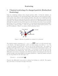
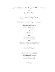
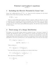
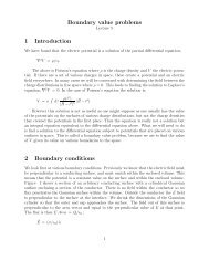
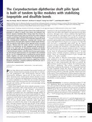
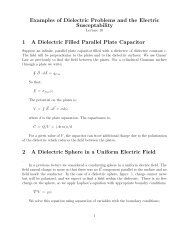
<strong><strong>Example</strong>s</strong> <strong>of</strong> <strong>magnetic</strong> <strong>field</strong> <strong>calculations</strong> <strong>and</strong><strong>applications</strong>Lecture 121 <strong>Example</strong> <strong>of</strong> a <strong>magnetic</strong> moment calculationWe consider the vector potential <strong>and</strong> <strong>magnetic</strong> <strong>field</strong> due to the <strong>magnetic</strong> moment created bya rotating surface charge, σ, on a cylinder. the geometry is shown in figure 1. The <strong>magnetic</strong>moment, I(area), <strong>of</strong> a small loop at the position, z as shown in the figure is ;d⃗m =σ(Rdθ dz)dt(πR 2 )ẑ = πσR 3 ω dz ẑThe vector potential is then;d ⃗ A = µ 04πd⃗m × ⃗rr 3 = µ 04π [πσR3 ω ẑ × ⃗rr 3This is integrated using ⃗r = ⃗α − ⃗z to get ⃗ A.⃗A =L/2∫−L/2d ⃗ AChoose ⃗α to lie in the (x, y) plane along the ˆx direction. Then ẑ × ⃗r = αŷ] dz⃗A = µ 04πd⃗m × ⃗rr 3 = [ µ 04π [πσR3 ωα]L/2∫−L/2dz 1[α 2 + z 2 ] 3/2]ŷ2 The <strong>field</strong> <strong>and</strong> action <strong>of</strong> a Quadrupole lensThe quadrupole <strong>field</strong> is illustrated by the <strong>magnetic</strong> <strong>field</strong> shown in figure 2 <strong>and</strong> given by theequations;B z = gxB x = gzB y = 0The <strong>field</strong> is generated by wire windings that create the <strong>magnetic</strong> poles shown in thefigure <strong>and</strong> parallel to the equipotential curves perpendicular to the <strong>field</strong> lines. We supposethe length <strong>of</strong> the <strong>field</strong> into the page is L, <strong>and</strong> the <strong>field</strong> lines are shown in the figure. The1
PrzωL/2αdmRσyx−L/2Figure 1: The vector potential <strong>of</strong> a rotating, cylindrical charge distributionzNSxSNFigure 2: A quadrupole magnet used to focus charged particles2
<strong>field</strong> strength increases linearly with distance from the axis.B 2 = B 2 x + B 2 z = g 2 r 2For positive particles moving with velocity ⃗ V into the page, the Lorentz force convergesa particle beam horizontally, <strong>and</strong> diverges it vertically. Check the force direction <strong>and</strong> notethe further away from the axis, the stronger the force. A <strong>magnetic</strong> lens is created if twoquadupole <strong>field</strong>s are placed in line <strong>and</strong> rotated by 90 deg with respect to each other. Thena proper choice <strong>of</strong> spacing, <strong>and</strong> <strong>field</strong> strength can provide focusing <strong>of</strong> a parallel beam <strong>of</strong>particles to a point some distance behind the two magnets.3 Power <strong>and</strong> the <strong>magnetic</strong> <strong>field</strong>The Lorentz force on a charge is ⃗ F = q[ ⃗ E + ⃗ V × ⃗ B]. This force causes the charge to movein a direction perpendicular to the <strong>field</strong> <strong>and</strong> velocity, ˆl. Then we determine the power dueto this movement.P = ⃗ V · ⃗F = q ⃗ V · ⃗EAs indicated, the force term involving the <strong>magnetic</strong> <strong>field</strong> vanishes, so the <strong>magnetic</strong> <strong>field</strong>does no work on a charge <strong>and</strong> cannot change its energy.4 Motion <strong>of</strong> a charged particle in a <strong>magnetic</strong> <strong>field</strong>We suppose a constant <strong>magnetic</strong> <strong>field</strong> in the ẑ direction, <strong>and</strong> a charged particle <strong>of</strong> mass, m,charge, q, <strong>and</strong> velocity, ⃗ V moves in this <strong>field</strong>. The motion is given by the Lorentz force,which in non-relativistic form, is given by;m d⃗ Vdt= q[ ⃗ V × ⃗ B]We neglect the interaction <strong>of</strong> the charge with other charges which may be present in abeam <strong>of</strong> such particles. In Cartesian coordinates the coupled equation set below is produced.dV xdtdV ydtdV zdt= V yqBm= −V xqBm= 03
The last equation requires that V z = constant. The first two equations may be decoupledgiving a second order ode.d 2 V idt 2= − qB m V iIn the above, V i represents V x or V y . The solution is harmonic, <strong>and</strong> to satisfy both firstorder equations;V x = V 0x cos(ωt + φ)V y = −V 0x sin(ωt + φ)Where ω = qB m <strong>and</strong> φ is a phase angle to be determined from the initial conditions.Assume that at t = 0 V x = V 0x <strong>and</strong> V y = 0. Then φ = 0 <strong>and</strong> A = V 0x . Now integrate theseequations again to get the coordinate trajectories. Let the initial velocity in the ẑ directionbe, V z = V 0z , <strong>and</strong> initial position be, (0, (V 0x /ω), Z 0 ).z = V 0z t + Z 0x = (V 0x /ω) sin(ωt)y = (V 0x /ω) cos(ωt)Substitution verifies these solutions <strong>and</strong> initial conditions. We observe the motion is ahelix in 3-D with a projection <strong>of</strong> circular motion onto the (x, y) plane. The radius <strong>of</strong> thiscircle, R, is ;x 2 + y 2 = R 2 = [V 0x /ω] 2In the above, R, represents the radius <strong>of</strong> curvature <strong>of</strong> the particle in the <strong>magnetic</strong> <strong>field</strong>.Insert the particle momentum projected onto the (x, y) plane, p.p = mV 0x = mωR = qBRR = pqB5 Drift Velocity <strong>and</strong> the Lorentz forceSuppose we apply a constant <strong>magnetic</strong> <strong>field</strong> in the ẑ direction <strong>and</strong> a constant electric <strong>field</strong>in the ˆx direction to a charged particle. The particle is initially at rest. The equations <strong>of</strong>motion in the (x, y) plane are;4
dV xdtdV ydt= qB m V y + (q/m) E 0= − qB m V xAfter application <strong>of</strong> the initial conditions, the solution has the form, with ω defined inthe previous section;V x = (q/mω) sin(ωt)V y = (q/mω)[cos(ωt) − 1]The position is obtained by a second integration;x = −(q/mω)[cos(ωt)/ω − 1] + X 0y = (q/mω)[sin(ωt)/ω − t] + Y 0In the above (X 0 , Y 0 ) is the initial position. This motion is strange as the circle centermoves with constant velocity in the ŷ direction. Now we study this a little further by placinga resistance, proportional to the velocity, to the motion <strong>of</strong> the charge. This is artificialbecause force is proportional to acceleration not velocity, but you have used frictional forcesproportional to velocity in mechanics, <strong>and</strong> here I want an energy disipating term. Thus Iadd a term which contains the first odd derivative <strong>of</strong> the position, velocity. Introduction <strong>of</strong>the force term σ ⃗ V into the above equations gives;dV xdtdV ydt+ σ/m V x = qB m V y + (q/m) E 0+ σ/m V y = − qB m V xWe look for the equilibrum solution, ie the solution when the velocity becomes independent<strong>of</strong> time so dV idt = 0.V x =V y =qσσ 2 + (qB) 2 E 0q 2 Bσ 2 + (qB) 2 E 0The drift angle between the applied <strong>field</strong> <strong>and</strong> the motion is called the Lorentz angle <strong>and</strong>is given by;tan(θ) = V y /V x = −qB/σ5
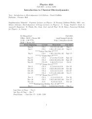
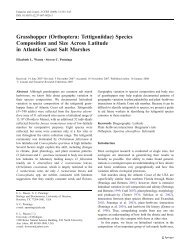
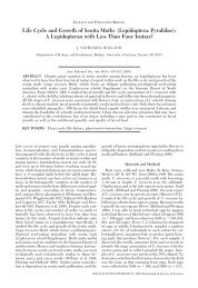
IVadlbBFigure 3: The geometry describing the Hall effectThe particle drifts at a constant velocity at the angle θ with respect to the applied <strong>field</strong>.The above examples give a few simple illustrations <strong>of</strong> the motion <strong>of</strong> charged particles in<strong>magnetic</strong> <strong>field</strong>s. In general, this topic is treated in magnetohydrodynamics (Plasmas) <strong>and</strong>the motion is highly non-linear <strong>and</strong> non-intuitive. The underst<strong>and</strong>ing <strong>of</strong> plasma is crucial tothe development <strong>of</strong> controlled fusion reactors.6 The Hall effectWe suppose a current through a conducting medium in which there is a <strong>magnetic</strong> <strong>field</strong> perpendicularto the current flow <strong>and</strong> the surfaces <strong>of</strong> the conductor figure 3. The currentrepresents a flow <strong>of</strong> charge so that there is a deflection <strong>of</strong> the current due to the Lorentzforce. As previously determined Idl = qV so the force on a small element <strong>of</strong> current due tothe <strong>magnetic</strong> <strong>field</strong> when the <strong>magnetic</strong> <strong>field</strong> <strong>and</strong> the current are perpendicular is;dF m = IBdlCharge flows <strong>and</strong> builds up an electric <strong>field</strong> on the parallel surfaces <strong>of</strong> the conductor.When equilibrum is reached, the electric force cancells the <strong>magnetic</strong> force.⃗F = 0 = q[ ⃗ E + ⃗ V × ⃗ B]In this case;q(dE) = −d(V/w) IBdlThe charge per unit volume in the conductor as obtained from the figure is ρ = q/ab(dl).Substitute for q <strong>and</strong> let dE = V/b, with V the potential between the sides <strong>of</strong> the conductor.6
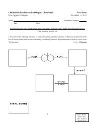
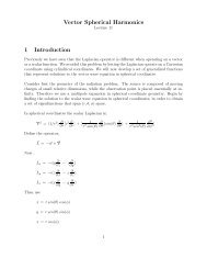
z^ ^φ φz’ θ Pr’b θ rbaRFigure 4: The geometry to find the <strong>magnetic</strong> <strong>field</strong> inside a cylindrical cavity in a cylindricalconductorThen;V = −IB/(ρa)The hall effect occurs for all current flow in a <strong>magnetic</strong> <strong>field</strong> <strong>and</strong> is used in a number <strong>of</strong>instruments to measure either currents or <strong>magnetic</strong> <strong>field</strong>s.7 <strong>Example</strong> <strong>of</strong> Ampere’s law <strong>and</strong> superpositionThere is a current flow in a cylindrical conductor <strong>of</strong> radius, R. The conductor has a hole<strong>of</strong> radius, a, displaced a distance, b from the axis <strong>of</strong> the conductor. The geometry is shownin figure 4. We are to find the <strong>magnetic</strong> <strong>field</strong> in the hole. This is done by superpositionas shown in the figure. For the solid conductor the current density is J ⃗ C = Iπ[R 2 − a 2 ]ẑ.We subtract the <strong>field</strong> due to the current density <strong>of</strong> the hole J ⃗ H =Iπ[R 2 2 Now apply− a ]ẑ.Ampere’s law to get the <strong>field</strong> <strong>of</strong> each cylindrical conductor at a <strong>field</strong> point, P, shown in figure4.∮ ⃗B · d ⃗ l =µ 04π IFor the conducting cylinder, the enclosed current is; I c = J c (πr 2 ). The circulation onthe left side <strong>of</strong> the above integral is evaluated to be B(2πr). Thus⃗B C =µ 0 I πr 2π(R 2 − a 2 ) 2πr ˆφ C =µ 0 Ir2π(R 2 − a 2 ) ˆφ C7
In the same way the <strong>field</strong> for the current creating the hole is;⃗B H =µ 0 Ir ′2π(R 2 − a 2 ) ˆφ HThe geometry is shown in the figure. We subtract these vector <strong>field</strong>s. Write the unitvectors ˆφ C <strong>and</strong> ˆφ H in Cartesian coordinates <strong>and</strong> use the geometry to obtain;ˆφ H = −sin(θ ′ )ẑ − cos(θ ′ )ˆxˆφ C = cos(θ)ẑ − sin(θ)ˆxr ′ = z ′ /cos(θ ′ ) = α/sin(θ ′ )r = z/cos(θ) = α/sin(θ)Since z − z ′ = b the final result is;B =µ 0 Ib2π(R 2 − a 2 )As an alternative use ⃗rˆφ c = ⃗r × dˆl <strong>and</strong> the equivalent expression for the primed coordinates<strong>and</strong> subtract to get ⃗ b. Thus the <strong>magnetic</strong> <strong>field</strong> is constant in the interior <strong>and</strong> pointedin the ẑ direction.8 Magnetic pressure <strong>and</strong> energyConsider two parallel current sheets separated by a distance, d, with uniform, constant currentsflowing in opposite directions, figure 5. We find the <strong>magnetic</strong> <strong>field</strong> due to one <strong>of</strong>these sheets on the other. The <strong>magnetic</strong> <strong>field</strong> is obtained using Ampere’s law as previously.Because <strong>of</strong> symmetry the <strong>magnetic</strong> <strong>field</strong> must be directed parallel to the sheet, <strong>and</strong> can onlydepend on the perpendicular distance from the sheet to the <strong>field</strong> point. Evaluation <strong>of</strong> theintegral form <strong>of</strong> Ampere’s law gives;∮ ⃗B · d ⃗ l = 2BL = µ0 IThe factor <strong>of</strong> 2 coming from the <strong>field</strong> above <strong>and</strong> below the sheet, <strong>and</strong> L being the distanceparallel to the sheet over the path along ⃗ B. I is the current that flows through thisAmperian loop. Thus for one sheet;8
LI/LBBBBBdI/LFigure 5: The <strong>magnetic</strong> <strong>field</strong> created by 2 parallel current sheets with currents flowing inopposi te directionsB = µ(I/L)/2 = (µ/2) IIn the above we have written I as the current per unit width on the sheet. The direction<strong>of</strong> the <strong>magnetic</strong> <strong>field</strong> is given by the right-h<strong>and</strong>-rule. Note that the <strong>field</strong> is independent <strong>of</strong>the distance from the sheet. Thus the <strong>field</strong>s when superimposed from the two sheets, addbetween the sheets <strong>and</strong> cancel outside the sheets. Finally we also see that the force generatedby the <strong>magnetic</strong> <strong>field</strong> on one sheet interacting with the current on the other is repulsive. Wevisualize this situation by thinking <strong>of</strong> the <strong>magnetic</strong> <strong>field</strong> as creating a pressure between theplates tending exp<strong>and</strong> the distance between them.Use the Lorentz force to calculate this force. In the equation for the Lorentz force,substitute IL for qV . The <strong>field</strong> <strong>and</strong> current direction are perpendicular, so F 2 = I 2 LB 1 =I 2 x 2 (µ/2)I 1 . Now the total <strong>magnetic</strong> <strong>field</strong> between the plates comes from the superposition<strong>of</strong> both <strong>field</strong>s which add to B T = 2(µ/2)I 1,2 . Then I 1,2 = BL/µ which we substitute for I 1in the force equation yielding;FLx = 12µ 0B 2The above is the force per unit surface area (pressure) <strong>of</strong> one current sheet on the other.This pressure attempts to push the plates apart. Now suppose we do work against this pressureby compressing the plates a distance, d. The movment <strong>of</strong> the plates removes a volume<strong>of</strong> the <strong>magnetic</strong> <strong>field</strong>, Lxd, under the Amperian loop. <strong>and</strong> puts an energy into the systemgiven by W = Fd. We remove the geometry in the equation by dividing by the volume toobtain the energy per unit volume which we assign to the <strong>magnetic</strong> <strong>field</strong>. If we allow theplates to re-exp<strong>and</strong>, the plates do work removing this energy creating additional <strong>field</strong> in thisvolume. Compare this energy density, (1/2µ 0 )B 2 , to the energy density <strong>of</strong> the electric <strong>field</strong>,(ǫ 0 /2)E 2 .9
∮ ⃗B · d ⃗ l = µ0 I TIBFigure 6: The geometry to find <strong>field</strong> enclosed in a torus using Ampere’s law9 Additional <strong><strong>Example</strong>s</strong>9.1 Field <strong>of</strong> a torusThe geometry <strong>of</strong> a torus is illustrated in figure 6. We assume that a current sheet movingin a circular direction around the donught is continuous, (ie very tightly wound wires). N<strong>of</strong>ield leaks out <strong>of</strong> the donught, <strong>and</strong> the geometry is symmetric in azimuthal angle. Thus wecan use Ampere’s law to get the <strong>magnetic</strong> <strong>field</strong>. Use a circular Amperian loop as shown;B = µ 02πrIn this expression I T is the total current flowing. We could write a current per unitwidth <strong>of</strong> I = I T2πrto remove the geometric dependence.9.2 Field <strong>of</strong> a bipolar filamentWe assume two long filaments carring a current I in opposite directions. We are to find thevector potential, ⃗ A, for this geometry, figure 7. By symmetry, ⃗ A, must be independent <strong>of</strong>z. We have;10
zIdzrR1xzR2IyFigure 7: The geometry to find the vector potential created by two long, parallel filaments<strong>of</strong> current flowing in opposite directions⃗A = µ 04π∫dτ⃗ JrThe current density is in the direction <strong>of</strong> ẑ <strong>and</strong> use J ⃗ · d area ⃗ .⃗A = µ ∞∫04π ẑ [ dz∞∫−∞ (R2 2 + z2 ) 1/2 − √⃗A = 2 µ 04π I ln[z + z 2 + R22 √ ] ∞z + z 2 + R12 0 ẑ⃗A = 2 µ 04π I ln[R 1R 2]−∞dz(R 1 2 + z2 ) 1/2]11