Complexity-Optimized Low-Density Parity-Check Codes

Complexity-OptimizedLow-Density Parity-Check CodesMasoud ArdakaniDepartment of Electrical & Computer EngineeringUniversity of Alberta, ardakani@ece.ualberta.caBenjamin Smith, Wei Yu, Frank R. KschischangDepartment of Electrical & Computer EngineeringUniversity of Toronto, {ben, weiyu, frank}@comm.utoronto.caAbstractUsing a numerical approach, tradeoffs between code rate and decoding complexityare studied for long-block-length irregular low-density parity-check codesdecoded using the sum-product algorithm under the usual parallel-update messagepassingschedule. The channel is an additive white Gaussian noise channel and themodulation format is binary antipodal signalling, although the methodology canbe extended to any other channels for which a density evolution analysis may becarried out. A measure is introduced that incorporates two factors that contributeto the decoding complexity. One factor, which scales linearly with the number ofedges in the code’s factor graph, measures the number of operations required tocarry out a single decoding iteration. The other factor is an estimate of the numberof iterations required to reduce the the bit-error probability from that given by thechannel to a desired target. The decoding complexity measure is obtained from adensity-evolution analysis of the code, which is used to relate decoding complexitywith the code’s degree distribution and code rate. One natural optimizationproblem that arises in this context is to maximize code rate for a given channelsubject to a constraint on decoding complexity. At one extreme (no constraint ondecoding complexity) one obtains the “threshold-optimized” LDPC codes that havebeen the focus of much attention in recent years. Such codes themselves representone possible means of trading decoding complexity for rate, as such codes can beapplied in channels better than the one for which they are designed, achieving thebenefit of a reduced decoding complexity. However, it is found that the codes optimizedusing the methods described in this paper provide a better tradeoff, oftenachieving the same code rate with approximately 1/3 the decoding complexity ofthe threshold-optimized codes.1 IntroductionThe problem of designing capacity-approaching irregular low-density parity-check (LDPC)codes under different decoding algorithms and channel models has been studied extensively(e.g., as a starting point, see [1, 2, 3]). The usual design objective is to find acode degree distribution that maximizes the decoding threshold (e.g., the largest noisevariance for which successful decoding is possible) for a given rate or, equivalently, to

find a degree distribution that maximizes the code rate for a given decoding threshold.In practice, however, such codes would require an impractically large number of decodingiterations. In fact, for decoding algorithms with the property that message distributionscan be described by a single parameter, it is proved that, in the limit, the required numberof iterations for convergence approaches infinity as the rate of the code increases [4].As a result, a threshold-optimized code in practice must be used over a channel different(better) than the one for which the code is designed.The problem with the threshold-optimization approach is that decoding complexityis not considered in the process of code design. Put another way, if one wishes to designa practically-decodable code, it may be best to further trade the decoding threshold fora more desirable decoding trajectory. If decoding complexity could be incorporated inthe design process, one could find the highest-rate code for a certain affordable level ofcomplexity on a given channel condition or, the code with the minimum decoding complexityfor a required rate and a given channel condition. Clearly, these design objectivesbetter reflect the requirements of practical communication-system design. Towards thisend, we show in this paper how the decoding complexity of an irregular LDPC code canbe related to its degree distribution. We then formulate a methodology that is capableof finding low-complexity degree distributions for a given code rate and channel.Understanding the performance/complexity tradeoff has always been a central issuein coding theory. In recent years, particularly since the discovery of capacity-approachingcodes, “performance” has come to mean the achievable code rate. For the binary erasurechannel (BEC), the rate/complexity issue is addressed by Shokrollahi [5] for LDPC codes,and by Khandekar and McEliece [6] and also Sason and Urbanke [7] for irregular repeataccumulatecodes. Decoding the output of an erasure channel is quite different thandecoding the output of a noisy channel, as the decoding procedure operates via an edgedeletionprocess, whose complexity scales linearly with the number of edges in the code’sfactor graph. However, for other channel models, decoding is an iterative process, and soa decoding complexity measure must also scale with the required number of iterations.This observation has previously been made in the work of Richardson and Urbanke [2],where a numerical design procedure for irregular LDPC codes involving a measure of thenumber of iterations is proposed. Recently, in [8], we studied this problem for LDPCcoding under Gallager’s decoding Algorithm B [9] over the binary symmetric channel.The results of [8] rely on the one-dimensional nature of decoding Algorithm B. Thispaper addresses complexity-based designs for the general binary-input symmetric-outputchannels, and symmetric decoding. That is to say, as long as a density evolution analysisof the decoder is possible, our method of complexity optimization is applicable.In this work, although the decoding complexity of an LDPC code is related to itsdegree distribution via a one-dimensional representation of the decoder, the results arenot based on a one-dimensional analysis. We use density evolution for the analysis, yetrepresent the convergence behavior in a one-dimensional format that we call an extrinsicinformation transfer (EXIT) chart (despite the fact that it tracks the message error raterather than the mutual information, and the fact that it is based on a density evolutionanalysis instead of a Gaussian approximation). A one-dimensional representation plays acentral role in the formulation of the code-design problem [10] as well as in the formulationof complexity in terms of the code degree distribution [8].The rest of this paper is organized as follows. In Sections 2 and 3, we briefly reviewelementary EXIT charts and their role in irregular LDPC code design as well as a methodfor obtaining elementary EXIT charts through density evolution. In Section 4 we define

the decoding complexity and we present a formula which relates the degree distribution ofthe code to its decoding complexity for achieving a certain target error rate. In Section 5,the optimization problem is formulated and the optimization methodology is described.The numerically optimized degree distributions and the complexity-performance tradeoffcurves for a Gaussian channel are presented in Section 6 and the paper is concluded inSection 7.2 PreliminariesFollowing the notation of [1], we define an ensemble of irregular LDPC codes by itsvariable-degree distribution {λ 2 , λ 3 , . . .} and its check-degree distribution {ρ 2 , ρ 3 , . . .},where λ i denotes the fraction of edges incident on variable nodes of degree i and ρ jdenotes the fraction of edges incident on check nodes of degree j. If all the parityconstraints are linearly independent, it is easy to see that the rate of an irregular LDPCcode is related to its degree distribution by∑R(λ, ρ) = 1 −∑iρ ii iλ ii. (1)If, due to the random construction of the code, some of the parity check constraints arelinearly dependent, the actual rate of the code will be slightly higher.There are many decoding algorithms available for LDPC codes. If the decoding algorithmand the channel satisfy some symmetry properties [11], performance of a givencode can be studied by density evolution. The inputs to the density evolution algorithm[11] are the probability density function (pdf) of channel log-likelihood ratio (LLR) messages1 and the pdf of the extrinsic LLR messages from the previous iteration. The outputis the pdf of the extrinsic LLR messages at the current iterations. This density will beused as input for finding the message density in the next iteration. The negative tail ofthe LLR density is the message error rate. If decoding is successful, this tail vanishes asthe number of iterations tends to infinity.In the above discussion, one iteration is defined as one round of message updates atboth the check nodes and the variable nodes. In other words, the input to one iterationis the messages sent from variable nodes to check nodes and the output is the same set ofmessages after being updated at check nodes and variable nodes. We assume that theseupdates occur in parallel, even though it is possible that a serial updating schedule mayresult in fewer iterations.3 EXIT chart representation of density evolutionAn EXIT chart based on message error rate is motivated by Gallager’s decoding AlgorithmB [9]. Using Algorithm B to decode a regular LDPC code, it is easy to establisha recursive equation that provides an exact description of the message error rate after agiven number of iterations. In this case, a p in vs. p out EXIT chart is precisely a graphicalrepresentation of this equation.With this in mind, from density evolution we may obtain a p in vs. p out EXIT chartfor an arbitrary channel and decoder pair as follows. After performing N iterations of1 Under the assumption that the all-zero codeword is transmitted.

density evolution, one can visualize the convergence behavior of the decoder by plottingthe extrinsic message error rate of iteration m, m ∈ {1, 2, · · · , N} (let us call this p (m) )vs. the extrinsic message error rate of iteration m − 1, i.e., p (m−1) . This resembles theEXIT chart analysis of [12], hence we call it an EXIT chart. This can also be representedas a mapping (a function)p (m) = f(p (m−1) , λ, ρ), m ∈ {1, 2, · · · , N}. (2)Notice that the above defined method results in an EXIT chart which is defined on Ndiscrete points. Also notice that f as well as its domain and range are influenced by thecode parameters λ and ρ. Nevertheless, using Bayes’ rule we havep (m) = ∑ iλ i · p (m)i , (3)where p (m)i is the message error rate at the output of degree i variable nodes at iterationm. Equation (3) can be rewritten asf(p, λ, ρ) = ∑ iλ i · f i (p, λ, ρ), (4)where f i (p, λ, ρ) can be thought as an EXIT chart associated with degree i nodes. Thisis similar to elementary EXIT charts of [4], where the EXIT chart of an irregular codedecomposes as a linear combination of EXIT charts of left-regular codes. This reducesthe problem of code design to the problem of shaping an EXIT chart out of some precomputedelementary EXIT charts. It is evident here that elementary EXIT charts arecentral to the formulation of the optimization problem of interest.However, as the elementary EXIT charts of (4) are functions of λ, the EXIT chart ofthe code is affected by λ k in two ways. One is through the linear combination of (4) asa multiplying factor and the other one is the effect of λ on f i (p, λ, ρ)’s, i.e.,∂f(p, λ, ρ)∂λ k= f k (p, λ, ρ) + ∑ iλ i∂f i (p, λ, ρ)∂λ k. (5)In practice, the first term on the right hand of (5) is much larger than the second term.Therefore, as long as λ undergoes a small change, we may disregard the dependency ofelementary EXIT charts on λ. Fixing ρ, (4) can be simplified tof(p) = ∑ iλ i · f i (p), (6)which is equivalent to the formulation of [4]. However, due to the dependency of elementaryEXIT charts on λ, they have to be updated when λ undergoes a large change.Another technical issue (which arises here but not in the case of Algorithm B) is thatthe elementary EXIT charts cannot be computed individually from left-regular codes.There are two reasons for this. First of all, the probability distribution associated withAlgorithm B can be described by a single parameter. Therefore, a particular value of p inmaps to a unique input distribution. However, in the case of the Gaussian channel, theinput distribution at a particular value of p in is dependent on λ, and can only be obtainedby performing full density evolution on the entire code at once. Secondly, analysis ofAlgorithm B provides an explicit formula for the left-regular elementary EXIT charts.

Therefore, a component code that may not converge on its own during density evolution,say a code which has exclusively degree-two variable nodes, nevertheless has an explicitrepresentation that allows one to construct a p in vs. p out curve over its entire domain.For the case of the Gaussian channel, if one conducts density evolution on an elementarydegree-two variable code, the process would fail to converge for most cases of interest,preventing us from obtaining an elementary EXIT chart defined over the full domain ofp in .To overcome these problems, we obtain elementary EXIT charts by running densityevolution for the irregular code. At each iteration, we find the LLR message pdf at theoutput of variable nodes of different degrees, and we extract the LLR message error rate(negative tail of pdf) for each variable node degree. This forms f i (p, λ, ρ). Here, it isassumed that the irregular code will converge to the specified target error rate, whichguarantees that the elementary EXIT charts are defined over a discrete set of p such thatmin(p) ≤ p t , where p t is the target error rate specified in the code design problem. Thisallows for shaping an EXIT chart of desired properties over the range of interest. Byinterpolating, one can acquire a continuous version of the elementary EXIT charts overthe interval [p t , p 0 ], where p 0 is the initial message error rate (from the channel messages)and p t is the target error rate.4 Decoding Complexity AnalysisIn this section, we first study the decoding complexity per iteration, and then we analyzethe required number of iterations for a target error rate.4.1 Decoding complexity per iterationFor a message-passing decoder, it is not hard to see that the decoding complexity periteration scales roughly linearly with the number of edges. This is because each edgecarries a message, and each message has to be updated at each iteration, and suchan update requires essentially constant computational effort. A detailed study of thiscomplexity for the sum-product decoding (which can be extended to general messagepassingrules) is as follows.At a variable node of degree d v , a maximum of 2d v operations is enough to computeall the output messages. Notice that at each variable node, one can add all d v + 1 inputLLR messages in d v operations. To compute each outgoing message, one subtraction isrequired. Since d v outgoing messages should be computed, the total number of operations(addition and subtraction) per iteration at the variable nodes is 2 ∑ v d v, or equivalently2E, where E is the number of edges in the graph.Similarly, at a check node of degree d c , a total of 2d c − 1 operations is needed. Thenumber of operations can be counted as follows: first (d c − 1) products (of tanh) needto be performed, then one division per outgoing message (taking tanh and atanh is notconsidered as an operation). Since there are d c outgoing messages, the total number ofoperations is 2d c −1, which results in a total of 2E −C operations, where C is the numberof check nodes.The overall complexity per iteration is then 4E − C, which is roughly proportionalto E, since usually 4E ≫ C. Therefore, in this work we assume that the complexityper iteration is simply proportional to E. This complexity has to be normalized perinformation bit to be meaningful. The complexity per information bit per iteration is

then proportional toERn , (7)where R is the code rate and n is the block length.4.2 Analysis of Number of IterationsAs mentioned earlier, for the binary erasure channel, since decoding is an edge deletionprocess, the total complexity is measured as the number of edges. However, in all othermessage-passing decoding algorithms, the number of iterations directly affects the totaldecoding complexity. The complexity discussion in the previous section was only for oneiteration. Considering N decoding iterations, from (7) and (1), the overall complexityper information bit, X, can be measured asX =N∑i λ i/i − ∑ i ρ i/i . (8)Therefore, to find the total complexity, the required number of iterations, N, should beestimated.The number of iteration strongly depends on the shape of the EXIT chart f(p) andthe target message error rate. It is shown in [8] that the number of required iterationscan be closely approximated asN =∫ p0p tdp(p logpf(p)). (9)This formula is a very accurate estimate of the number of iterations for a wide range off(p)’s. Some examples are provided in [8].We finish this section by rewriting (8), explicitly in terms of the code degree distribution.That isX(λ, ρ) =1∑i λ i/i − ∑ i ρ i/i∫ p0p tdp(p log∑pi λ if i (p)). (10)It is also shown in [8] that for a fixed ρ this complexity measure is a convex function ofλ over the set { ( ∑ )}1λ : ∀pe ≤ λi f i (p)≤ 1 .2 p5 Optimization MethodologyFollowing the approach of [8], we minimize the complexity of a code subject to a rateconstraint. By varying the target rate and solving the sequence of optimization problems,we obtain the complexity-rate tradeoff curve.For simplicity, let us assume that ρ is fixed. There exists convincing evidence thatconventional rate/threshold optimization techniques are not very sensitive to ρ. Forinstance, it is shown that codes with regular check degree can achieve the capacity ofthe binary erasure channel [5] and can perform very close to the Shannon limit on theGaussian channel [10]. Recall that the fixed ρ assumption, together with the assumptionof keeping λ in a small region of space, results in (6), which defines a linear relation

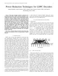
40003500Complexity−Rate Optimized CodesThreshold Optimized Codes3000Complexity per Information Bit250020001500100050000.47 0.48 0.49 0.5 0.51 0.52 0.53 0.54 0.55Rate (bits/transmission)Figure 1: Complexity-rate tradeoff on an AWGN channel with noise σ = 0.9 for an irregularLDPC code with check degree 9 and sum-product decoding. The lower curve is the complexity-rateoptimized code design. The upper curve is produced by designing the highest threshold code foreach rate.6 Numerical Results and DiscussionIn this section, we present the results of our numerical optimization on a binary-inputadditive white Gaussian noise channel with noise σ = 0.9. The target error rate is set to10 −7 . To allow for a fair comparison between our design method and conventional designmethods, threshold optimized codes of different rates, as produced by LdpcOpt [13], aretested on the channel of study and their rate is plotted versus their complexity in Fig.1. The results of the rate-complexity tradeoff after performing our optimization are alsoplotted on the same figure. As can be seen, the new code-design technique results insignificantly more efficient codes. In many cases, the decoding complexity is reduced bya factor of three or more. All the codes are limited to a maximum variable node degreeof 30. Additionally, regular check degrees of degree 8, 9 and 10 were used. The plottedresults consist of the best of the three codes at each value of the rate. Table 1 comparesthe degree distribution of a rate half code found through the new optimization techniquefor the above channel, with a rate half code found through conventional design methods.Both codes have a regular check degree of 9.Fig. 2(a) compares the EXIT charts of the codes presented in Table 1. Fig. 2(b) showsthe same EXIT charts but in log scale. Observe that the rate-complexity optimized codehas a tighter EXIT chart in the earlier iterations and a wider EXIT chart at the lateriterations. It is proved in [4] that, for a wide class of decoding algorithms, when the EXITchart of two codes, f (1) (p) and f (2) (p) satisfy f (1) (p) ≥ f (2) (p), ∀p ∈ (0, p 0 ] then f (1) (p)corresponds to a higher rate. Also in [14] it is proved that for the binary erasure channel,the area underneath the EXIT chart scales with the code rate. In this example, since bothcodes have the same rate, one EXIT chart cannot dominate the other one everywhere,but the optimization program carefully trades the area underneath the EXIT chart forthe complexity. By opening up the EXIT chart close to the origin, we do not expect a

Deg. TO RCO Deg. TO RCO Deg. TO RCO2 0.2124 0.0623 11 0.0000 0.0173 19 0.0000 0.02553 0.1985 0.4948 12 0.0000 0.0260 20 0.0003 0.02175 0.0084 0.0000 13 0.0000 0.0313 21 0.0000 0.01766 0.0747 0.0000 14 0.0000 0.0340 22 0.0000 0.01327 0.0142 0.0000 15 0.0000 0.0346 23 0.0000 0.00868 0.1665 0.0118 16 0.0000 0.0337 24 0.0000 0.00389 0.0091 0.0000 17 0.0000 0.0317 25 0.0000 0.000810 0.0200 0.0048 18 0.0000 0.0288 30 0.2959 0.0975Table 1: Degree distributions of two rate-1/2 codes, one optimized for threshold (TO) and theother optimized for rate and complexity (RCO). Total decoding complexity per information bit isestimated at 1143 (with 127 iterations) for the former and 342 (with 38 iterations) for the latter.significant rate loss, yet we obtain a significant complexity gain. The small rate loss isthen compensated for by slightly tightening up the EXIT chart in early iterations (whichhave no considerable impact on the complexity).0.14Threshold Optimized CodeComplexity−Rate Optimized CodeThreshold Optimized CodeComplexity−Rate Optimized Code10 0 Pin0.120.110 −20.08PoutPout10 −40.060.0410 −60.0200 0.02 0.04 0.06 0.08 0.1 0.12 0.14Pin(a)10 −810 −6 10 −4 10 −2 10 0(b)Figure 2: EXIT charts for complexity-rate optimized codes: (a) linear scale, (b) log scale.7 Concluding RemarksThis paper proposes a new LDPC code-design objective based on a joint optimization ofrate and complexity. The paper argues that the conventional LDPC code-design whichmaximizes the code rate alone is not the best approach for practical purposes. The centralobservation is that, through a one-dimensional representation of convergence behavior,the decoding complexity of an irregular LDPC code can be related to its degree distributionin a closed form, hence a joint optimization of rate and complexity is possible. Ourtechnique is applicable to all binary-input symmetric-output channels, where a densityevolution analysis is possible. Numerical results on a Gaussian channel show substantialcomplexity reduction using the new optimization technique.

References[1] M. G. Luby, M. Mitzenmacher, M. A. Shokrollahi, and D. A. Spielman, “Improvedlow-density parity-check codes using irregular graphs,” IEEE Transactions on InformationTheory, vol. 47, no. 2, pp. 585–598, Feb. 2001.[2] T. J. Richardson, M. A. Shokrollahi, and R. L. Urbanke, “Design of capacityapproachingirregular low-density parity-check codes,” IEEE Transactions on InformationTheory, vol. 47, no. 2, pp. 619–637, Feb. 2001.[3] S.-Y. Chung, G. D. Forney Jr., T. J. Richardson, and R. L. Urbanke, “On thedesign of low-density parity-check codes within 0.0045 dB of the Shannon limit,”IEEE Communications Letters, vol. 5, no. 2, pp. 58–60, Feb. 2001.[4] M. Ardakani, T. H. Chan, and F. R. Kschischang, “EXIT-Chart properties of thehighest-rate LDPC code with desired convergence behavior,” IEEE CommunicationsLetters, vol. 9, no. 1, pp. 52–54, Jan. 2005.[5] A. Shokrollahi, “New sequence of linear time erasure codes approaching the channelcapacity,” in Proc. the International Symposium on Applied Algebra, Algebraic Algorithmsand Error-Correcting Codes, no. 1719, Lecture Notes in Computer Science,1999, pp. 65–67.[6] A. Khandekar and R. J. McEliece, “On the complexity of reliable communicationon the erasure channel,” in Proc. IEEE International Symposium on InformationTheory, 2001, p. 1.[7] I. Sason and R. Urbanke, “Complexity versus performance of capacity-achieving irregularrepeat-accumulate codes on the binary erasure channel,” IEEE Transactionson Information Theory, vol. 50, no. 6, pp. 1247–1256, June 2004.[8] W. Yu, M. Ardakani, B. Smith, and F. R. Kschischang, “Complexity-optimizedLDPC codes for Gallager decoding algorithm B,” in Proc. IEEE International Symposiumon Information Theory, Adelaide, Australia, Sept. 2005.[9] R. G. Gallager, Low-Density Parity-Check Codes. Cambridge, MA: MIT Press,1963.[10] M. Ardakani and F. R. Kschischang, “A more accurate one-dimensional analysis anddesign of LDPC codes,” IEEE Transactions on Communications, vol. 52, no. 12, pp.2106–2114, Dec. 2004.[11] T. J. Richardson and R. L. Urbanke, “The capacity of low-density parity-checkcodes under message-passing decoding,” IEEE Transactions on Information Theory,vol. 47, no. 2, pp. 599–618, Feb. 2001.[12] S. ten Brink, “Convergence behavior of iteratively decoded parallel concatenatedcodes,” IEEE Transactions on Communications, vol. 49, pp. 1727–1737, Oct. 2001.[13] R. L. Urbanke, “LdpcOpt: a fast and accurate degree distribution optimizer forLDPC code ensembles,” online: lthcwww.epfs.ch/research/ldpcopt.[14] A. Ashikhmin, G. Kramer, and S. ten Brink, “Extrinsic information transfer functions:a model and two properties,” in Proc. Conference on Information Sciencesand Systems, Princeton, USA, Mar. 2002, pp. 742–747.