v2010.10.26 - Convex Optimization

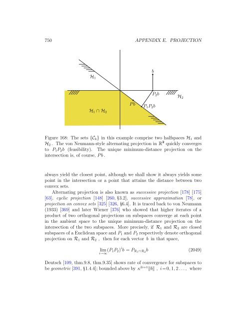
750 APPENDIX E. PROJECTIONbH 1H 2P 2 bH 1 ∩ H 2PbP 1 P 2 bFigure 168: The sets {C k } in this example comprise two halfspaces H 1 andH 2 . The von Neumann-style alternating projection in R 2 quickly convergesto P 1 P 2 b (feasibility). The unique minimum-distance projection on theintersection is, of course, Pb .always yield the closest point, although we shall show it always yields somepoint in the intersection or a point that attains the distance between twoconvex sets.Alternating projection is also known as successive projection [178] [175][63], cyclic projection [148] [260,3.2], successive approximation [78], orprojection on convex sets [325] [326,6.4]. It is traced back to von Neumann(1933) [369] and later Wiener [376] who showed that higher iterates of aproduct of two orthogonal projections on subspaces converge at each pointin the ambient space to the unique minimum-distance projection on theintersection of the two subspaces. More precisely, if R 1 and R 2 are closedsubspaces of a Euclidean space and P 1 and P 2 respectively denote orthogonalprojection on R 1 and R 2 , then for each vector b in that space,lim (P 1P 2 ) i b = P R1 ∩ R 2b (2049)i→∞Deutsch [109, thm.9.8, thm.9.35] shows rate of convergence for subspaces tobe geometric [391,1.4.4]; bounded above by κ 2i+1 ‖b‖ , i=0, 1, 2..., where