v2010.10.26 - Convex Optimization

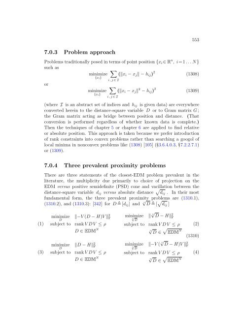
5537.0.3 Problem approachProblems traditionally posed in terms of point position {x i ∈ R n , i=1... N }such as∑minimize (‖x i − x j ‖ − h ij ) 2 (1308){x i }orminimize{x i }i , j ∈ I∑(‖x i − x j ‖ 2 − h ij ) 2 (1309)i , j ∈ I(where I is an abstract set of indices and h ij is given data) are everywhereconverted herein to the distance-square variable D or to Gram matrix G ;the Gram matrix acting as bridge between position and distance. (Thatconversion is performed regardless of whether known data is complete.)Then the techniques of chapter 5 or chapter 6 are applied to find relativeor absolute position. This approach is taken because we prefer introductionof rank constraints into convex problems rather than searching a googol oflocal minima in nonconvex problems like (1308) [105] (3.6.4.0.3,7.2.2.7.1)or (1309).7.0.4 Three prevalent proximity problemsThere are three statements of the closest-EDM problem prevalent in theliterature, the multiplicity due primarily to choice of projection on theEDM versus positive semidefinite (PSD) cone and vacillation between thedistance-square variable d ij versus absolute distance √ d ij . In their mostfundamental form, the three prevalent proximity problems are (1310.1),(1310.2), and (1310.3): [342] for D [d ij ] and ◦√ D [ √ d ij ](1)(3)minimize ‖−V (D − H)V ‖ 2 FDsubject to rankV DV ≤ ρD ∈ EDM Nminimize ‖D − H‖ 2 FDsubject to rankV DV ≤ ρD ∈ EDM Nminimize ‖ ◦√ D − H‖◦√ 2 FDsubject to rankV DV ≤ ρ◦√ √D ∈ EDMNminimize ‖−V ( ◦√ D − H)V ‖◦√ 2 FDsubject to rankV DV ≤ ρ◦√ √D ∈ EDMN(2)(1310)(4)