v2010.10.26 - Convex Optimization

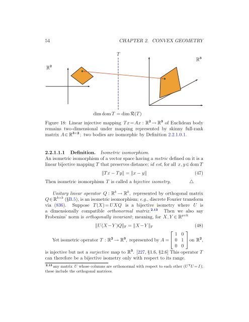
54 CHAPTER 2. CONVEX GEOMETRYTR 2 R 3dim domT = dim R(T)Figure 18: Linear injective mapping Tx=Ax : R 2 → R 3 of Euclidean bodyremains two-dimensional under mapping represented by skinny full-rankmatrix A∈ R 3×2 ; two bodies are isomorphic by Definition 2.2.1.0.1.2.2.1.1.1 Definition. Isometric isomorphism.An isometric isomorphism of a vector space having a metric defined on it is alinear bijective mapping T that preserves distance; id est, for all x,y ∈dom T‖Tx − Ty‖ = ‖x − y‖ (47)Then isometric isomorphism T is called a bijective isometry.Unitary linear operator Q : R k → R k , represented by orthogonal matrixQ∈ R k×k (B.5), is an isometric isomorphism; e.g., discrete Fourier transformvia (836). Suppose T(X)= UXQ is a bijective isometry where U isa dimensionally compatible orthonormal matrix. 2.13 Then we also sayFrobenius’ norm is orthogonally invariant; meaning, for X,Y ∈ R p×k‖U(X −Y )Q‖ F = ‖X −Y ‖ F (48)⎡ ⎤1 0Yet isometric operator T : R 2 → R 3 , represented by A = ⎣ 0 1 ⎦on R 2 ,0 0is injective but not a surjective map to R 3 . [227,1.6,2.6] This operator Tcan therefore be a bijective isometry only with respect to its range.2.13 any matrix U whose columns are orthonormal with respect to each other (U T U = I);these include the orthogonal matrices.△