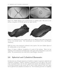
2.6 Spherical and Cylindrical Harmonics

2.6. SPHERICAL AND CYLINDRICAL HARMONICS 49Pierre-Simon Laplace really was French, having been born in Normandyin 1749. Laplace’s mathematical talents were recognized earlyand he moved to Paris when he was 19 to further his studies. Laplacepresented his first paper to the Académie des Sciences in Paris whenhe was 21 years old. He went on to make profound advances in differentialequations and celestial mechanics. Laplace survived thereign of terror and was one of the first professors at the new Ecole Normale in Paris.Laplace propounded the nebular hypothesis for the origin of the solar system in hisExposition du systeme du monde. He also advanced the radical proposal that therecould exist stars so massive that light could not escape them–we call these black holesnow And Traité du Mécanique Céleste is still print and widely read. Laplace alsomade fundamental contributions to mathematics, but I will mention only his bookThéorie Analytique des Probabilités. He died on the third of March 1827 in Paris.When solving boundary value problems for differential equations like Laplace’s equation,it is extremely handy if the boundary on which you want to specify the boundary conditionscan be represented by holding one of the coordinates constant. For instance, inCartesian coordinates the surface of the unit cube can be represented by:z = ±1 for − 1 ≤ x ≤ 1 and − 1 ≤ y ≤ 1y = ±1 for − 1 ≤ z ≤ 1 and − 1 ≤ x ≤ 1x = ±1 for − 1 ≤ z ≤ 1 and − 1 ≤ y ≤ 1On the other hand, if we tried to use Cartesian coordinates to solve a boundary valueproblem on a spherical domain, we couldn’t represent this as a fixed value of any of thecoordinates. Obviously this would be much simpler if we used spherical coordinates, sincethen we could specify boundary conditions on, for example, the surface r = constant.The disadvantage to using coordinate systems other than Cartesian is that the differentialoperators are more complicated. To derive an expression for the Laplacian in sphericalcoordinates we have to change variables according to: x = r cos φ sin θ, y = r sin φ sin θ,z = r cos θ. The angle θ runs from 0 to π, while the angle φ runs from 0 to 2π.Here is the result, the Laplacian in spherical coordinates:∇ 2 ψ(x y z) = 1 ∂r 2 ∂ψ +r 2 ∂r ∂r1r 2 sin θ∂sin θ ∂ψ +∂θ ∂θ1 ∂ 2 ψr 2 sin 2 (2.6.3)θ ∂φ 2

54 CHAPTER 2 WAVES AND MODES IN ONE AND TWO SPATIAL DIMENSIONSare defined as:The first few spherical harmonics are:Y m (θ φ) = 2 + 1 ( − m)4π ( + m) P m(θ φ)e imφ . (2.6.29)1Y 00 (θ φ) =(2.6.30)4π3Y 10 (θ φ) = cos θ (2.6.31)4π3Y 1±1 (θ φ) = ∓8π sin θe±iφ (2.6.32)5Y 20 (θ φ) =16π (2 cos2 θ − sin 2 θ) (2.6.33)15Y 2±1 (θ φ) = ∓8π cos θ sin θe±iφ (2.6.34)15Y 2±2 (θ φ) =32π sin2 θe ±2iφ (2.6.35)2.6.2 Properties of Spherical Harmonics and LegendrePolynomialsThe Legendre polynomials and the spherical harmonics satisfy the following “orthogonality”relations. We will see shortly that these properties are the analogs for functionsof the usual orthogonality relations you already know for vectors. 2π π004π −1−1 −1−1P (x)P (x)dx =P m(x)P m (x)dx =Y m (θ φ)Ȳ m(θ φ)dΩ =22 + 1 δ (2.6.36)2 ( + m)2 + 1 ( − m) δ (2.6.37)Y m (θ φ)Ȳ m (θ φ) sin θdθdφ = δ δ mm (2.6.38)

2.6. SPHERICAL AND CYLINDRICAL HARMONICS 55where the over-bar denotes complex conjugation and Ω represents solid angle: dΩ ≡sin θdθdφ. Using 4π as the limit of integration is symbolic of the fact that if you integratedΩ over the sphere (θ going from 0 to π and φ going from 0 to 2π) you get 4π. Noticethat the second relation is slightly different than the others; it says that for any givenvalue of m, the polynomials P m and P m are orthogonal.There is also the following “parity” property:Y m (π − θ φ + π) = (−1) Y m (θ φ). (2.6.39)orthogonal function expansionsThe functions P (x) have a very special property. They are complete in the set of functionson [−1 1]. This means that any (reasonable) function defined on [−1 1] can berepresented as a superposition of the Legendre polynomials:∞f(x) = A P (x). (2.6.40)=0To compute the coefficients of this expansion we use the orthogonality relation exactlyas you would with an ordinary vector. For example, suppose you want to know the x−component of a vector T. All you have to do is take the inner product of T with ˆx. Thisis becauseT = T xˆx + T y ŷ + T z ẑsoˆx · T = T xˆx · ˆx + T yˆx · ŷ + T zˆx · ẑ = T xsince ˆx · ẑ = ˆx · ŷ = 0 and ˆx · ˆx = 1. When you take the inner product of two vectorsyou sum the product of their components. The analog of this for functions is to sum theproduct of the values of the function at each point in their domains. Since the variablesare continuous, we use an integration instead of a summation. So the “dot” or innerproduct of two functions f(x) and g(x) defined on [−1 1] is:(f g) = 1−1f(x)g(x)dx. (2.6.41)So, to find the expansion coefficients of a function f(x) we take the inner product of fwith each of the Legendre “basis vectors” P (x): 1∞ 1∞f(x)P (x)dx = A P (x)P (x)dx =−1=0−1=0So, the -th coefficient of the expansion of a function f(x) isA = 2 + 12 1−1A 22 + 1 δ =2A 2 + 1 . (2.6.42)f(x)P (x)dx (2.6.43)

56 CHAPTER 2 WAVES AND MODES IN ONE AND TWO SPATIAL DIMENSIONSSimilarly, we can expand any function defined on the surface of the unit sphere in termsof the Y m (θ φ):∞ ψ(θ φ) = A m Y m (θ φ) (2.6.44)with expansion coefficientsA m ==0 m=−4πψ(θ φ)Ȳm(θ φ)dΩ. (2.6.45)For example, what is the expansion in spherical harmonics of 1? Only the = 0 m = 0spherical harmonic is constant, so1 = √ 4πY 00 .In other words, A m = √ 4πδ 00 .What is a field?The term “field” is used to refer to any function of space. This could be a scalarfunction or it could be a vector or even tensor function. Examples of scalar fieldsinclude: temperature, acoustic pressure and mass density. Examples of vector fieldsinclude the electric and magnetic fields, gravity, elastic displacement. Examples oftensor fields include the stress and strain inside continuous bodies.2.7 Exercises1. Apply separation of variables to Laplace’s equation in cylindrical coordinates:∇ 2 ψ(r θ z) = 1 r∂r ∂ψ + 1 ∂ 2 ψ∂r ∂r r 2 ∂θ + ∂2 ψ2 ∂z = 0. 2answer: We make the, by now, standard assumption that we can write the solutionin the form ψ(r θ z) = R(r)Q(θ)Z(z). Plugging this into Laplace’s equation anddividing by RQZ we have:1 dr dR + 1 d 2 QRr dr dr r 2 Q dθ + 1 d 2 Z2 Z dz . (2.7.1)2At this point we have a choice as to the order of the solution. We could first isolatethe z equation or we could isolate the θ equation. Also, in choosing the sign of theseparation constant, we are in effect choosing whether we want an exponentiallydecaying solution or a sinusoidal one. I suggest isolating the θ equation first since