Chapter 8 Vector Spaces in Quantum Mechanics

More documents

Recommendations

Info

Chapter 8 Vector Spaces in Quantum Mechanics 104The probability amplitude 〈x|ψ〉 appearing in Eq. (8.80) are functions of the continuousvariable x, and is often written 〈x|ψ〉 = ψ(x), which we identify as the wave function ofthe particle. If we now consider the inner productor〈x ′ |ψ〉 =ψ(x ′ ) =∫ +∞−∞∫ +∞−∞〈x ′ |x〉〈x|ψ〉dx (8.82)〈x ′ |x〉ψ(x)dx (8.83)we now see that we have an interesting difficulty. We know that 〈x ′ |x〉 = 0 if x ′ x, soif 〈x|x〉 is assigned a finite value, the integral on the right hand side will vanish, so thatψ(x) = 0 for all x!! But if ψ(x) is to be a non-trivial quantity, i.e. if it is not to be zero forall x, then it cannot be the case that 〈x|x〉 is finite. In other words, 〈x ′ |x〉 must be infinitefor x = x ′ in some sense in order to guarantee a non-zero integral. The way in which thiscan be done involves introducing a new ‘function’, the Dirac delta function, which hassome rather unusual properties.What we are after is a ‘function’ δ(x − x 0 ) with the property thatf (x 0 ) =for all (reasonable) functions f (x).∫ +∞−∞δ(x − x 0 ) f (x)dx (8.84)So what is δ(x − x 0 )? Perhaps the simplest way to get at what this function looks like isto examine beforehand a sequence of functions defined byD(x, ɛ) = ɛ −1 −ɛ/2 < x < ɛ/2= 0 x < −ɛ/2, x > ɛ/2. (8.85)
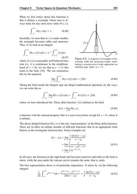
Chapter 8 Vector Spaces in Quantum Mechanics 105What we first notice about this function isthat it defines a rectangle whose area is alwaysunity for any (non-zero) value of ɛ, i.e.∫ +∞−∞D(x, ɛ)dx = 1. (8.86)Secondly, we note that as ɛ is made smaller,the rectangle becomes taller and narrower.Thus, if we look at an integralf (x)∫ +∞−∞∫ ɛ/2D(x, ɛ) f (x)dx = ɛ −1 f (x)dx−ɛ/2(8.87)where f (x) is a reasonably well behaved function(i.e. it is continuous in the neighbourhoodof x = 0), we see that as ɛ → 0, thistends to the limit f (0). We can summarizethis by the equationFigure 8.6: A sequence of rectangles of decreasingwidth but increasing height, maintaininga constant area of unity approaches aninfinitely high ‘spike’ at x = 0..∫ +∞lim D(x, ɛ) f (x)dx = f (0). (8.88)ɛ→0−∞Taking the limit inside the integral sign (an illegal mathematical operation, by the way),we can write this as∫ +∞−∞lim D(x, ɛ) f (x)dx =ɛ→0∫ +∞−∞δ(x) f (x) = f (0) (8.89)where we have introduced the ‘Dirac delta function’ δ(x) defined as the limitδ(x) = limɛ→0D(x, ɛ), (8.90)a function with the unusual property that it is zero everywhere except for x = 0, where itis infinite.The above defined function D(x, ɛ) is but one ‘representation’ of the Dirac delta function.There are in effect an infinite number of different functions that in an appropriate limitbehave as the rectangular function here. Some examples are1 sin L(x − x 0 )δ(x − x 0 ) = limL→∞ π x − x 01 ɛ= lim(8.91)ɛ→0 π (x − x 0 ) 2 + ɛ 21= limλ→∞ 2 λe−λ|x−x 0| .In all cases, the function on the right hand side becomes narrower and taller as the limit istaken, while the area under the various curves remains the same, that is, unity.The first representation above is of particular importance. It arises by via the followingintegral:∫1 +Le ik(x−x0) dk = eiL(x−x0) − e iL(x−x 0)= 1 sin L(x − x 0 )(8.92)2π −L2πi(x − x 0 ) π x − x 0x
Page 1 and 2: Chapter 8Vector Spaces in Quantum M
Page 3 and 4: Chapter 8 Vector Spaces in Quantum
Page 27: Chapter 8 Vector Spaces in Quantum
Page 33: Chapter 8 Vector Spaces in Quantum

Chapter 8 Vector Spaces in Quantum Mechanics

You also want an ePaper? Increase the reach of your titles

Delete template?

Save as template?