MS Thesis R. Hager - Hawaii National Marine Renewable Energy ...
MS Thesis R. Hager - Hawaii National Marine Renewable Energy ... MS Thesis R. Hager - Hawaii National Marine Renewable Energy ...
5. Highlight Diffraction + Froude-Krylov to view results. Data under Graph Datamay be highlighted and copied into Microsoft Excel.Figure 4. 25 Exciation Force ResultsIn the Workspace the cells should have a complete status icon, as seen in Figure 4.26.Figure 4. 26 Analysis System CompleteAs seen in Figure 4.25, the forces are calculated per unit wave amplitude since the excitationforce is a transfer function. To calculate the force for a particular wave height, simply72
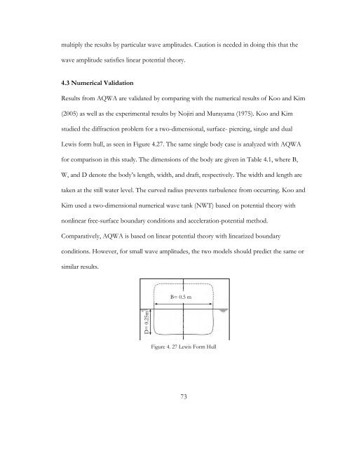
multiply the results by particular wave amplitudes. Caution is needed in doing this that thewave amplitude satisfies linear potential theory.4.3 Numerical ValidationResults from AQWA are validated by comparing with the numerical results of Koo and Kim(2005) as well as the experimental results by Nojiri and Murayama (1975). Koo and Kimstudied the diffraction problem for a two-dimensional, surface- piercing, single and dualLewis form hull, as seen in Figure 4.27. The same single body case is analyzed with AQWAfor comparison in this study. The dimensions of the body are given in Table 4.1, where B,W, and D denote the body’s length, width, and draft, respectively. The width and length aretaken at the still water level. The curved radius prevents turbulence from occurring. Koo andKim used a two-dimensional numerical wave tank (NWT) based on potential theory withnonlinear free-surface boundary conditions and acceleration-potential method.Comparatively, AQWA is based on linear potential theory with linearized boundaryconditions. However, for small wave amplitudes, the two models should predict the same orsimilar results.B= 0.5 mD= 0.25mFigure 4. 27 Lewis Form Hull73
- Page 21 and 22: CHAPTER 2. WAVE ENERGY CONVERSION D
- Page 23 and 24: 2.3 OrientationOrientation is defin
- Page 25 and 26: Figure 2.4 Oscillating Water Column
- Page 27 and 28: 2.5 Reference PointMeans of reactio
- Page 29 and 30: Linear GeneratorTurbineRotary Gener
- Page 31 and 32: Table 2. 1 WEC ClassificationsDevic
- Page 33 and 34: 33P.T.O.MooringReferencePointOperat
- Page 35 and 36: CHAPTER 3. THEORY AND GOVERNING EQU
- Page 37 and 38: F(x,z,t) z 0DFDtFt u F 0 0 (4
- Page 39 and 40: in ni(13)on S for i=1, 3in( r n)i3
- Page 41 and 42: I iAg e ekz i( kx t)(30)cosh( k(z
- Page 44 and 45: where ijkis the permutation symbol.
- Page 46 and 47: Mw k ieitS( D I) ijkrinjdS(46)3.3.3
- Page 48 and 49: Due to Kirchhoff decomposition, rec
- Page 50 and 51: TE KE PE 20L Asin(kx) 1 2(61)dV d
- Page 52 and 53: P I Iw dS (70)tnSIf the column
- Page 54 and 55: 221 2P gA C(77)max g2 3.8 Maximum
- Page 56 and 57: 4.2 AQWA Modeling ProcedureThe user
- Page 58 and 59: : Local data has changed, and the c
- Page 60 and 61: Figure 4. 5 Drawing in Design Modul
- Page 62 and 63: 12. Delete all lines inside the cur
- Page 64 and 65: 22. Edit the details of the slice u
- Page 66 and 67: Figure 4. 15 Details of the Part7.
- Page 68 and 69: Figure 4. 17 Details of the Mesh4.2
- Page 70 and 71: Figure 4. 21 Detials of the Wave Di
- Page 74 and 75: Table 4.1 Body Dimensions for Numer
- Page 76 and 77: concavity from concave down to conc
- Page 78 and 79: Figure 4. 29 Maximum Power Absorpti
- Page 80 and 81: Table 4. 3 Numerical ResultsBodyNo.
- Page 82 and 83: BodyNo.Bodyλ atT=2.1λ atT=1.0λ a
- Page 84 and 85: WAVEFigure 5. 1 Body Faces Wave Mak
- Page 86 and 87: The body connects to the aluminum p
- Page 88 and 89: also allowed for flexibility in cre
- Page 90 and 91: AB1 23 4 5 6 7CD8 9 10 11EFigure 5.
- Page 92 and 93: and minimum voltage range of the DA
- Page 94 and 95: Figure 5. 11 Deleting a Step from L
- Page 96 and 97: Figure 5. 14 Recording Options, Sig
- Page 98 and 99: Figure 5. 17 Right-mouse Click on t
- Page 100 and 101: Zero-OffsetThe Zero-Offset step rem
- Page 102 and 103: Figure 5. 24 Filter Step Set-up, Co
- Page 104 and 105: 5.6 Data ProcessingFigure 5. 26 Wav
- Page 106 and 107: 5.8 Experimental DiscussionAs menti
- Page 108 and 109: 5.8.3 Suggestions for Future Resear
- Page 110 and 111: 110ikxxRekddzkgkn )cosh())(cosh(,
- Page 112 and 113: Proof M ij and B ij are Symmetric T
- Page 114 and 115: BIBILIOGRAPHYANSYS. (n.d.). ANSYS A
- Page 116: Trust, C. (2011). Capital, Operatin
multiply the results by particular wave amplitudes. Caution is needed in doing this that thewave amplitude satisfies linear potential theory.4.3 Numerical ValidationResults from AQWA are validated by comparing with the numerical results of Koo and Kim(2005) as well as the experimental results by Nojiri and Murayama (1975). Koo and Kimstudied the diffraction problem for a two-dimensional, surface- piercing, single and dualLewis form hull, as seen in Figure 4.27. The same single body case is analyzed with AQWAfor comparison in this study. The dimensions of the body are given in Table 4.1, where B,W, and D denote the body’s length, width, and draft, respectively. The width and length aretaken at the still water level. The curved radius prevents turbulence from occurring. Koo andKim used a two-dimensional numerical wave tank (NWT) based on potential theory withnonlinear free-surface boundary conditions and acceleration-potential method.Comparatively, AQWA is based on linear potential theory with linearized boundaryconditions. However, for small wave amplitudes, the two models should predict the same orsimilar results.B= 0.5 mD= 0.25mFigure 4. 27 Lewis Form Hull73


