Delay Analysis of VLSI Interconnections Using the Di usion Equation ...

Delay Analysis of VLSI InterconnectionsUsing the Diusion Equation Model Andrew B. Kahng and Sudhakar MudduUCLA Computer Science Department, Los Angeles, CA 90024-1596AbstractThe traditional analysis of signal delay in a transmissionline begins with a lossless LC representation,which yields a wave equation governing the system response;2-port parameters are typically derived andthe solution is obtained in the transform domain. Inthis paper, we begin with a distributed RC line modelof the interconnect and analytically solve the resultingdiusion equation for the voltage response. A newclosed form expression for voltage response is obtainedby incorporating appropriate boundary conditions forinterconnect delay analysis. Calculations of 50% and90% delay times for various cases of interest (e.g.,open-ended RC line) give substantially dierent estimatesfrom those commonly cited in the literature,thus suggesting revised delay estimation methodologiesand intuitions for the design of VLSI interconnects.The discussion furthermore provides a unifyingtreatment of the past three decades of RC interconnectdelay analyses.1 OverviewDelay analysis of VLSI interconnections is a key elementin timing verication, gate-level simulation andperformance-driven layout design. The standard approachtomodelinginterconnect delay has been basedon a simple lossless LC model which considers onlyinductances (L) and capacitances (C). For this losslessmodel, the relationship between v and i gives riseto a second-order partial dierential equation of theform [9]:@ 2 v@x 2= LC @2 v@t 2 (1)and the solution to this wave equation is of the formv(x) =A 1 e x + A 2 e ,x (2) This work was supported byNSFYoung InvestigatorAwardMIP-9257982. Part of the work of S. Muddu was done duringthe course of a Summer 1993 internship at Intel Corporation.where propagation constant p |! lc (l and c arethe inductance and capacitance per unit length, and! is the wave frequency).One easily extends this model to lossy (RLC) interconnectsby incorporating a series resistance. Thesame equations obtained for the lossless model canbe used, with Z L = R + |!L = |![ R + L]; i.e.,|!Z L = |!L 0 where L 0 = R + L is the new inductance|!value. Similarly, one may incorporate a conductanceG via Z C = G + |!C = |![ G + |! C]; i.e., Z C = |!C 0where C 0 = G + C is the new capacitance. The same|!solution derived for the lossless model can incorporatethe new L 0 and C 0 values to capture the attenuationfactor in lossy lines.Using the solution (2) to the wave equation, andthe characteristic impedance of the line, one may treatthe interconnect line as a 2-port and obtain equationsfor voltage and current at the terminal side of the 2-port in terms of voltage and current at the source side.This yields the 2-port matrix parameters, e.g., ABCDparameters. To obtain the transient time-domain responseof an interconnect line, the standard approachhas been to calculate the response in the transform domainusing 2-port parameters, and then apply inversetransforms to obtain the response in the time domain.We call this the LC analysis, or wave equation, approach.Since it may be complicated to apply the inversetransforms, various approximations are typicallymade which simplify the resulting expressions for thetime-domain response.For the well-studied case of an RC transmissionline, the traditional LC analysis is extended to anRLC analysis after which L is set to zero. But bycontrast, if we initially model the interconnect as apure distributed RC line, we obtain a diusion equation(or heat equation) from which the solution forthe transient response, depending on boundary conditions,can be calculated analytically. This RC-baseddelay analysis approach, and its implications, are thesubject of the present paper.Our motivation for adopting the RC-based delayanalysis is as follows. For previous generation interconnects,such as for PCB, the resistance per unitlength (r) is considerably smaller than the inductiveimpedance (!l), i.e., r !l, so that the conventionalLC-based analysis seems reasonable. However, withsmall feature sizes of thin-lm and IC interconnects,we now nd that r !l up to frequencies of O(1)

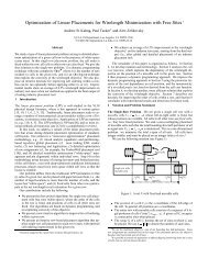
v 2 (t) V 04 p RC[1 , e ,2:467 tRC ] (t RC) (9)Sakurai [20] uses a similar 2-port model and obtainsthe voltage response asv 2 (t) =V 0 (1 , 1:273e ,2:467 tRC+0:424e,22:206 tRC )(10)These works, particularly [25], have had great inuenceon the literature. For example, Saraswat and Mohammadi[21] use the results of [15, 25] to obtain theirrise time estimates. Bakoglu and Meindl [4] also citeWilnai's derivation, and write: \Under step-voltageexcitation, the times (T ) required for the output voltageof distributed and lumped RC networks to risefrom 0 to 90 percent of their nal values are 1:0RCand 2:3RC, respectively." ([4], p. 904). The authorsof [4] go on to state a \very good approximation fordelay":T = 1:0R int C int +2:3(R tr C int + R tr C L + R int C L ) (2:3R tr + R int )C int (11)(R int and C int are respectively the interconnect resistanceand capacitance, R tr is the output resistance ofthe driving transistor and C L is the load capacitance).This last expression (11) has been frequently invokedin the literature (see [1], [22] orthebook[3]).Interestingly, the voltage response for a step inputusing the 2-port model has been rederived manytimesin the literature. For example, Antinone and Brown[2] express cosh( p sRC) as an innite product seriesand then consider only the rst three terms of theproduct expansion. This is not a good approximationbecause the coecients of s and s 2 are not exact, anddepend heavily on the number of terms used in theproduct expansion. Mey [17] noted the crudeness ofthis approximation and proposed an innite partialfraction expansion, thus obtaining the same solutionas Sakurai. Ghausi and Kelly [11] are yet anothergroup who earlier published the identical analysis.The common feature of all these works is that theyuse the 2-port transfer matrix of the distributed RCline to obtain their respective time-domain estimatesof the transient response. The 2-port parameters forthe distributed RC line are obtained from the solutionof the wave equation (2) for v and i (see, e.g., [9]). Butas we discuss in Section 3 below, voltage or current ina pure distributed RC line obeys a diusion equation.2.2.2 A Previous Time-Domain AnalysisFinally, a solution which uses time-domain analysis isthat of Kaufman and Garrett [15], who formulate adistributed RC model for interconnect and derive adiusion equation for voltage on the line. However,to obtain the transient response to a step input, [15]makes the simplifying assumption v(x; t) =f(x)g(t),namely, separability ofthevoltage response into separatefunctions of time and position; this leads to acomplicated and special-case solutionv 2 (t) =1, 4 1Xn=0(,1) n2n +1 e,((2n+1)=2)2 t=RC(12)Considering only the rst few terms of the series yieldsv 2 (t) (1 , 1:273e ,2:467 tRC +0:424e,22:206 tRC )(13)This expression is dierent from that of Wilnai orPeirson, but is identical 1 to that given by Sakurai(Equation 10). The book of Ghausi and Kelly [11]gives an analysis using the same separability assumption.These previous delay approximations are summarizedin Table 1 below.3 The Diusion Equation Analysis3.1 Obtaining the Diusion Equationfrom the Distributed RC Modeli(x,t) i(x+dx,t) r(x) dxv(x,t)xc(x) dxv(x+dx,t)x+dxc(x) dxr(x) dxFigure 2: Lumped approximation for x in adistributed RC line.The diusion equation for voltage in a distributedRC line can be derived from rst principles as follows(see [15]). Consider a lumped approximation for xof the line, as shown in Figure 2. By applying simplenodal equations at the nodes x and x +x, we obtain@v(x; t)i(x; t) = c(x)x + i(x +x; t)@tv(x; t) = r(x)xi(x +x; t)+v(x +x;t)where r(x) and c(x) are resistance and capacitanceper unit length. As x ! 0, and for constant r(x)and c(x), the above equations reduce to the diusionequationrc @v@t = @2 v@x : (14)2The solution of Equation (14) can be obtained byrestricting it to the set of solutions of the form v( x p t)p rcusing the substitution variable = x [14]. This is2tthe appropriate substitution for a parabolic equation.We obtainv() =C 1Z 0e , 22 d + C 2 (15)One can also obtain this solution directly from theheat kernel for the diusion equation [7]. This shouldbe contrasted with the solution of [15], which mustassume the separable form for v(x; t). Of course, thesolution we obtain will be highly dependent on theboundary conditions that apply; in particular, we areinterested in the well-studied case of the open-endeddistributed RC line.1In the taxonomythatwe present below, the result of Kaufmanand Garrett is characterized as \approximate" becausetheir method must assume the special form of the diusion equationsolution. On the other hand, Sakurai's result is \exact"with respect to the distributed RC 2-port analysis.

Method Accuracy/ Time-DomainRegimeVoltage ResponseSimple Approximate V 0 (1 , e , RC t)Lumped ModelWilnai's Small t 2V 0 (1 , erf(2-port ModelLarge tMattes'sExactqRC4t ))V 0 (1 , 1:366e ,2:5359 tRC +0:366e ,9:4641 tRC )P 2-port Model 1q2V 0 n=1 (,1)n,1 1 , erf( 2n,12qPeirson's Small t 2V 0 (1 , erf(RC4t ))2-port Model Large t V 0 1:273 p RC(1 , e ,2:467 tSakurai'sExact but2-port Model approximated V 0 (1 , 1:273e ,2:467 RCtto three termsKaufman's Heuristic derivationDiusion but approximated V 0 (1 , 1:273e ,2:467 RCtEquation Model to three termsAntinone/Brown's2-port modelApproximateV 0 (1 , 1:172e ,2:467 tRC+0:195e ,22:206 tRCOur Diusion Exact V 0 (1 , erf(Equation ModelRC )RC) t+0:424e ,22:206 tRC )+0:424e,22:206 tRC )qRC4t )), 0:023e ,61:685 tRC )Table 1: Voltage response of an open-ended distributed RC line under a step input excitation ofmagnitude V 0 . () Response calculated from the transfer function in [PB69].3.2 Boundary ConditionsFor the distributed RC line, we derive the twoboundary conditions necessary to solve Equation (15)as follows.Boundary Condition 1: At t = 0, the line is quietand v(x; t) = 0 for all x, i.e.,Therefore,C 1r2 + C 2 =0:C 2 = ,C 1r2(16)Note that this boundary condition applies to everynew wave that is born due to reection.Boundary Condition 2: The second boundarycondition is obtained from the structure of the inputapplied at the front end of the transmission line(x = 0) and in terms of the rise-time value, t rise . Noticethat the voltage at x = 0 depends on the sourceimpedance, Z S , and the characteristic impedance ofthe line, Z 0 , since this structure acts as a voltage divider.Therefore the voltage at the beginning of theline, i.e at x = 0, in the transform domain is given byV 1 (s) =(Z in) V 0Z in + Z S s(17)where Z in is the input impedance looking into the interconnectline.At a given rise-time (t = t rise ), the voltageV 1 (0;t rise ) at the front end of the transmission line canbe obtained from the time domain representation ofEquation (17). Let rise V 0 be this voltage at the risetime,i.e., V 1 (0;t rise )= rise V 0 , where 0 < rise 1.Substituting into Equation (15) and evaluating atx = , with tending to 0, we obtain rise V 0 = C 1Z p rc2t rise0e (, 2 2 ) d + C 2 (18)3.3 Solution of the Diusion EquationWe use (16) and (18) to solve forC 1 and C 2 :Z prcr2t rise rise V 0 = C 1 e (, x2 2 ) dx , C 12yieldsfrom whichC 1 = rise V 0 01[ R p rc2t rise0e , x2 2 dx , p 2 ]V () = rise V 0 [1 , erf( p2)] (19)

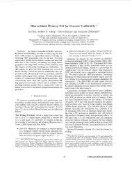
1where =[1,erf( 2p : rct)] riseTo achieve the case of an ideal step input, theboundary condition at x = 0 should be evaluatedfor t rise tending to zero and rise tending to 1, i.e.,we let t rise = " with " ! 0. Then, the error functionargument in the expression for will tend tozero, since and " both tend to zero with the numeratorof higher degree than the denominator, i.e.,lim rc!0;"!0 2p=0: Therefore, = 1 and the diusionequation solution reduces"toV () =V 0 [1 , erf( p2)]: (20)modied to consider the new delay values obtainedabove. We emphasize that our result does not implythat the previous LC-based approach is wrong.Rather, our work simply shows that solving the diusionequation for RC interconnects yields a very differentperspective ondelay calculations. A careful experimentalinvestigation is needed to determine therespective regimes for which these models are valid.Voltage1.11Open-Ended Distributed RC Line DelayPeirson’s ModelWilnai’s and Kaufman’s ModelsObserve that the same result is obtained when theinput corresponds to an ideal source, i.e., Z S = 0,V 1 (s) = V0 ,withvoltage at x = 0 constant for all tsand equal to V 0 . Inthiscase,V (0;t)=V 0 u(t) andusing this condition in Equation (15) yields0.90.80.70.60.5Lumped ModelDiffusion Equation ModelV 0 = C 1Z =xp rc2t =0from which C 2 = V 0 and0e , x22 dx + C 2V () =V 0 [1 , erf( p2)]: (21)This result is the same as Equation (20), as we expect.The same Equation (20) can also be obtained byusing the Boundary Condition 2 and another boundarycondition which captures the open end of the line[14]. We believe that the voltage on the line will betterobey Equation (20) near the source than near the load;ongoing experimental eorts are aimed at validatingthis belief. A comment is in order: the two boundaryconditions we use are discontinuous (at x =0,t = 0),but this discontinuity smooths immediately and thesolution is still valid.3.4 Threshold Delay Calculations UsingDiusion Equation ModelWe now proceed with delay calculations for a casethat has been of interest throughout the literature,namely, the open-ended distributed RC line with anideal source. Recall that with an ideal step input, = 1 in (19), the solution reduces to that given in(20). The equation for the voltage response for anideal source is obtained in Equation (21). Using errorfunction tables, we easily calculate the time for a signalapplied at the input of an interconnect to reach agiven threshold voltage at distance x (on the line) fromthe input terminal. For example, our diusion equationsolution implies 2:18R x C x for 63% delay time.One can see that the delay times for the diusionequation model are substantially dierent from thosecommonly employed in the literature, i.e., the Elmoredelay (for a single RC line) of t x (63%) = RxCx2. Thisdierence would certainly aect standard delay estimates:for example, minimum clock skew routing resultswhich use lumped models will be aected when0.40.30.20.1t/RC00 1 2 3 4 5Figure 3: Unit step response for lumped RCmodel and various distributed RC models. Notethat Wilnai's and Kaufman's models are notidentical: Kaufman's ( Sakurai's) model givesa non-monotone response. Also note that the responsein Peirson et al.'s model is dependent onthe RC constant; we have plotted the responsefor RC =1.4 Extensions of the Diusion EquationAnalysisWe close our development by extending the basicresult of Equation (20) in two ways: (i) introducingan analysis of reections, and (ii) incorporating nonzerotime of ight into the analysis.4.1 Analysis of ReectionsRecall that the total voltage on the line is given bythe summation of the incident wave and all reectedwave components. The reections are due to discontinuities,e.g., at the source (S) and load (L). In otherwords,~V Tot () =V I ()+1Xi=1~V Ri () (22)where V I () voltage corresponding to the incidentwave and ~ V Ri () voltage corresponding to the i threected wave. Neglecting the time of ight, at anytime the expressions for any individual ~ V Ri () will beof the same form as the incident voltage expressionV I (), but with dierent initial voltage. The solutionfor V I () isgiven by (19) in general, and by (20) for

an ideal step input. We use these expressions to calculatethe total voltage on the line for general sourceand load impedances. Note that since Z S and Z L arein general complex, we must treat V Tot () and V Ri ()as phasors V ~ Tot () and V ~ Ri () which are functions oftime (t), distance (x) and frequency (!). If V ~ Tot ()is a phasor, the delay calculations should compare themagnitude of total voltage (i.e., absolute value of thephasor, j V ~ Tot ()j) with the threshold value of interest.Luckily, the assumptions in typical cases of interest,while in some ways unrealistic, make the analysistractable and aord lower bounds for the delay estimates.In the general case, the reection coecients are, S = ZS,Z0Z S+Z 0the load yieldsand , L = ZL,Z0Z L+Z 0. The rst reection at~V R1 () =, L V I ();the second reection at the source yields~V R2 () =, S , L V I ();and in general the i th reection gives ~ V Ri () =2, i , 2iL S V I() for i even, with the case of i odd beinganalogous. Using~V Tot () = V I ()+1Xi=1~V Ri ()= V I ()[1 + , L +, S , L + :::+, i 2L , i 2S + :::]and separating odd and even terms of the summation,we obtain the general solution~V Tot () = rise ( 1+, L1 , , L , S)V 0 [1 , erf( p2)]The form of this expression, i.e., as a sum of errorfunction terms, is quite intuitive.Wemay again consider examples of source and loadimpedances which have received particular attentionthroughout the literature. 2Case 1: Finite-length, open-ended RC transmissionline with ideal source.With Z L = 1 (i.e., , L = 1), an ideal source(Z S =0,, S = ,1 and rise = 1) implies that allof the input voltage P appears at x = 0. Recalling that1~V Tot () =V I () + V ~ i=1 Ri (); we see that with re-ection coecients equal to +1 or ,1, all reectionswill cancel. Thus, the summation term in the equationdisappears and we obtain the same result as inEquation (21):~V Tot () = V I () =V 0 [1 , erf( p2)]2 Note that , L and , S will always have an implicit frequencydependence, and therefore ~ j V Tot ()j will also depend on thefrequency.Case 2: Finite-length, open-ended RC transmissionline with perfectly matched source.With Z L = 1 (i.e., , L = 1) and source impedanceZ S = Z 0 (i.e., , S = 0), there is only the single (initial)reection at the load. Thus,~V Tot () = V I ()+ ~ V R1 ()= 2[ rise V 0 (1 , erf( p2))]In practice, the open-ended approximation of an interconnectis often used since the input impedance ofMOS devices is typically high compared to the characteristicimpedance of the line.4.2 Non-Zero Time of FlightLast, we note that the derivation of Equation (22)neglected the time of ight, T fl , and used identical expressionsfor incident and reected waves. For a maximumon-chip interconnect of length approximately1cm, the time of ight will be around 0:1ns [6]. However,the length of a typical single interconnect segmentwill be much smaller (on the order of 0:01cm)and T fl will be on the order of picoseconds. Since delaysfor typical operating frequencies of O(1) GHz areof the order of 0:1ns [8], one may reasonably neglectT fl in delay calculations, as has usually the case in theliterature. Nevertheless, T fl becomes signicant withshorter rise or delay times, or with longer interconnects(e.g., for large die or MCM substrates). Here,we show that our analysis can extend to non-zero T fl .The key observation is that taking T fl into accountwill only increase our delay estimates, and these estimatesare already larger than those in the literature.To account for a non-zero time of ight, we simplyrecord an additional displacement ofT fl for each successivereection. The total voltage on the line afterthe i th reection is~V Tot (x; t) =V I (xrrc1X2t )+i=1~V Ri (xr rc2(t , iT fl ) )For example, if we consider non-zero T fl in Case 2of the previous subsection, the 90% delay time for aline of length h is obtained as follows.rrcr rcV I (h2t )+~ V R1 (h2(t , T fl ) )=0:9V 0which impliesrerf( h rc)+erf( h 2 t h 2rrct h , T fl) 1:1As expected, non-zero T fl will increase the 90% delaytime. The Case 2 analysis provides an upperbound on the voltage response, so the actual delaytime is lower-bounded by this equation. One couldsolve the equation through an iterative process, startingfromavaluethat is computed assuming T fl =0.For other cases, e.g., Case 1 above, T fl > 0 does notaect the previous analysis since there are no reections.

5 SummaryA survey of three decades of interconnect delayanalyses reveals that the analysis of signal delay ina transmission line is traditionally performed startingwith a lossless LC representation and a wave equationfor the system response; the solution is obtainedin the transform domain via 2-port parameters. Inthis paper, we begin with a distributed RC line modelof the interconnect, which yields a diusion equationfor the voltage response. We have given a new analyticsolution of this equation incorporating appropriateboundary conditions, and have obtained estimatesfor 50% and 90% delay times at arbitrary locations onthe interconnect line that dier substantially from thedelay estimates currently employed in the literature.Beyond its many implications for revised delayestimationmethodologies (e.g., for performance-driven routingtree construction, minimum-skew clock distribution,or buer placement), our time-domain solutionalso yields new intuitions regarding design objectivesfor VLSI interconnects. Our approach also handlesthe case of non-zero T fl .Our result does not imply that the previous LCbasedapproach is wrong, but rather shows that solvingthe diusion equation for RC interconnects canprovide a totally new perspective on delay calculations.Thus, we are also pursuing the central challengeof experimentally validating both our new model andprevious delay modelsinvarious technology regimes.AcknowledgmentsWe thank Professor Ernest S. Kuh of UC Berkeley,Dr. Heinz Mattes of Siemens, and Professor WayneWei-Ming Dai and Mr. Haifang Liao of UC Santa Cruzfor many helpful discussions and comprehensive commentson two early drafts of this work. Subsequentdiscussions with Prof. Russell Caisch of UCLA andDr. Steven Altschuler of Microsoft Corp. have alsobeen very helpful. Part of this work was performedduring a sabbatical visit to UC Berkeley; the hospitalityof Professor Ernest S. Kuh and his research groupis gratefully acknowledged.References[1] M. Afghahi and C. Svensson, \Performance of Synchronousand Asynchronous Schemes for VLSI Systems", IEEETrans. on Computers, July 1992, pp. 858-872.[2] R. J. Antinone and G. W. Brown, \The Modeling of ResistiveInterconnectsfor Integrated Circuits", IEEE J. Solid-State Circuits 18, April. 1983, pp. 200-203.[3] H. B. Bakoglu, Circuits, Interconnections and Packagingfor VLSI, Addison Wesley, 1990.[4] H. B. Bakoglu and J. D. Meindl, \Optimal InterconnectionCircuits for VLSI", IEEE Trans. on Electron Devices, May1985, pp. 903-909.[5] J. Crank, The Mathematics of Diusion, 2nd ed., Oxford,Clarendon Press, 1975, pp 11-17.[6] W. M. Dai, \Performance Driven Layout for Thin-FilmMultichip Modules", Intl. J. of High Speed Electronics,1991, pp. 287-317.[7] E. B. Davies, Heat Kernels and Spectral Theory, CambridgeUniv. Press, 1989.[8] A. Deutsch, G. V. Kopcsay, V. A. Ranieri, J. K. Cataldo, etal., \High Speed Signal Propagation on Lossy TransmissionLines", IBM J. Res. Dev. 34 (1990), pp. 601-615.[9] L. N. Dworsky, Modern Transmission Line Theory andApplications, Wiley, 1979.[10] W. C. Elmore, \The Transient ResponseofDampedLinearNetworks with Particular Regard to Wideband Ampli-ers", J. App. Physics 19, Jan. 1948, pp. 55-63.[11] M. S. Ghausi and J. J. Kelly, Introduction to Distributed-Parameter Networks: With Application to Integrated Circuits,Holt, Rinehart and Winston, 1968.[12] M. Healey, Tables of Laplace, Heaviside, Fourier, and ZTransforms, W. & R. Chambers Ltd., 1967.[13] C. C. Huang and L. L. Wu, \Signal Degradation ThroughModule Pins in VLSI Packaging", IBM J. Res. and Dev.31(4), July 1987, pp. 489-498.[14] A. B. Kahng and S. Muddu, \Analysis of VLSI InterconnectionsBased on the Diusion Equation Model", UCLACS Dept. TR-940011, 1994.[15] W. M. Kaufman and S. J. Garrett, \Tapered DistributedFilters", IRE Trans. on Circuit Theory, Dec. 1962, pp.329-336.[16] H. L. Mattes, \Behavior of a Single Transmission LineStimulated With a Step Function", manuscript, Aug. 1993.[17] D. D. Mey, \A Comment on `The Modeling of ResistiveInterconnects for Integrated Circuits' ", IEEE J. Solid-State Circuits, Aug. 1984, pp. 542-543.[18] R. C. Peirson and E. C. Bertnolli, \Time-Domain Analysisand Measurement Techniques for Distributed RCStructures. II. Impulse MeasurementTechniques", J. App.Physics, June 1990, pp. 118-122.[19] J. Rubinstein, P. Peneld and M. A. Horowitz, \SignalDelay inRCTree Networks", IEEE Trans. on CAD, July1983, pp. 202-211.[20] T. Sakurai, \Approximation of Wiring Delay inMOSFETLSI", IEEE J. Solid-State Circuits, Aug. 1983, pp. 418-426.[21] K. C. Saraswat and F. Mohammadi, \Eect of Scaling ofInterconnections on the Time Delay of VLSI Circuits",IEEE J. Solid State Circuits SC-17(2), April 1982, pp.275-280.[22] M. B. Small and D, J. Pearson, \On-chip Wiring for VLSI:Status and Directions", IBM J. Res. and Dev. 34(6), Nov.1990, pp. 858-867.[23] R. S. Tsay, \Exact Zero Skew", Proc. IEEE Intl. Conf. onComputer-Aided Design, 1991, pp. 336-339.[24] L. P.P.P. van Ginneken, \Buer Placement in DistributedRC-Tree Networks for Minimal Elmore Delay", Proc. IEEEIntl. Symp. on Circuits and Systems, 1990, pp. 865-868.[25] A. Wilnai, \Open-Ended RC Line Model Predicts MOS-FET IC Response", EDN, Dec. 15, 1971, pp. 53-54.