Here - Stuff

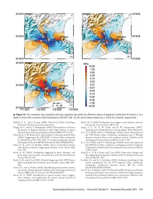
(A)(B)(C)▲▲Figure 13. The coseismic Δσ f caused by the two-segment slip model for different values of apparent coefficient of friction μ′ at adepth of 5 km with a receiver fault mechanism of 52°/61°/128°. A), B), and C) show results for μ′ of 0.0, 0.4, and 0.8, respectively.Dahlen, F. A., and J. Tromp (1998). Theoretical Global Seismology.Princeton, NJ: Princeton University Press.Dreger, D. S., and D. V. Helmberger (1993), Determination of SourceParameters at Regional Distances with Single Station or SparseNetwork Data, Journal of Geophysical Research 98, 8,107–8,125.Felzer, K. R., T. W. Becker, R. E. Abercrombie, G. Ekström, and J. R. Rice(2002), Triggering of the 1999 MW 7.1 Hector Mine earthquakeby aftershocks of the 1992 MW 7.3 Landers earthquake, Journalof Geophysical Research 107 B92190; doi:10.1029/2001JB000911.Felzer, K. R., and E. E. Brodsky (2006). Decay of aftershock densitywith distance indicates triggering by dynamic stress. Nature 441,735–738.Freed, A. M. (2004). Earthquake triggering by static, dynamic, andpostseismic stress transfer. Annual Review of Earth and PlanetarySciences 33, 335–367.Freed, A. M., and J. Lin (2001). Delayed triggering of the 1999 HectorMine earthquake by viscoelastic stress transfer. Nature 411, 180–183.Graves, R., and A. Pitarka (2010). Broadband ground motion simulationusing a hybrid approach. Bulletin of the Seismological Society ofAmerica 100, 2,095–2,123; doi: 10.1785/0120100057.Harris, R. A. (1998). Introduction to special section: Stress triggers,stress shadows, and implications for seismic hazard. Journal ofGeophysical Research 103, 24,347–24,358.Harris, R. A. (2000). Earthquake stress triggers, stress shadows, and seismichazard. Current Science 79 (9), 10.Jaeger, J. C., N. G. W. Cook, and R. W. Zimmerman (2007).Fundamentals of Rock Mechanics, fourth edition. Wiley-Blackwell.Ji, C., D. J. Wald, and D. V. Helmberger (2002a). Source description ofthe 1999 Hector Mine, California, earthquake, part I: Waveletdomain inversion theory and resolution analysis. Bulletin of theSeismological Society of America 92 (4), 1,192–1,207.Ji, C., D. J. Wald, and D. V. Helmberger (2002b). Source description ofthe 1999 Hector Mine, California, earthquake, part II: Complexityof slip history. Bulletin of the Seismological Society of America 92 (4),1,208–1,226.King, G. C. P., R. S. Stein, and J. Lin (1994). Static stress changes andthe triggering of earthquakes. Bulletin of the Seismological Society ofAmerica 84, 935–953.Lavallée, D., and R. J. Archuleta (2003). Stochastic modeling of slipspatial complexities for the 1979 Imperial Valley, California,earthquake. Geophysical Research Letters 30 (5), 1,245;doi:10.1029/2002GL015839.Liu, P., R. J. Archuleta, and S. H. Hartzell (2006). Prediction of broadbandground-motion time histories: Hybrid low/high frequencymethod with correlated random source parameters. Bulletin of theSeismological Society of America 96, 2,118–2,130.Seismological Research Letters Volume 82, Number 6 November/December 2011 813