Here - Stuff

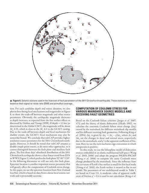
ERMJNUMAJOINUJHJ2CBIJMIDWJOWYHNBTPUB SSLB YULBNACB TATO YOJHKPSGUMOPATSWAKEKWAJJOHNKIPQIZDAVMANURABLXMASKKM LDMSBMKSMKUM IPMBTDF KOMPSIUGMKAPIPMGCOENMTNCCTTAO AKNRA QISWRABHNRAFIRARPPTFTAOEXMISMBWAWRKACOCOGIRLMORW KMBLBLDUMUNBBOOCASYVNDA SBAPAFQSPAMAWLCOPLCACRZFPMSAEFITRQAHOPE▲ ▲ Figure 6. Seismic stations used in the inversion of fault parameters of the 2011 Christchurch earthquake. These stations are chosenbased on their signal-to-noise ratio (SNR) and azimuthal coverage.tion. For each candidate depth and source duration, we alsoplot its best fitting focal mechanisms and magnitudes in Figure8, to show the trade-off between magnitude and other sourceparameters. Obviously, the earthquake magnitude decreasesas depth increases, as expected from the free surface effects asdiscussed by Dahlen and Tromp (1998). If depth = 12 km (asdetermined in the Global CMT), the magnitude will be aboutM w 6.15, which is close to the M w 6.1 in the GCMT catalog.Due to the trade-off between depth and focal mechanism forshallow events, the GCMT’s focal mechanism may also besomewhat biased. We conclude that teleCAP provides higherresolutionsource parameters for the 2011 Christchurch earthquake.However, it should be noted that teleCAP assumes adouble-couple point source, as do most other approaches, so itcannot distinguish between the fault plane and auxiliary faultplane. The first three days’ aftershock distribution of the 2011Christchurch earthquake shows a clear linear trend from EENto WWS (Figure 1), which prefers the fault plane 52°/61°/128°.In the following discussion we will use only this fault plane.Epicenter location is another important source parameter thatwill greatly affect the computation of Coulomb stress change.In this paper, we use the epicenter location from New ZealandGeoNet, which is based on data from a dense local seismic networkand is presumably accurate.COMPUTATION OF COULOMB STRESS FORVARIOUS MAINSHOCK SOURCE MODELS ANDRECEIVING FAULT GEOMETRIESBased on the Coulomb failure criterion (Jaeger et al. 2007,475) and the theory of elastic dislocation (Okada 1992), wecalculate the coseismic Coulomb failure stress change (Δσ f )caused by the mainshock for different mainshock slip modelsand for different receiving fault geometries. Following King etal. (1994), Δσ f is given by Δσ f = Δτ s – μ′Δσ n , where Δτ s andΔσ n are the changes in shear and normal stress, respectively,due to the mainshock, and μ′ is the apparent coefficient of friction.Here we use the rock mechanics sign convention in whichcompressive is positive.In this study, we use the lithosphere model of dislocationsources embedded in an elastic multilayered half space (Wanget al. 2003, 2006) and adopt the program PSGRN/PSCMP(Wang et al. 2006) to compute the static Coulomb stresschange produced by the mainshock. Since the influence fromthe curvature of Earth’s free surface is small for this local study(Xiong et al. 2010), the Earth surface is treated as flat in ourmodel. The parameters of our multilayered model in Table 1are based on Crust 2.0. A moderate value of apparent coefficientof friction μ′ = 0.4 is used in our calculation (King et al.806 Seismological Research Letters Volume 82, Number 6 November/December 2011